[

Levy-Nearest-Neighbors Bak-Sneppen Model

Abstract

We study a random neighbor version of the Bak-Sneppen model, where ”nearest neighbors” are chosen according to a probability distribution decaying as a power-law of the distance from the active site, $P(x)\sim|x-x_{ac}|^{-\omega}$. All the exponents characterizing the self-organized critical state of this model depend on the exponent $\omega$. As $\omega\to 1$ we recover the usual random nearest neighbor version of the model. The pattern of results obtained for a range of values of $\omega$ is also compatible with the results of simulations of the original BS model in high dimensions. Moreover, our results suggest a critical dimension $d_{c}=6$ for the Bak-Sneppen model, in contrast with previous claims.

]

Since its introduction, the Bak-Sneppen (BS) model [1] has had much success as perhaps the simplest and yet non-trivial self-organized critical (SOC) extremal model. Understanding its behavior is therefore very important to get an insight in the behavior of other SOC extremal models [2].

The BS model is easily defined: To each site $i$ on a hypercubic lattice in $d$ dimensions is assigned a random variable $f_{i}$ taken from a probability distribution $p(f)$, say, uniform in $[0,1]$. Then at each time-step the site $i$ with the smallest $f_{i}$ is chosen (it is called the active site), and its variable and the variables of its $2d$ nearest-neighbors are updated taking them from $p(f)$. As a result of this dynamics, the system organizes in a stationary state where almost all the variables $f_{i}$ are above a threshold $f_{c}$. Moreover, in this state, the dynamics of the model has self-similar features: each update of the minimum variable triggers a local avalanche of updates; the time durations of the avalanches obey a power-law distributions characterized by an exponent $\tau$. The number of sites touched by an avalanche of duration $t$ grows like $t^{\mu}$. Also the first return times (defined as the times between two successive returns of the activity to the same site) and the all return times (the times between the first passage of the activity on a site and any successive return to the same site) are power-law distributed, with exponents $\tau_{f}$ and $\tau_{a}$ respectively.

Not all of the above exponents are independent. Indeed it is possible to show, from renewal theory, that $\tau_{a}+\tau_{f}=2$ if $\tau_{a}<1$, $\tau_{a}=\tau_{f}$ if $\tau_{a}>1$ [3]. Recently, a non trivial relation between $\tau$ and $\mu$ has been unveiled in [4, 5] exploiting the hierarchical structure of the update avalanches (each avalanche is made up of smaller avalanches, and so on down to the microscopic scale). Both relations are satisfied for $d=1$ with $\tau\sim 1.07$ and $\mu\sim 0.42$, $\tau_{a}\sim 0.42$ and $\tau_{f}\sim 1.58$ [1, 2].

The only known exactly solved version of the BS model is the Random Nearest-Neighbor (RNN) model: there ”nearest neighbors” are chosen at random over the lattice[6]. As a result geometric correlations typical of low dimensions are lost, and the RNN can be considered as a Mean Field version of the BS model. The exponents of the RNN model are known to be $\tau=\tau_{a}=\tau_{f}=3/2$ and $\mu=1$[7]. In particular these exponents satisfy both $\tau_{a}=\tau_{f}$ and the relation between $\tau$ and $\mu$ proposed in [4]. In [5] this relation has been carefully studied, and it has been ”graphically” explicited (see Fig.1). The knowledge of the two exponent relations has given confidence in high-dimensional simulations [8] whose main result is that the upper critical dimension of the model is $d_{uc}=8$ (the upper critical dimension is the dimension above which the exponents should take the RNN values). This conclusion is at odds with previous claims, based on analogies of the BS model with directed percolation, that $d_{uc}$ should be $4$. A further result from [8] is the presence of two regimes as the dimension $d$ of the system increases: for $d\leq 3$ the model is recurrent ($\tau_{a}<1$; in random walk theory recurrence means that every site of the lattice is touched an infinite number of times with probability one), whereas for $d\geq 4$ the model is transient ($\tau_{a}>1$; transience means that there is a finite probability, smaller than $1$, that a site will be touched by the process), yet non trivial (i.e., different from the RNN model) as long as $d<8$. Actually, before [8], a further exponent relation was believed to hold, namely $\mu=\tau_{a}$. In [8] this relation is shown not to hold for $d>2$. Indeed, since $\mu\leq 1$ always and $\tau_{a}(RNN)=3/2$, it is straightforward to conclude that at least as soon as $\tau_{a}>1$, $\tau_{a}\neq\mu$. The dimensionality $d=3$, with $\tau_{a}<1$ and $\mu\neq\tau_{a}$, can be therefore considered as representative of a further regime within the recurrent one.

The BS model shows therefore an extremely rich behavior changing the dimensionality $d$ of the system. Yet, high-dimensional simulations are always susceptible of strong finite-size corrections, and the good convergence of the results is difficult to prove. In this Communication we propose a new way to interpolate between the $d=1$ and the RNN models: The ”nearest neighbors” of the active site $x_{ac}$ are chosen at random over the lattice, but with a probability that is a power-law decreasing function of the distance from it

$$P(x)\sim|x-x_{ac}|^{-\omega}\;\;.$$ (1)

As we will show, varying $\omega$ we find the same behavioral pattern as found in [8] varying $d$. We name this model the Levy-Random-Nearest-Neighbor model (LRNN; here the use of the word Levy is somehow an abuse since we use also $\omega>3$).

As a loose analogy, we recall that the same idea has been applied also to the $d=1$ Ising model with interactions decaying as (1), and indeed it has been found that, varying $\omega$ it is possible to go from the $d=1$ model to mean-field like results [9].

Simulations are performed over $1d$ lattices of up to $2^{19}$ sites, with growing sizes showing stability of the exponents.

In Fig.1 we show the $\tau$ avalanche exponents for different values of $\omega$ plotted against the corresponding values of $\mu$. All the $\mu/\tau$ pairs nicely satisfy the exponent relation between the two exponents obtained in [8]. This is a first important check of the consistency of our simulations and of the exponent relation.

In Fig.2 we plot the $\tau_{a}$, $\tau_{f}$ and $\mu$ exponents for different values of $\omega$ from $\omega=3$ to $\omega=1^{+}$ (this extreme value is not shown since simulations become extremely difficult due to the non normalizability of the distribution if $\omega=1$). Many important aspects of the model can be discussed looking at Fig.2. We find that the exponent relation between $\tau_{a}$ and $\tau_{f}$ is satisfied both when $\tau_{a}<1$ and when $\tau_{a}>1$. Therefore this result and Fig.1 confirm the validity of the two already known exponent relations. Moreover, we see that the exponents tend to their RNN values as $\omega\to 1$. This result should have been expected. Indeed the probability distribution (1) is normalizable in the thermodynamic limit only as long as $\omega>1$; when $\omega<1$ then the normalization is ruled by the length of the lattice

$$\int_{1}^{L}x^{-\omega}\sim L^{1-\omega}$$ (2)

that diverges in the limit of infinite lattice size $L$. Therefore the distribution $P(x)$, properly normalized, degenerates to $0$, just as in the RNN case, where the normalization is $1/L$ (case $\omega=0$).

The opposite case, $\omega\to\infty$, is also intriguing. Indeed we could naively expect the $d=1$ limit to be recovered when $\omega\geq 3$. In that case the average distance of the ”neighbors” and its variance are finite, just as for nearest neighbors. We would thus expect the $\omega>3$ case to belong to the same universality class as the original BS model, but this conclusion is not correct. In order to shed light on this problem, we also performed simulations taking the neighbors according to a distribution exponentially decreasing with respect to the distance from the active site $x_{ac}$. In this case, instead, we nicely recover the known $d=1$ exponents of the BS model. We conclude therefore that the presence of diverging moments of order higher than two drives the system out of its nearest neighbor fixed point. The latter holds instead whenever the distribution of the random neighbors has all its moments finite. This result, although non trivial, is not new in (annealed or quenched) disordered systems. For example, it has been shown that diverging moments of order higher than two in the disorder distribution can change the universality class of directed polymers in random environments, and of the related Kardar-Parisi-Zhang surface growth equation[10].

It is well known in classical random walk theory that random walks with a jump probability distribution with finite variance belong to the Gaussian universality class. Random walks with infinite higher moments have a microscopic structure that is different from a Gaussian one, mainly made of clusters of points seldom separated by long jumps. On larger and larger length scales, this cluster structure disappears, and the walks ”renormalize” to Gaussian ones. Yet, a main difference between a simple random walk and the BS model is the presence of memory effects. Indeed, any time a site is chosen (either as the active one or as one of its neighbors), any memory of its previous updates is lost. Therefore, the interaction between the geometric structure given by the choice of the neighbors according to $P(x)$ and the updates of the corresponding variables can give rise to non-trivial effects.

As already mentioned above, the geometrical fractal dimension $D_{f}$ of the avalanches is another quantity of interest. It is possible to relate $D_{f}$ to the other exponents of the model. Indeed, we recall that the fractal dimension relates the volume $N$ of the avalanche (that is, the number of sites touched by the avalanche) with the typical size $R$ of the avalanche, as $N\sim R^{D_{f}}$. On the other hand, $N$ scales with the duration of the avalanche as $N\sim t^{\mu}$. The relation between the typical size of the avalanche $R$, and its duration $t$ is given by $t\sim R^{z}$, $z$ being the dynamical exponent of the model. Then we find $D_{f}=z\mu$.

In principle, in order to determine $z$ it is possible to use the all return time distribution $P_{a}(t)$. At long times on a $d-$dimensional lattice of $N=L^{d}$ sites, $P_{a}(t)$ flattens. W e can write a scaling form for $P_{a}(t)$ as

$$P_{a}(t,L)=t^{-\tau_{a}}f\left(\frac{t}{L^{z}}\right)$$ (3)

with $f(x)\sim const$ when $x\to 0$ and $f(x)\sim x^{\tau_{a}}$ when $x\to\infty$. In this second case we find that $P_{a}(t,L)=L^{-d}$ (roughly speaking, as soon as every site of the lattice has been touched by an avalanche, they have all the same probability to be chosen), from which we have $z=d/\tau_{a}$.

Then we can write an expression for the fractal dimension

$$D_{f}=d\frac{\mu}{\tau_{a}}\;\;\;.$$ (4)

This expression holds for the high dimensional simulations of [8]: when avalanches are compact objects ($d=1,2$), $\mu=\tau_{a}$. Then, $\mu\neq\tau_{a}$ and avalanches become fractal objects. Indeed (4) approximates well the data given in [8] for $d=3$ ($\tau_{a}=0.92$, $\mu=0.85$, $D_{f}=2.6\simeq 3\mu/\tau_{a}=2.77...$) and for $d=4$ ($\tau_{a}=1.15$, $\mu=0.92$, $D_{f}=3.3\simeq 4\mu/\tau_{a}=3.2$). As a byproduct, we find that (4) suggests an upper critical dimension for the Bak-Sneppen model $d_{uc}=6$: indeed with $\mu=1$ and $\tau=3/2$ (the ”mean-field”, RNN, values of the exponents) we find $D_{f}(d=6)=4$, that is indeed the predicted avalanche fractal dimension in the RNN limit. $d_{uc}=6$ is at odds with what stated in [8], where $d_{uc}=8$ was suggested by numerical simulations, but also with [2] where $d_{uc}=4$ was claimed based on analogies with directed percolation.

Although (4) seems to hold in the high dimensional case, it does not fit the numerical results in the present LRNN approach. The reason is that, whereas in the high dimensional case there is a single relation between time and space, namely $t\sim L^{d/\tau_{a}}$, in the LRNN case there is a further relation, the usual Levy random walk law $t\sim R^{\omega-1}$. We measure the fractal dimension of avalanches using the distance between the rightmost and leftmost touched sites as a measure of $R$, and this corresponds to $z=\omega-1$. Indeed, as it can be seen from Fig.3, $D_{f}=\mu(\omega-1)$ approximates very well the measured fractal dimensions.

As noted above about the fractal dimension of high-dimensional avalanches, we observed that $\mu=\tau_{a}$ corresponds to compact avalanches. In the LRNN case we see from Fig.2 that indeed $\mu\neq\tau_{a}$ for $\omega<2$, even if the fractal dimension $D_{f}<1$ already for $\omega<3$. We can try to understand this result remembering that $D_{f}$ is related to the random walk exponent $z=\omega-1$: although $z$ is different from its Gaussian value $z=2$ as soon as $\omega<3$, a Levy random walk with $\omega>2$ is still compact, and so is the structure built by a choice of neighbors according to (1). Only when $\omega<2$ such a structure becomes genuinely fractal, and $\mu\neq\tau_{a}$.

The possibility to obtain the exponent $D_{f}$ from $\mu$ and $\tau_{a}$ in high dimensions, and from $\mu$ and $\omega$ in the LRNN version, suggests that indeed there are at most two independent exponents in the model, namely $\mu$ and $\tau_{a}$. The LRNN model suggests the presence of a further (although non trivial) exponent relation. Indeed, in Fig.4 we show the values of the $\tau_{a}$ exponent as a function of the corresponding $\mu$ exponent for different values of $\omega$ and for different dimensions. As it can be seen, the agreement is good, suggesting that the knowledge of $\mu$ (or of $\tau_{a}$) is sufficient to know all the other exponents through relations that, as for the $\mu/\tau$ one, could be highly non-trivial.

In conclusion, we have introduced a modification of the Bak-Sneppen model where the neighbors of the active site are chosen at random over the lattice with a probability that decreases like a power-law of the distance from the active site, with an exponent $\omega$. As a result we find that the characteristic exponents of the model interpolate between the $d=1$ limit ($\omega=\infty$) and the mean field (RNN) limit ($\omega\leq 1$). In particular, we verify that the known exponent relations hold for this model too. Moreover, we find and verify an exponent relation for the fractal dimension of the avalanches, $D_{f}=(\omega-1)\mu$. As a byproduct we obtain a relation between $D_{f}$ and $\mu$ and $\tau_{a}$ also in high dimensions, fitting well the present numerical results up to $d=4$[8], although it suggests an upper critical dimension $d_{uc}=6$ (and not $d_{uc}=4$ or $d_{uc}=8$ as previously believed). More accurate numerical simulations in high dimensions are therefore needed. The relevance of the results reported in this Communication is manifold: they can be looked at as an interesting modification of the Bak-Sneppen model, but their full importance emerges when compared to the high dimensional results of [8]. Indeed, they lead us to propose a new value of the upper critical dimension of the model, namely $d_{uc}=6$, and to conjecture the existence of a still undiscovered exponent relation between $\mu$ and $\tau_{a}$, reducing therefore the number of independent exponents to one in any dimension. This results show therefore that there is still some way to go before a full and satisfying understanding of the BS model is achieved.

The authors thank F. Slanina for useful discussions. R. Cafiero and P. De Los Rios aknowledge financial support under the European network project FMRXCT980183.

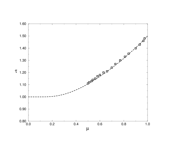
FIG. 1.: Avalanche exponent $\tau$ vs. $\mu$ for different Levy exponents $\omega$. The dashed line is the exact relation between the two exponents as from [5]. The data from the simulations and the exact relation are in excellent agreement. Error bars are comparable with the symbol dimensions.

FIG. 2.: Values of the different relevant exponents, $\mu$, $\tau_{a}$ and $\tau_{f}$, as a function of the Levy exponent $\omega$.

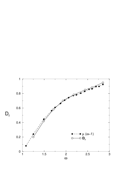
FIG. 3.: Avalanche fractal dimension $D_{f}$ for different values of $\omega$ (circles) and as from $D_{f}=(\omega-1)\mu$ (squares).

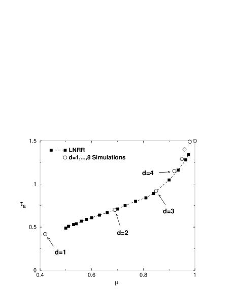
FIG. 4.: All return time exponent $\tau_{a}$ vs. $\mu$ for different values of $\omega$ (squares) and for different dimensions, from $d=1$ to $d=8$ (circles).

REFERENCES

- [1] P. Bak and K. Sneppen, Phys. Rev. Lett. 71, 4083 (1993).
- [2] M. Paczuski, S. Maslov, and P. Bak, Phys. Rev. E 53, 414 (1996).
- [3] M. Fisher, in Fundamental Problems in Statistical Mechanics VI, ed. E.G.D. Cohen, North-Holland (Amsterdam 1984).
- [4] S. Maslov, Phys. Rev. Lett. 77, 1182 (1996).
- [5] M. Marsili, P. De Los Rios and S. Maslov, Phys. Rev. Lett. 80, 1457 (1998).
- [6] H. Flyvbjerg, K. Sneppen, and P. Bak, Phys. Rev. Lett. 45, 4087 (1993).
- [7] J. de Boer, B. Derrida, H. Flyvbjerg, A.D. Jackson, and T. Wettig, Phys. Rev. Lett. 73, 906 (1994).
- [8] P. De Los Rios, M. Marsili and M. Vendruscolo, Phys. Rev. Lett. 80, 5746 (1998).
- [9] S.A. Cannas, Phys. Rev. B 52, 3034 (1995).
- [10] T. Halpin-Healy and Y.-C. Zhang, Phys. Reports 254, 216 (1995).