Kondo Effect in Systems with Spin Disorder

Abstract

We consider the role of static disorder in the spin sector of the one- and two-channel Kondo models. The distribution functions of the disorder-induced effective energy splitting between the two levels of the Kondo impurity are derived to the lowest order in the concentration of static scatterers. It is demonstrated that the distribution functions are strongly asymmetric, with the typical splitting being parametrically smaller than the average rms value. We employ the derived distribution function of splittings to study the temperature dependence of the low-temperature conductance of a sample containing an ensemble of two-channel Kondo impurities. The results are used to analyze the consistency of the two-channel Kondo interpretation of the zero-bias anomalies observed in Cu/(Si:N)/Cu nanoconstrictions.

I Introduction

The Kondo effect, that is the low-temperature screening of dynamical quantum defects in metals by band electrons, has been extensively studied during the past thirty years and is by now well understood (see, e.g., Refs. [1, 2]). The continuing interest in the problem is motivated chiefly by the search for novel realizations of the effect [3]. For example, local non-Fermi-liquid ground states have been predicted theoretically [4] for certain types of dynamical defects coupled to band electrons. The behavior of these impurities is sometimes invoked in efforts to understand the non-Fermi-liquid behavior of strongly correlated systems, such as heavy fermion materials and high-temperature superconductors [2].

One of the main difficulties encountered in the interpretation of experimental data from novel Kondo systems is the fact that defects with internal degrees of freedom very seldom represent the only type of disorder in the system. More often, a considerable number of random static defects affecting band electrons are also present. Scattering of electrons on this static disorder may alter the experimental signature of the Kondo effect [5, 6, 7, 8, 9, 10, 11, 12], sometimes masking genuine non-Fermi-liquid behavior, or, vice versa, possibly mimicking it in Fermi-liquid systems [13].

The Kondo effect requires that at least two internal states of the impurity be degenerate or, at least, that their energy difference be much smaller than the Kondo temperature $T_{K}$. Barring the cases of accidental degeneracy between the states of the dynamical impurity, degeneracy occurs as a consequence of a symmetry, e. g., invariance under time-reversal transformation in the case of the magnetic one-channel Kondo effect. Accordingly, the possible types of disorder can be separated into two classes, depending on whether disorder destroys the relevant symmetry of the Hamiltonian.

A typical example of the first class is a dilute magnetic alloy with a finite concentration of non-magnetic defects. Assuming that the charge state of the magnetic impurity does not change as a result of the interaction with conduction electrons (thus excluding the mixed-valence regime of the Anderson model), potential scattering on static disorder does not involve the degree of freedom of conduction electrons which is coupled to the magnetic impurity – their spin. The Hamiltonian remains invariant under time reversal, and the spin states of the impurity are degenerate even in the presence of disorder. The Kondo temperature $T_{K}$, on the other hand, is affected by potential scattering of electrons. The nature of the ground state in systems of this type has been studied in Refs. [6, 9, 10, 13].

Another example of such symmetry-preserving disorder is given by spin-orbit scattering [14, 15] in magnetic Kondo systems. The corresponding Hamiltonian is also invariant under time reversal, and Kramers’ theorem ensures that each orbital state of conduction electrons is doubly degenerate, so their coupling to magnetic impurities does not lift the degeneracy of impurity states.

An entirely different situation is encountered when scattering on static defects breaks the relevant symmetry. Kondo coupling between the band electrons and the dynamic defect then leads to symmetry-breaking contributions to the self-energy of the dynamic defect. The frequency-independent part of these contributions can be reinterpreted as an extra term in the bare Hamiltonian of the dynamic defect, and the difference between its eigenvalues (the energy difference between the “up” and “down” states of the defect) is an effective splitting $\Delta$. Being induced by random scattering, the splitting itself is a random quantity. This type of model was studied, for example, in Ref. [14], where the average splitting induced by broken time-reversal invariance due to the combined effect of random spin-orbit scattering and weak magnetic field was computed. A similar model has been encountered in the study of internal magnetic field distributions in spin glasses [16].

The present study of models of this type has been motivated in part by the discussion in Ref. [11] of different theoretical interpretations of zero-bias anomalies in Cu/Si:N/Cu nanoconstrictions [17]. The zero-bias anomalies first reported in Ref. [17] were observed in nanoconstrictions formed by etching a bowl-shaped cavity in an insulating $\mathrm{Si}_{3}\mathrm{N}_{4}$ substrate before covering both sides with vacuum-deposited Cu films. The anomalies are characterized by a $\sqrt{V}$ dip in conductance $G$ at small bias $V$, a corresponding $\sqrt{T}$ temperature dependence of conductance at $V=0$, and, more generally, a scaling function of the form $G\left(V,T\right)-G\left(0,T\right)=T^{1/2}\Gamma\left(V/T\right)$ where $\Gamma\left(x\gg 1\right)\propto x^{1/2}$. These features were interpreted in Refs. [17, 18] (see also Ref. [19] for additional experimental results and Ref. [20] for a comprehensive review) as consistent with the scaling properties at low temperatures of the two-channel Kondo model [4]. The observed absence of Zeeman splitting led to a conclusion [17] that a non-magnetic realization of the two-channel Kondo model of the type suggested by Vladár and Zawadowski [21] might be responsible for the observed anomaly.

The two-channel Kondo model, first proposed in Ref. [4] (see also Ref. [22] for an extensive review) to classify magnetic properties of rare earth materials, is characterized by doubling of the degrees of freedom of conduction electrons as compared to the usual one-channel case, while the dynamic impurity is still a “spin-up, spin-down” doublet. In other words, each orbital state of conduction electrons acquires, in addition to its spin, an extra label, “flavor”, which is silent in the sense that the scattering on the dynamic impurity conserves the flavor quantum number. Even so, the strongly correlated ground state of this model has been predicted to exhibit unusual and rather distinctive scaling properties, markedly different from the Fermi-liquid-like ground-state properties of ordinary Kondo impurities.

In the original model proposed in Ref. [4], the flavor degrees of freedom were constructed out of different angular momentum states of conduction electrons. Subsequently, it was proposed in a series of papers by Vladár and Zawadowski [21] that an effective two-channel Kondo model may emerge in an entirely different context, where the roles of orbital angular momentum and spin of conduction electrons are interchanged. The role of a dynamic impurity in such non-magnetic realizations of the Kondo effect is assumed to be played by a two-level system (TLS) – an atom or a group of atoms tunneling between two nearly degenerate states. If transitions between the two states of the TLS involve a transfer of charge, the transition amplitude becomes dependent on the density of conduction electrons via the Coulomb interaction [21]. The parity of electronic states with respect to the center of the spatially extended defect becomes the active degree of freedom – “pseudospin”. The physical spin assumes the role of the silent “flavor” degree of freedom, providing two independent channels (in the absence of spin scattering) for the screening of the dynamic impurity [4, 21]. Such TLS may be formed accidentally in a strained glassy material [23], or as a result of a Jahn-Teller effect [24], and TLS have also been conjectured to occur at interfaces [25]. Very recently, the non-Fermi-liquid properties of the ground state in this model have been invoked in the study of dephasing rate of conduction electrons in disordered metals [26].

The degeneracy between the two states of the TLS based on pseudospin symmetry is a crucial precondition for two-channel Kondo screening and the formation of the non-Fermi-liquid ground state. In practice this degeneracy is almost always expected to be lifted because the pseudospin, corresponding to parity about the center of the TLS, is not in general a conserved quantity, and, in particular, is not conserved by ordinary potential scattering. This feature of the orbital two-channel Kondo model has to be contrasted with magnetic Kondo models where the relevant symmetry is time-reversal invariance, which is broken only in special circumstances, e.g. by an applied magnetic field or magnetic disorder. Therefore, an analysis of the magnitude of disorder-induced splittings of two-level systems is essential in evaluating the consistency of the two-channel Kondo interpretation of the zero-bias anomalies of Refs. [17, 19].

Most of the previous theoretical work on this subject [11, 14] has been concentrated on computing the second moment of the random splittings. A calculation of $\left\langle\Delta^{2}\right\rangle$ induced by white-noise potential scattering was reported in Ref. [11]. It was argued there that even small amounts of disorder may lead to large splittings between the energy levels of the TLS, thus effectively stopping the Kondo screening at temperatures higher than $T_{K}$. However, the distributions of splittings tend to be very asymmetrical so that their moments are not representative of the typical values. Moreover, the knowledge of the full distribution function is necessary to understand how the splittings of an ensemble of defects may affect the scaling behavior of conductance.

It should be remarked that there is no direct evidence for the existence of TLS in the nanoconstrictions studied in the experiments of Refs. [17, 19]. It is precisely the match between the experimental scaling of conductance and that predicted theoretically for two-channel Kondo systems that is the main argument in favor of the two-channel Kondo interpretation of the data. The theoretical scaling functions used for this purpose in Refs. [17, 18] were derived under the assumption that no disorder other than the TLS themselves is present, and thus it is of considerable interest to understand how these scaling functions may be changed by realistic amounts of static disorder.

In this paper we study distribution functions of splittings for two models: (i) isotropic magnetic Kondo impurities in a spin glass environment, and (ii) atomic TLS in an environment of static defects inducing potential scattering. In both cases the disorder is modeled by an array of randomly located point scatterers. The magnetic model may be realized if a dilute solution of weakly coupled magnetic impurities undergoes Kondo screening in a spin-glass environment, formed, for example, by a more concentrated solution of more strongly coupled magnetic impurities. The result for the distribution of splittings in this case reproduces the distribution of internal fields in spin glasses derived earlier in Ref. [16]. We also analyze the effects of higher-order terms in the Kondo coupling which cannot be reduced to RKKY-type expressions. These terms are shown to lead to a finite renormalization of the small-$\Delta$ portion of the distribution functions, while their effect on the large-$\Delta$ tail is negligible. A similar analysis is performed for the distribution of splittings of atomic TLS. The magnitude of the splittings obtained here should be viewed as a lower bound, since only effects of electronic disorder are taken into account, i.e., we assume that in the absence of such disorder the two states of the TLS are degenerate [27].

Using the distribution of splittings, we derive the temperature dependence of the zero-bias conductance of a metallic sample containing an ensemble of TLS. On this basis, we re-analyze the two-channel Kondo interpretation of the zero-bias anomalies [17, 18, 19]. The discrepancy between the observed scaling behavior and that derived in the present work presents, in our view, a significant challenge for the two-channel Kondo interpretation. Furthermore, the estimate of the total number of degenerate (in the absence of electronic disorder) TLS which would be needed to produce the conductance observed in Ref. [17] is found to be unphysically large, indicating another problem with the two-channel Kondo scenario.

The paper is organized as follows. In the next Section we consider in greater detail the role of symmetry-breaking disorder, present the main results, and discuss their implications for the interpretation of the Ralph-Buhrman experiments [17]. Section III contains the derivation of the splitting distribution for the magnetic and non-magnetic Kondo effects. A brief discussion and the summary are presented in Section IV.

II Disorder in the spin sector.

The general $n$-channel anisotropic Kondo Hamiltonian for a dynamic impurity $\hat{\mathchoice{{\hbox{\boldmath$\displaystyle\tau$}}}{{\hbox{\boldmath$\textstyle\tau$}}}{{\hbox{\boldmath$\scriptstyle\tau$}}}{{\hbox{\boldmath$\scriptscriptstyle\tau$}}}}$ located at ${\bf r}=0$ has the form

$$H^{\left(n\right)} = \sum_{a=1}^{n}\sum_{\alpha}\int d{\bf r}\psi_{\alpha a}^{\dagger}\left({\bf r}\right)\left[\hat{\epsilon}\left(-i\nabla\right)\right]\psi_{\alpha a}\left({\bf r}\right)$$ (1)

$$+ \sum_{j=1}^{3}J_{j}\hat{\sigma}^{j}\left(0\right)\hat{\tau}_{j},$$ (2)

where $\hat{\epsilon}$ is the Hamiltonian of band electrons, $\hat{\sigma}^{j}\left({\bf r}\right)=\sum_{a=1}^{n}\sum_{\alpha\beta}\psi_{\alpha a}^{\dagger}\left({\bf r}\right)\sigma^{j}_{\alpha\beta}\psi_{\beta a}\left({\bf r}\right)$ is the electron spin-density operator at ${\bf r}$, $\mathchoice{{\hbox{\boldmath$\displaystyle\sigma$}}}{{\hbox{\boldmath$\textstyle\sigma$}}}{{\hbox{\boldmath$\scriptstyle\sigma$}}}{{\hbox{\boldmath$\scriptscriptstyle\sigma$}}}_{\alpha\beta}$ is the vector of Pauli matrices, and $J_{j}$ are the exchange coupling constants. In the isotropic case we use the notation $J=J_{j}$. Greek indices are used to label spin quantum numbers, and Latin indices denote channel quantum numbers [28].

When considering the orbital two-channel realization of the Kondo effect due to electron-TLS interaction, it is convenient for our purposes to use, as a simple model of a TLS, an atom which can tunnel between two minima of a double-well potential located at ${\bf r}=\pm{\bf b}$ (Fig. 1).

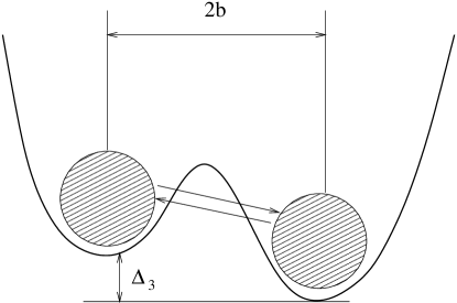
FIG. 1.: Schematic representation of atomic two-level system (TLS).

The corresponding Hamiltonian has the form

$$H = H_{e}+V_{1}\hat{\tau_{1}}\left(\psi^{\dagger}\left({\bf b}\right)\psi\left(-{\bf b}\right)+\psi^{\dagger}\left(-{\bf b}\right)\psi\left({\bf b}\right)\right)$$ (3)

$$+ V_{3}\hat{\tau_{3}}\left(\psi^{\dagger}\left({\bf b}\right)\psi\left({\bf b}\right)-\psi^{\dagger}\left(-{\bf b}\right)\psi\left(-{\bf b}\right)\right),$$ (4)

where $H_{e}$ describes free electrons, and $\hat{\tau_{1}}$ and $\hat{\tau_{3}}$ are Pauli matrices operating in the two-state Hilbert space of the TLS. $V_{1}$ is the amplitude of the “pseudospin-flip” process whereby the TLS tunnels between its two states accompanied by the transfer of an electron from ${\bf b}$ to $-{\bf b}$ or vice versa. $V_{3}$ is the position-dependent interaction between the TLS and electrons. The summation over physical spin is implied in the terms bilinear in electronic annihilation and creation operators $\psi$ and $\psi^{\dagger}$. Terms proportional to $\hat{\tau_{2}}$ are absent in the Hamiltonian because of the combined effect of the invariance under time reversal and locality [21]. Note that the apparently non-local term proportional to $\hat{\tau_{1}}$ in Eq. (3) is an artifact of the approximation neglecting the full momentum dependence of the coupling $V_{1}$.

The Hamiltonian in Eq. (3) can be cast in the form of Eq. (1) with corresponding couplings [30] $J_{3}=\left(2\pi p_{F}b/\sqrt{3}\right)V_{3}$ and $J_{1}=2\pi V_{1}$. The channel quantum numbers in Eq. (1) would then refer to physical spin, while spin quantum numbers correspond to the impurity atom and electronic excitations being located at either of the TLS potential minima, or, depending on the choice of the basis, to different parity eigenstates. Anisotropy of the couplings is unlikely to occur in (hypothetic) magnetic realizations of this model, while TLS realizations generically possess strong anisotropy [21].

The disordered environment is modeled by adding to the Hamiltonian in Eq. (1) the term

$$H_{\rm dis}=H_{c}+H_{s}=\int d{\bf r}\left[U_{c}\left({\bf r}\right)\hat{n}\left({\bf r}\right)+{\bf U}_{s}\left({\bf r}\right)\cdot\hat{\mathchoice{{\hbox{\boldmath$\displaystyle\sigma$}}}{{\hbox{\boldmath$\textstyle\sigma$}}}{{\hbox{\boldmath$\scriptstyle\sigma$}}}{{\hbox{\boldmath$\scriptscriptstyle\sigma$}}}}\left({\bf r}\right)\right],$$ (5)

where $\hat{n}$ and $\hat{\mathchoice{{\hbox{\boldmath$\displaystyle\sigma$}}}{{\hbox{\boldmath$\textstyle\sigma$}}}{{\hbox{\boldmath$\scriptstyle\sigma$}}}{{\hbox{\boldmath$\scriptscriptstyle\sigma$}}}}$ are the charge- and spin-density operators of the conduction electrons, and $U_{c}$ and ${\bf U}_{s}$ are the corresponding random potentials. Formally, the disorder Hamiltonian $H_{\rm dis}$ introduces two additional energy scales into the problem – the inverse scattering time $\tau^{-1}$ and the inverse spin-scattering time $\tau_{s}^{-1}$.

Before proceeding further, we will comment briefly on the role of the charge disorder term $H_{c}$ in $H_{\rm dis}$. It has been discussed in numerous works including Refs. [5, 6, 7, 8, 9, 10]. A related self-consistent model for the case of a finite concentration of Kondo impurities has been considered in Ref. [12]. This term affects only the charge degree of freedom, and one of its effects is to randomize the Kondo temperature $T_{K}$. In systems of lower dimensionality, it can also produce singular corrections to the energy dependence of thermodynamic and transport coefficients in the perturbative high-temperature regime. Incorporating charge disorder into the description of the low-temperature ($T<T_{K}$) regime of the Kondo effect has not been achieved so far. However, it has been argued in Ref. [6] that, in the one-channel magnetic case, the basic nature of the ground state as a local Fermi liquid would not change.

In the context of the magnetic Kondo effect, we will only consider the role of spin disorder. Furthermore, we will restrict the consideration to the case of the ordinary one-channel effect, both because multichannel magnetic realizations have not been unambiguously observed, and because the consideration of the renormalization of splittings (Section III) cannot be transferred to the case $n>2$. [The renormalization of splittings in the $n=2$ case is discussed in Section III. The results for a hypothetical magnetic isotropic $n=2$ case can be obtained by a simple change $\gamma_{m}\rightarrow 2\gamma_{m}$ in Eq. (11).]

In the orbital two-channel realization of the Kondo effect, the roles of spin and orbital degrees of freedom are partially interchanged. The potential scattering term $H_{c}$ in Eq. (5) will produce a contribution analogous to the spin-scattering term, $H_{s}$, when Eq. (3) is transformed into the form of Eq. (1) [29]. In what follows, the term “spin scattering” is understood to apply either to physical spin in the context of magnetic Kondo effect, or to “pseudospin” constructed out of electronic states of different parity in the context of the orbital two-channel realization.

Our choice of model for disorder assumes that breaking of the spin symmetry is due to a well-defined set of scatterers present in the system. The scatterers couple to the spin degrees of freedom, e.g. “frozen” magnetic impurities in the magnetic one-channel case, or ordinary non-magnetic defects in the orbital two-channel case. Replacing such a set of defects by a continuous random Gaussian-distributed potential, as is frequently done in transport calculations, is not warranted here because the distribution of splittings $\Delta$ is non-universal. That is, its form depends on the choice of the distribution function for the random potentials $U_{c}\left({\bf r}\right)$ and ${\bf U}_{s}\left({\bf r}\right)$, and therefore a more realistic model is required.

In the model of isolated scatterers spin disorder is given by

$${\bf U_{s}}\left({\bf r}\right)=g\sum_{i}{\bf S}_{i}\delta\left({\bf r}-{\bf r}_{i}\right),$$ (6)

where ${\bf S}_{i}$ are randomly oriented frozen spins located at randomly selected points ${\bf r}_{i}$, and $g$ is the corresponding exchange coupling constant. The distribution of each of ${\bf S}_{i}$ is assumed isotropic and is given by

$${\cal P}_{S}\left({\bf S}\right)=\frac{1}{2\pi}\delta\left(1-{\bf S}^{2}\right).$$ (7)

In the TLS case, we use a slightly more general expression, allowing for scatterers of finite size:

$$U_{c}\left({\bf r}\right)=\sum_{i}U\left({\bf r}-{\bf r}_{i}\right).$$ (8)

Since “spin” degrees of freedom in this case are a subset of orbital degrees of freedom, the above expression contains both charge disorder and “spin” disorder terms. We will only concentrate on the effect of the latter.

Below we will restrict our consideration to the case of rotationally invariant potentials $U$, so that the corresponding scattering matrix ${\cal T}$ can be reduced to the diagonal form ${\cal T}={\mathrm{diag}}\left({\cal T}_{l}\right)$, where ${\cal T}_{l}$ can be expressed in terms of phase shifts $\eta_{l}$ for each value of the orbital angular momentum as

$${\cal T}_{l}=-\frac{1}{\pi\nu}e^{i\eta_{l}}\sin\eta_{l}.$$ (9)

The coordinates ${\bf r}_{i}$ of $N$ impurities are drawn from a uniform distribution ${\cal P}_{r}\left(\left\{{\bf r}_{i}\right\}\right)=1/{\cal V}^{N}$ where ${\cal V}$ is the total volume of the sample. The calculations are performed in the limit $N,{\cal V}\rightarrow\infty$ with the concentration $c=N/{\cal V}$ kept finite. It is assumed that the concentration is small in the sense that the typical inter-impurity distance $d\sim c^{-1/3}$ is much larger than the Fermi wavelength $\lambda_{F}=2\pi/p_{F}$, which implies, in the magnetic case, $E_{F}\tau_{s}\gg 1$, and $E_{F}\tau\gg 1$ in the TLS case, where $E_{F}$ and $p_{F}$ are the Fermi energy and Fermi momentum, respectively. The effective “spin” scattering time in the TLS case is also of the order of $\tau$, and we will keep the notation $\tau_{s}$ for it.

A Splitting of Internal States of Dynamic Impurity by Spin Scattering.

What is the main effect of spin scattering on the behavior of a Kondo impurity? Even though a non-zero value of $\tau_{s}^{-1}$ means that “spin memory” of electrons has a finite lifetime, the spin-flip processes at the location of the Kondo impurity still lead to logarithmic divergences in the high-temperature perturbative expansion (see Appendix A). In fact, $\tau_{s}^{-1}$ does not directly compete with the Kondo temperature $T_{K}$. Nevertheless, spin scattering can change the low-temperature behavior of an impurity by introducing an effective splitting, $\Delta$, between its internal states.

To understand qualitatively why finite $\tau_{s}^{-1}$ does not by itself destroy the Kondo effect, consider the underlying Anderson model for a magnetic impurity. In this description, the Kondo effect is reflected in the logarithmic divergence of the perturbative contributions to the impurity electron self-energy at $E_{F}$. There are two processes that contribute to this self-energy: tunneling of an impurity electron into the conduction band, and the reverse process, tunneling of a conduction electron onto the impurity. Both of these contributions are logarithmically divergent at $E_{F}$ but with opposite signs. For an impurity without on-site interactions, the two terms cancel and there is no Kondo effect. Interactions remove this cancelation, essentially because an occupied site can only decay in one way – by an electron tunneling out (double occupancy is forbidden or strongly suppressed by Coulomb repulsion), while an unoccupied site can decay in two ways – by an electron of either spin tunneling in. The appearance of a finite $\tau_{s}^{-1}$ may change slightly the relative tunneling rates for spin-up and spin-down electrons, but it cannot significantly change the factor of two difference between the rate of decay of an occupied and an unoccupied site. Hence $\tau_{s}^{-1}$ does not directly destroy the logarithmic divergences in perturbation theory associated with the Kondo effect.

FIG. 2.: (a) The dominant contribution to the effective splitting $\Delta$. The solid line represents the conduction electron Green function, and the broken line represents pseudofermions. The dot represents the interaction vertex $J$, and the cross corresponds to impurity scattering. (b) The leading logarithmic order (parquet) contribution to the splitting. (c) The sum of parquet diagrams. The large dot represents the renormalized (in parquet approximation) scattering amplitude $J_{R}$. (d) Renormalization of splitting.

Importantly, however, the main effect of spin scattering is to break time-reversal invariance and hence induce a splitting $\Delta$ between the two spin states of the Kondo impurity. The splitting results from the appearance of a random non-zero quantum-mechanical expectation value of the local spin density of states $\mathchoice{{\hbox{\boldmath$\displaystyle\sigma$}}}{{\hbox{\boldmath$\textstyle\sigma$}}}{{\hbox{\boldmath$\scriptstyle\sigma$}}}{{\hbox{\boldmath$\scriptscriptstyle\sigma$}}}\left(\epsilon\right)$ at the impurity site. The coupling of $\mathchoice{{\hbox{\boldmath$\displaystyle\sigma$}}}{{\hbox{\boldmath$\textstyle\sigma$}}}{{\hbox{\boldmath$\scriptstyle\sigma$}}}{{\hbox{\boldmath$\scriptscriptstyle\sigma$}}}\left(\epsilon\right)$ to the dynamic impurity via $J$ is responsible for breaking the energy degeneracy between different orientations of the impurity spin. In the diagrammatic language, the splitting is associated not with the modification of the standard set of logarithmic diagrams, but rather with proliferation of a new set of diagrams which were forbidden by ${\rm SU}(2)$ and time-reversal symmetries in the absence of spin disorder. The leading contribution to $\Delta$ in perturbation theory in the coupling strength $J$ is shown in Fig. 2a. The energy scale established by $\Delta$ serves as a cut-off of all logarithmic divergences in the perturbation theory in $J$.

Formally, the main effect of spin disorder is to generate a self-energy term which is essentially energy-independent, and can be reinterpreted as a contribution to the effective impurity Hamiltonian. It is a Hermitian $2\times 2$ matrix in the space of impurity states. In the magnetic case, it is convenient to expand this matrix in the basis of Pauli matrices as

$$H_{\mbox{\text{e}ff}}=\sum_{\alpha=1}^{3}\Delta_{\alpha}\hat{\tau}^{\alpha},$$ (10)

where the $\Delta_{\alpha}$ denote the components of the impurity energy in this basis.

The discussion presented so far does not distinguish between the one- and two-channel cases. This is natural since the high-temperature diagrammatic expansions in the two cases have identical structures, and differ only in factors of $2$ (from the two channels) for closed electronic loops. If the Kondo temperature $T_{K}<\Delta$, spin-flip processes are suppressed at $T<\Delta$, the strongly correlated state is never formed, and below $\Delta$ all temperature dependences are of the Fermi liquid type. If, however, $T_{K}>\Delta$, the behavior of the one- and two-channel Kondo systems is very different. In the one-channel case a non-zero but small $\Delta$ is equivalent to a weak polarizing field acting on the Kondo impurity, resulting in finite but small changes in the values of impurity susceptibility and conductance. However, since these quantities depend on $T_{K}$, which is itself altered in a random way by disorder, no significant experimental consequences follow from a small splitting $\Delta<T_{K}$.

Conversely, in the two-channel case when $\Delta\neq 0$ there appear two distinct low-temperature regimes. A non-Fermi-liquid regime survives in the interval between $T^{*}<T<T_{K}$, where $T^{*}$ is a new characteristic temperature, $T^{*}=\Delta^{2}/2\pi T_{K}$ [31, 32, 33]. A Fermi-liquid regime emerges below $T^{*}$. Hence, the low-temperature properties of an ensemble of two-channel Kondo impurities will explicitly depend on the distribution of splittings $\Delta$.

If $\Delta>T_{K}$, a non-Fermi-liquid regime does not exist, and at temperatures below $\Delta$ the splitting becomes the only relevant energy scale. In other words, the TLS (or, rather, the composite object comprised of the TLS and correlated electrons) becomes frozen in its lowest energy state. Excitations above this state result in $T^{2}$ dependences which blend with other Fermi-liquid effects that are always present. As was demonstrated by Moustakas and Fisher [30], a generic set of TLS parameters almost always corresponds to $\Delta>T_{K}$. In order to observe the non-Fermi-liquid square-root scaling behavior, the parameters of the Hamiltonian have to be fine tuned [34].

The distribution of splittings in the ordinary (one-channel) magnetic case has a simple form (Ref. [16], Section III)

$${\cal P}_{m}\left(\Delta\right)=\frac{4\gamma_{m}}{\pi}\frac{\Delta^{2}}{\left(\Delta^{2}+\gamma_{m}^{2}\right)^{2}},$$ (11)

where $\gamma_{m}=\left(2\pi^{2}c/3p_{F}^{3}\right)Jg\nu^{2}E_{F}$ is a constant which determines the scale for the typical values of $\Delta$. It is proportional to the strength of the dimensionless Kondo coupling $\nu J$, where $\nu$ is the density of states at the Fermi level, and to the magnitude of spin scattering $g$ [Eq. (6)]. The quadratic suppression of ${\cal P}_{m}$ at small $\Delta$ results from the fact that $\Delta^{2}$ is a sum of three random variables $\Delta_{\alpha}^{2}$, each possessing a smooth distribution near $\Delta_{\alpha}=0$. Crucially, the Kondo temperature $T_{K}\sim E_{F}e^{-1/\left(\nu J\right)}$ is exponentially small, so even in systems with weak magnetic disorder ($c/p_{F}^{3},\,\nu g\ll 1$) $\gamma_{m}$ may be comparable to $T_{K}$.

In the orbital two-channel Kondo case, we will show in Section III that ${\cal P}\left(\Delta\right)$ is described by a more complicated analytical expression,

$${\cal P}\left(\Delta\right)=\int_{0}^{2\pi}\frac{d\theta}{2\pi}\frac{K\left(\theta\right)}{\sqrt{K_{1}K_{3}}}\frac{\Delta\gamma\left(\theta\right)}{\left[\Delta^{2}+\gamma^{2}\left(\theta\right)\right]^{3/2}},$$ (12)

where $K\left(\theta\right)=\left(\cos^{2}\theta/K_{1}+\sin^{2}\theta/K_{3}\right)^{-1}$, $\gamma\left(\theta\right)=\displaystyle{\frac{2\pi c}{3p_{F}^{3}}\sqrt{\frac{K\left(\theta\right)}{2}}F\left(\theta\right)}$, and

$$F\left(\theta\right)=1+\frac{\cos^{2}\theta}{\left|\sin\theta\right|}\ln\left(\left|\tan\theta\right|+\frac{1}{\left|\cos\theta\right|}\right).$$ (13)

The constants $K_{1}$ and $K_{3}$ depend on the strength of electronic coupling to the TLS and static scatterers,

$$K_{1}=2\left(E_{F}V_{1}\nu t\right)^{2},\,\,\,K_{3}=2\left(E_{F}V_{3}\nu t\right)^{2}\left(2p_{F}b\right)^{2},$$ (14)

where the scatterer strength $t$ is expressed in terms of the scattering phase shifts $\eta_{l}$ introduced in Eq. (9):

$$t=\sum_{l}\left(-1\right)^{l}\left(2l+1\right)\sin\left(2\eta_{l}\right).$$ (15)

The function $\gamma\left(\theta\right)$ is the analog of the parameter $\gamma_{m}$ introduced in the magnetic case.

In the asymptotic limit $\Delta\gg\displaystyle{\frac{c}{p_{F}^{3}}}\max\left\{\sqrt{K_{1}},\sqrt{K_{3}}\right\}$ the above expression simplifies to

$${\cal P}\left(\Delta\right)\sim\frac{\sqrt{2}cK_{1}K_{3}}{3p_{F}^{3}\Delta^{2}}\int_{0}^{2\pi}\frac{F\left(\theta\right)d\theta}{\left(K_{1}\sin^{2}\theta+K_{3}\cos^{2}\theta\right)^{3/2}}.$$ (16)

The distribution function in Eq. (16) has the same asymptotic $\Delta^{-2}$ behavior as Eq. (11) for large $\Delta$. However, the full distribution function given by Eq. (12) is linear rather than quadratic at small $\Delta$ because, in the absence of $\hat{\tau_{2}}$ terms in the bare Hamiltonian, $\Delta^{2}$ is a sum of two rather than three random variables. In physical models of TLS the couplings are usually related via $V_{1}\sim V_{3}\left(2p_{F}b\right)^{2}$ (see Ref. [21]). This typically corresponds to $K_{3}\gg K_{1}$, so that the distribution function acquires a third asymptotic region. It extends between the sharp maximum at $\Delta\sim\left(c/p_{F}^{3}\right)\sqrt{K_{1}}\sim\left(\nu V_{1}ct/p_{F}^{3}\right)E_{F}$ and the beginning of the $\Delta^{-2}$ decay at $\Delta\sim\left(c/p_{F}^{3}\right)\sqrt{K_{3}}\sim\left(\nu V_{3}ct/p_{F}^{3}\right)E_{F}$, and corresponds to approximately linear decay of the distribution function from a constant value. If $K_{1}\approx K_{3}$, the intermediate asymptotic regime disappears.

The graph of ${\cal P}\left(\Delta\right)$ for the strongly anisotropic regime, corresponding to the choice of parameters discussed in Appendix B ($c/p_{F}^{3}\approx 10^{-4}$, $K_{3}=.38E_{F}^{2}$, $K_{1}=3.7\cdot 10^{-5}E_{F}^{2}$), is shown in Fig. 3. The isotropic case ($K_{1}=K_{3}=.5E_{F}^{2}$) is shown in the top inset. Note that both crossovers between asymptotic regimes in the main graph occur at values of $\Delta$ which are significantly smaller than the r.m.s. splitting quoted in Ref. [11] (see also Ref. [35]): $\left\langle\Delta^{2}\right\rangle^{1/2}\sim 100\mathrm{K}\sim 10^{-3}E_{F}$, where the value $E_{F}\approx 8\cdot 10^{4}K$ for copper has been used.

FIG. 3.: The distribution function of splittings $\Delta$. The parameters of the distribution function are chosen as follows(see Appendix B): $c/p_{F}^{3}=10^{-4}$, $K_{3}=.38E_{F}^{2}$, $K_{1}=3.7\cdot 10^{-5}E_{F}^{2}$; the Fermi energy of Cu is $E_{F}=8\cdot 10^{4}$K. Insets: (a) Isotropic case $K_{1}=K_{3}=.5E_{F}^{2}$. (b) Distribution of the crossover temperature $T^{*}$; parameter regime is the same as in the main graph; $T_{K}\approx 8.2{\mathrm{K}}$.

Assuming that fluctuations of the Kondo temperature $T_{K}$ can be neglected (see Appendix C), the distribution of $T^{*}$ – the temperature at which the crossover from non-Fermi-liquid to Fermi-liquid behavior occurs – is easily inferred from Eq. (12):

$$\widetilde{\cal P}\left(T^{*}\right)=\int_{0}^{2\pi}\frac{d\theta}{4\pi}\frac{K\left(\theta\right)}{\sqrt{K_{1}K_{3}}}\frac{\gamma\left(\theta\right)/\sqrt{2\pi T_{K}}}{\left[T^{*}+\gamma^{2}\left(\theta\right)/2\pi T_{K}\right]^{3/2}}.$$ (17)

This expression is applicable only for $T^{*}\ll T_{K}$, where the relationship $T^{*}=\Delta^{2}/2\pi T_{K}$ holds. The graph of $\widetilde{\cal P}\left(T^{*}\right)$ is shown in the bottom inset in Fig. 3. The corresponding limiting behaviors are

$$\widetilde{\cal P}\left(T^{*}\right)\propto\left\{\begin{array}[]{l}\displaystyle{\frac{4T_{K}}{\sqrt{K_{1}K_{3}}}\left(\frac{2\pi c}{3p_{F}^{3}}\right)^{-2}\int_{0}^{\pi/2}\frac{d\theta}{F^{2}\left(\theta\right)}},\\ \quad\quad\quad\quad\quad T^{*}<\left(c/p_{F}^{3}\right)^{2}{\mathrm{min}}\left(K_{1},K_{3}\right)/T_{K},\\ \displaystyle{\frac{2\pi c/3p_{F}^{3}}{\sqrt{\pi^{3}T_{K}T^{*3}}}\int_{0}^{\pi/2}d\theta\frac{K^{3/2}\left(\theta\right)F\left(\theta\right)}{\sqrt{K_{1}K_{3}}}},\\ \quad\quad\left(c/p_{F}^{3}\right)^{2}{\mathrm{max}}\left(K_{1},K_{3}\right)/T_{K}<T^{*}<T_{K},\end{array}\right.$$ (18)

In the intermediate regime $\left(c/p_{F}^{3}\right)^{2}K_{1}/T_{K}<T^{*}<\left(c/p_{F}^{3}\right)^{2}K_{3}/T_{K}$ the distribution function $\widetilde{\cal P}\left(T^{*}\right)$ is proportional to $1/\sqrt{T^{*}}$. Both the intermediate and the far asymptotic regimes may not exist if the corresponding boundaries become comparable to, or larger than, $T_{K}$.

B Relevance of Disorder to Two-Channel-Kondo-Model Interpretation of Zero-Bias Anomalies.

If the parameters of TLS are randomly drawn from a certain distribution, the net contribution to conductance $\Delta G_{N}\left(T\right)$ from $N$ TLS can be approximated as

$\displaystyle\Delta G_{N}\left(T\right)\approx N\left\langle G\right\rangle+O\left(\sqrt{N}\right),$

where $\left\langle G\right\rangle$ is the contribution of a single TLS averaged over the distribution of $T^{*}$. It was estimated in Ref. [17] that at least 10 separate TLS in the vicinity of the nanoconstriction, and up to 40 in some samples, must be present in order to explain the observed magnitude of the zero-bias anomaly. In this regime the second term on the right-hand side in the above expression would manifest itself as noise on the experimental curves, and hence can be neglected. A scaling ansatz for the anomaly in the zero-bias conductance due to a single TLS can be represented at $T<T_{K}$ as $\Delta G(T)=CT^{1/2}\Upsilon(T^{*}/T)$, where $C$ is a constant and $\Upsilon$ is a smooth function with the limiting behavior $\Upsilon(0)=1$ and $\Upsilon(x\gg 1)\rightarrow 0$. The signal from $N$ TLS is then written as

$$\Delta G_{N}\left(T\right) = NCT^{1/2}\int\widetilde{\cal P}\left(T^{*}\right)\Upsilon\left(T^{*}/T\right)dT^{*}$$ (20)

$$= NCT^{3/2}\int\widetilde{\cal P}\left(xT\right)\Upsilon\left(x\right)dx,$$ (21)

where $x=T^{*}/T$, and $\widetilde{\cal P}\left(T^{*}\right)$ is a normalized distribution. The function $\Upsilon\left(x\right)$ reflects “freezing out” of some impurity degree of freedom, and is likely to decay exponentially at large $x$. Thus the convergence of the above integral at large $x$ is provided by either $\Upsilon$ or $\widetilde{\cal P}$ depending on the temperature.

It has been conjectured in Ref. [20] that the observed $T^{1/2}$ scaling of $G_{N}$ may be consistent with the existence of a distribution of splittings because of an auto-selection process, in which only impurities with sufficiently small $\Delta$ contribute to conductance. Such a scenario would imply that the integral in Eq. (20) could be approximated as

$$\Delta G_{N}\left(T\right)\approx NCT^{3/2}\Upsilon\left(0\right)\int\widetilde{\cal P}\left(xT\right)dx,$$ (22)

resulting in $\Delta G_{N}=NCT^{1/2}$ by virtue of the normalization of $\widetilde{\cal P}$. However, this approximation is only valid if $\widetilde{\cal P}\left(T^{*}\right)$ is peaked so sharply that the integral in Eq. (20) is not much different from its value in the limiting case $\widetilde{\cal P}\left(T^{*}\right)\propto\delta\left(T^{*}\right)$. We will now consider under what circumstances such a behavior of $\widetilde{\cal P}\left(T^{*}\right)$ is possible, and what consequences a different behavior of $\widetilde{\cal P}\left(T^{*}\right)$ would have.

Randomly formed TLS in metallic glasses typically have a broad distribution of asymmetries $\Delta_{z}$ even in the absence of electronic disorder [38]. Neglecting contributions from random $\Delta_{x}$ at first, we can write ${\cal P}\left(\Delta\right)=1/W_{z}$, where $W_{z}$ is independent of $\Delta$ in the region of interest. The corresponding distribution of $T^{*}$ is $\widetilde{\cal P}\left(T^{*}\right)=\sqrt{\pi T_{K}/2T^{*}}/W_{z}$, and consequently $\Delta G_{N}$ must display a linear in temperature behavior,

$\displaystyle\Delta G_{N}=NC\sqrt{\frac{\pi T_{K}}{2W_{z}^{2}}}T\int_{0}^{\infty}\frac{dx}{\sqrt{x}}\Upsilon\left(x\right).$

Non-zero values of $\Delta_{x}$ distributed with a width $W_{x}<W_{z}$ would only exacerbate the discrepancy with the experimentally observed $\Delta G_{N}\sim T^{1/2}$ behavior: specifically, the distribution of $\Delta$ would acquire a linear dip at $\Delta<W_{x}$, yielding a flat distribution of $T^{*}$, leading in turn to $\Delta G_{N}\left(T\right)\sim T^{3/2}$ from the integral in Eq. (20). Thus in order for the Kondo effect in its orbital two-channel realization to be the cause of the observed $T^{1/2}$ scaling, one must assume a set of nearly degenerate TLS, at least before disorder is taken into account. Glassiness as a source of TLS in Ralph-Buhrman samples must, therefore, be ruled out.

Let us now turn to the case when electronic disorder is the only source of TLS splitting, i.e. the TLS are assumed to be formed by some mechanism which, in the absence of coupling to conduction electrons, ensures their degeneracy. The analytic form for the distribution of $T^{*}$, Eq. (17), can be substituted in Eq. (20) together with an exponential ansatz $\Upsilon\left(x\right)=e^{-x}$. Using the available experimental data to determine the parameters of the distribution $\widetilde{\cal P}\left(T^{*}\right)$ in Eq. (17) is not straightforward, and is discussed in detail in Appendix B. Integrating over $x$ we obtain the following integral representation for the TLS contribution to conductance:

$$\Delta G_{N}\left(T\right)=NCT^{1/2}\int_{0}^{2\pi}\frac{d\theta}{2\pi}\frac{K\left(\theta\right)}{\sqrt{K_{1}K_{3}}}$$ (23)

$$\times\left\{1-\frac{\gamma\left(\theta\right)}{\sqrt{2T_{K}T}}\exp\left[\frac{\gamma^{2}\left(\theta\right)}{2\pi T_{K}T}\right]{\mathrm{erfc}}\left[\frac{\gamma\left(\theta\right)}{\sqrt{2\pi T_{K}T}}\right]\right\}.$$ (24)

The remaining integral over $\theta$ is performed numerically, and the resulting graph for the temperature dependence of $\Delta G_{N}$ is shown in Fig. 4.

FIG. 4.: Temperature dependence of the change in conductance due to scattering by an ensemble of TLS, based on Eq. (23). The solid line is the result of numerical evaluation, and the dot-dash line is the linear fit $\ln\left(\Delta G_{N}/NC\right)=-4.83+0.84\ln\left(T/T_{K}\right)$.

As discussed in Appendix B, electronic disorder is assumed to be caused by strongly scattering non-equilibrium vacancies. The plot in Fig. 4 does indicate a behavior close to a power law. However, the best fit in the region between $.05T_{K}<T<.5T_{K}$, corresponding to the interval $.4K<T<4K$ for $T_{K}\approx 8K$, gives $\Delta G_{N}\propto T^{\alpha_{\mathrm{fit}}}$ with $\alpha_{\mathrm{fit}}\approx.84$. The deviation from the $T^{1/2}$ behavior expected for degenerate TLS is rather significant. While the measured exponent in the temperature dependence of zero-bias conductance does show deviations from $\alpha=1/2$, they do not exceed $.25$ (Ref. [20]), so that the value $.84$ clearly lies outside the experimental error.

This result can be understood better by examining under what conditions Eq. (22) can be valid. Let us assume, for simplicity, that $\widetilde{\cal P}$ is characterized by a single parameter, its width $W$. Formally, Eq. (22) can be used when $T\ll W$. Let us consider a hypothetical case of a sufficiently sharp distribution, e.g. a Gaussian, $\widetilde{\cal P}=\sqrt{2/\pi W^{2}}\exp\left[-T^{*2}/2W^{2}\right]$. Substituting this form into Eq. (20) we find that in the temperature region $W<T<10W$, the best fit gives a power-law exponent of approximately .7, while the asymptotic behavior .5 is approached within a 10$\%$ accuracy in the region $10W<T<20W$. Thus, even in the case of a sharp distribution, the relation $T\ll W$ has to be understood as implying at least an order-of-magnitude difference. Returning to the actual distribution Eq. (12), we note that it is a much broader function with a power-law $1/T^{*3/2}$ tail so that the condition for the validity of Eq. (22) is even stricter. At the same time, the larger of the two parameters controlling the width of $\widetilde{\cal P}\left(T^{*}\right)$ is $W\sim\left(c/p_{F}^{3}\right)^{2}K_{3}/T_{K}\sim 3{\mathrm{K}}\sim.3T_{K}$, so that the asymptotic condition $W\ll T$ can never be satisfied for temperatures below $T_{K}$.

It should be observed that the most optimistic choice of parameters for the two-channel Kondo interpretation, corresponding to scattering by non-equilibrium vacancies, leads to an estimate for the concentration of defects $c/p_{F}^{3}\approx 10^{-4}$. Using such a choice of parameters to support the two-channel Kondo interpretation also meets with a difficulty concerning the fraction of defects which form two-level systems. Indeed, using the estimate made in Ref. [17] of up to 40 separate TLS in the vicinity of the nanoconstriction, the corresponding estimate for the density of active TLS is found in Ref. [20] to be $10^{-4}/\mathrm{atom}$, or $c_{\mathrm{active}}/p_{F}^{3}\approx 2\cdot 10^{-5}$. It can be assumed that TLS with $T^{*}<T_{0}$, where $T_{0}$ is the appropriately chosen cut-off temperature, are active. Then the ratio of the concentration of active TLS to their total concentration $c_{\mathrm{TLS}}$ is given by

$$\frac{c_{\mathrm{active}}}{c_{\mathrm{TLS}}}=\int_{0}^{T_{0}}\widetilde{\cal P}\left(T^{*}\right)dT^{*}.$$ (25)

Choosing $T_{0}\approx.8K$, which is a slightly generous assumption, since the $T^{1/2}$ behavior is traced experimentally down to temperatures $T\approx.4K$, we find $c_{\mathrm{active}}/c_{\mathrm{TLS}}\approx 0.4$. The total density of TLS is consequently estimated at $c_{\mathrm{TLS}}/p_{F}^{3}\approx\left(1/0.4\right)c_{\mathrm{active}}/p_{F}^{3}\approx 0.5\cdot 10^{-4}$. Comparing this to the above estimate of $c/p_{F}^{3}\approx 10^{-4}$ for the total concentration of defects forces the improbable conclusion that half of all the defects in the constriction are two-level systems. In other words, in order for the auto-selection mechanism to work, the total number of TLS which would be degenerate in the absence of disorder must be so large as to be inconsistent with the results of measurements indicating a rather small overall density of defects in the nanoconstriction. Although indirect, this reasoning serves, in our view, as another indicator of internal consistency problems with the two-channel Kondo interpretation of zero-bias anomalies in Cu nanoconstrictions.

III The distribution of splittings.

A Local Spin in a Spin Glass Environment

The coupling of the conduction electrons to the random spins results in the appearance of a non-zero expectation value of the conduction-electron spin density at a generic point in the sample. When this spin density is coupled to the dynamic impurity, the lowest order effect is to generate a self-energy matrix, whose components $\Delta_{\alpha}$ in the basis of Pauli matrices and to the lowest order in impurity concentration $c$ are (see diagram in Fig. 2a)

$$\Delta_{\alpha}=-iJg\sum_{i}\int\frac{d\epsilon}{2\pi}G^{2}\left(\epsilon;{\bf r}_{i}\right)S_{i}^{\alpha},$$ (26)

where the zero-temperature Green function in the coordinate representation is given by

$$G\left(\epsilon;{\bf r}\right)=-\frac{\pi\nu}{p_{F}r}\exp\left\{i\left(p_{F}r+\frac{\epsilon}{v_{F}}r\right)\mbox{\text{S}gn}\epsilon\right\}.$$ (27)

Note that $\Delta_{\alpha}$ is proportional to the RKKY-induced random spin polarization in direction $\alpha$ at the position of the impurity. To the lowest order in $J$, the distribution of splittings follows the distribution of internal random magnetic fields in spin glasses. The latter has been derived in Ref. [16] using a somewhat simplified RKKY interaction, in which its oscillatory character is modeled by random signs. The derivation below, while reproducing the essential results of Ref. [16] serves primarily to introduce the more technically involved derivation for the non-magnetic two-channel case presented in the next subsection.

Integrating over energy we obtain

$$\Delta_{\alpha}=Jg\nu^{2}\sum_{i}\frac{\pi E_{F}}{\left(p_{F}r_{i}\right)^{3}}\cos\left(2p_{F}r_{i}\right)S_{i}^{\alpha}.$$ (28)

The distribution function of $\Delta=\sqrt{\sum_{\alpha}\Delta_{\alpha}^{2}}$ therefore takes the form

$${\cal P}_{m}\left(\Delta\right)=2\Delta\int\prod_{i}^{N}\frac{d{\bf r}_{i}}{\cal V}\int\prod_{i}^{N}\frac{d{\bf S}_{i}}{2\pi}$$ (29)

$$\times \delta\left(1-{\bf S}_{i}^{2}\right)\delta\left(\Delta^{2}-\frac{K}{2}\sum_{ij}f\left({\bf r}_{i}\right)f\left({\bf r}_{j}\right){\bf S}_{i}{\bf S}_{j}\right),$$ (30)

where $K=2\left(\pi Jg\nu^{2}E_{F}\right)^{2}$ and $f\left({\bf r}_{i}\right)\equiv f_{i}=\displaystyle{\frac{\cos\left(2p_{F}r_{i}\right)}{\left(p_{F}r_{i}\right)^{3}}}$. Exponentiating the second $\delta$-function and introducing a shorthand notation ${\bf F}=\sum_{i}f_{i}{\bf S}_{i}$ we rewrite the distribution function as

$${\cal P}_{m}\left(\Delta\right) = 2\Delta\int\prod_{i}^{N}\frac{d{\bf r}_{i}}{\cal V}\int\prod_{i}^{N}\frac{d{\bf S}_{i}}{2\pi}\delta\left(1-{\bf S}_{i}^{2}\right)$$ (31)

$$\times \int\frac{d\mu}{2\pi}e^{i\mu\Delta^{2}-\frac{i}{2}\mu K{\bf F}^{2}}.$$ (32)

Decoupling the last term in the exponent with the help of a “Hubbard-Stratonovich” transformation we obtain

$${\cal P}_{m}\left(\Delta\right) = 2\Delta\int\prod_{i}^{N}\frac{d{\bf r}_{i}}{\cal V}\frac{d{\bf S}_{i}}{2\pi}\delta\left(1-{\bf S}_{i}^{2}\right)\int\frac{d\mu}{2\pi}e^{i\mu\Delta^{2}}$$ (33)

$$\times \int\frac{d\mathchoice{{\hbox{\boldmath$\displaystyle\lambda$}}}{{\hbox{\boldmath$\textstyle\lambda$}}}{{\hbox{\boldmath$\scriptstyle\lambda$}}}{{\hbox{\boldmath$\scriptscriptstyle\lambda$}}}}{\left(2\pi i\mu K\right)^{3/2}}\exp\left\{\frac{i\mathchoice{{\hbox{\boldmath$\displaystyle\lambda$}}}{{\hbox{\boldmath$\textstyle\lambda$}}}{{\hbox{\boldmath$\scriptstyle\lambda$}}}{{\hbox{\boldmath$\scriptscriptstyle\lambda$}}}^{2}}{2\mu K}-i\mathchoice{{\hbox{\boldmath$\displaystyle\lambda$}}}{{\hbox{\boldmath$\textstyle\lambda$}}}{{\hbox{\boldmath$\scriptstyle\lambda$}}}{{\hbox{\boldmath$\scriptscriptstyle\lambda$}}}{\bf F}\right\}$$ (34)

$$= 2\Delta\int\frac{d\mu}{2\pi}e^{i\mu\Delta^{2}}\int\frac{d\mathchoice{{\hbox{\boldmath$\displaystyle\lambda$}}}{{\hbox{\boldmath$\textstyle\lambda$}}}{{\hbox{\boldmath$\scriptstyle\lambda$}}}{{\hbox{\boldmath$\scriptscriptstyle\lambda$}}}}{\left(2\pi i\mu K\right)^{3/2}}\exp\left\{\frac{i\mathchoice{{\hbox{\boldmath$\displaystyle\lambda$}}}{{\hbox{\boldmath$\textstyle\lambda$}}}{{\hbox{\boldmath$\scriptstyle\lambda$}}}{{\hbox{\boldmath$\scriptscriptstyle\lambda$}}}^{2}}{2\mu K}\right\}$$ (35)

$$\times \left[\int\frac{d{\bf r}}{\cal V}\frac{d{\bf S}}{2\pi}\delta\left(1-{\bf S}^{2}\right)e^{-if\left({\bf r}\right)\mathchoice{{\hbox{\boldmath$\displaystyle\lambda$}}}{{\hbox{\boldmath$\textstyle\lambda$}}}{{\hbox{\boldmath$\scriptstyle\lambda$}}}{{\hbox{\boldmath$\scriptscriptstyle\lambda$}}}{\bf S}}\right]^{N}.$$ (36)

The expression in the square brackets can be transformed as follows:

$$\left[\int\frac{d{\bf r}}{\cal V}\int\frac{d{\bf S}}{2\pi}\delta\left(1-{\bf S}^{2}\right)\exp\left\{-if\left({\bf r}\right)\mathchoice{{\hbox{\boldmath$\displaystyle\lambda$}}}{{\hbox{\boldmath$\textstyle\lambda$}}}{{\hbox{\boldmath$\scriptstyle\lambda$}}}{{\hbox{\boldmath$\scriptscriptstyle\lambda$}}}{\bf S}\right\}\right]^{N}$$ (37)

$$= \left[\int\frac{d{\bf r}}{\cal V}\frac{\sin\left[\left|\mathchoice{{\hbox{\boldmath$\displaystyle\lambda$}}}{{\hbox{\boldmath$\textstyle\lambda$}}}{{\hbox{\boldmath$\scriptstyle\lambda$}}}{{\hbox{\boldmath$\scriptscriptstyle\lambda$}}}\right|f\left({\bf r}\right)\right]}{\left|\mathchoice{{\hbox{\boldmath$\displaystyle\lambda$}}}{{\hbox{\boldmath$\textstyle\lambda$}}}{{\hbox{\boldmath$\scriptstyle\lambda$}}}{{\hbox{\boldmath$\scriptscriptstyle\lambda$}}}\right|f\left({\bf r}\right)}\right]^{N}$$ (38)

$$\approx \exp\left\{-c\int d{\bf r}\left(1-\frac{\sin\left[\left|\mathchoice{{\hbox{\boldmath$\displaystyle\lambda$}}}{{\hbox{\boldmath$\textstyle\lambda$}}}{{\hbox{\boldmath$\scriptstyle\lambda$}}}{{\hbox{\boldmath$\scriptscriptstyle\lambda$}}}\right|f\left({\bf r}\right)\right]}{\left|\mathchoice{{\hbox{\boldmath$\displaystyle\lambda$}}}{{\hbox{\boldmath$\textstyle\lambda$}}}{{\hbox{\boldmath$\scriptstyle\lambda$}}}{{\hbox{\boldmath$\scriptscriptstyle\lambda$}}}\right|f\left({\bf r}\right)}\right)\right\}.$$ (39)

To compute the last integral the following approximation is employed: since the dominant contribution to the distribution function is expected to come from $r\sim d$, it is possible to decouple fast oscillations in $f$ (proportional to $\cos 2p_{F}r$) from the slow decay $\left(p_{F}r\right)^{-3}$. Formally, $f\left({\bf r}\right)$ is replaced with $f\left(\varphi,{\bf r}\right)=\displaystyle{\frac{\cos\varphi}{\left(p_{F}r\right)^{3}}}$ with a simultaneous replacement $\displaystyle{\int d{\bf r}\rightarrow\int d{\bf r}\int\frac{d\varphi}{2\pi}}$. Integration over ${\bf r}$ now gives

$$\exp\left\{-\int\frac{d\varphi}{2\pi}\frac{\pi^{2}c\left|\mathchoice{{\hbox{\boldmath$\displaystyle\lambda$}}}{{\hbox{\boldmath$\textstyle\lambda$}}}{{\hbox{\boldmath$\scriptstyle\lambda$}}}{{\hbox{\boldmath$\scriptscriptstyle\lambda$}}}\right|\left|\cos\varphi\right|}{3p_{F}^{3}}\right\}=\exp\left\{-\frac{2\pi c\left|\mathchoice{{\hbox{\boldmath$\displaystyle\lambda$}}}{{\hbox{\boldmath$\textstyle\lambda$}}}{{\hbox{\boldmath$\scriptstyle\lambda$}}}{{\hbox{\boldmath$\scriptscriptstyle\lambda$}}}\right|}{3p_{F}^{3}}\right\}.$$ (40)

Absorbing $\sqrt{|\mu|K}$ into $\lambda$ we can rewrite the distribution function as

$${\cal P}_{m}\left(\Delta\right)=2\Delta\int\frac{d\mu}{2\pi}e^{i\mu\Delta^{2}}\frac{4\pi}{\left(2\pi i{\mathrm{Sgn}}\mu\right)^{3/2}}$$ (41)

$$\times \int_{0}^{\infty}\lambda^{2}d\lambda\exp\left\{\frac{i{\mathrm{Sgn}}\mu}{2}\lambda^{2}-\frac{2\pi c\sqrt{\left|\mu\right|K}\lambda}{3p_{F}^{3}}\right\}.$$ (42)

Rotating the contour of integration by $\left(\pi/4\right){\mathrm{Sgn}}\mu$ we arrive at

$${\cal P}_{m}\left(\Delta\right)=\int \displaystyle{\frac{d\mu}{2\pi}} e^{i\mu\Delta^{2}}\displaystyle{\sqrt{\frac{2}{\pi}}}\int x^{2}dx\exp\left\{-\frac{1}{2}x^{2}\right.$$ (43)

$$- \left.\frac{2\pi c}{3p_{F}^{3}}\frac{1+i{\mathrm{Sgn}}\mu}{\sqrt{2}}\sqrt{\left|\mu\right|K}x\right\}.$$ (44)

Performing another change of variables $y^{2}=2\left|\mu\right|\Delta^{2}$ and rotating the contour of integration over $y$ we obtain the following integral representation for the distribution function:

$${\cal P}_{m}\left(\Delta\right) = -\left(\frac{2}{\pi}\right)^{3/2}{\mathrm{Re}}\frac{\partial}{\partial\gamma_{m}}\int_{0}^{\infty}xdx\int_{0}^{\infty}dy$$ (45)

$$\times \exp\left\{-\frac{1}{2}\left(x^{2}+y^{2}\right)+i\frac{\gamma_{m}}{\Delta}xy\right\},$$ (46)

where $\gamma_{m}=\displaystyle{\frac{2\pi c}{3p_{F}^{3}}\sqrt{\frac{K}{2}}}$. Using polar coordinates $\left(\rho,\theta\right)$ in the $\left(x,y\right)$ plane and integrating over $\rho$ the distribution function can be rewritten as

$${\cal P}_{m}\left(\Delta\right)=-\frac{2}{\pi}{\rm Re}\frac{\partial}{\partial\gamma_{m}}\int_{0}^{\pi/2}\frac{\cos\theta d\theta}{\left(1-i\displaystyle{\frac{\gamma_{m}}{\Delta}}\sin 2\theta\right)^{3/2}}.$$ (47)

The remaining integral can be performed by elementary means leading to the expression for the distribution function (cf. Ref. [16]) quoted in Eq. (11).

B Non-Magnetic TLS in the Presence of Static Defects

The electronic contribution to the splitting between the energy levels of TLS is determined by the difference between the two eigenvalues of the self-energy matrix [14]

$$\left(\begin{array}[]{*{2}{c}}V_{3}\delta_{++}&V_{1}\delta_{+-}\\ V_{1}\delta_{-+}&-V_{3}\delta_{--}\end{array}\right).$$ (48)

The components of this matrix are expressed in terms of the scattering matrix ${\cal T}$ corresponding to the potential $U\left({\bf r}\right)$ introduced in Eq. (8) as

$$\delta_{++}=- 2i \sum_{i}\int\frac{d\epsilon}{2\pi}\int d{\bf r}\int d{\bf r}^{\prime}G_{\epsilon}\left({\bf r}+{\bf b}\right)$$ (50)

$$\times {\cal T}_{\epsilon}\left({\bf r}-{\bf r}_{i},{\bf r}^{\prime}-{\bf r}_{i}\right)G_{\epsilon}\left({\bf r}^{\prime}+{\bf b}\right),$$ (51)

and similarly for $\delta_{--}$. The off-diagonal term $\delta_{+-}$ is

$$\delta_{+-}=- 2i \sum_{i}\int\frac{d\epsilon}{2\pi}\int d{\bf r}\int d{\bf r}^{\prime}G_{\epsilon}\left({\bf r}+{\bf b}\right)$$ (52)

$$\times {\cal T}_{\epsilon}\left({\bf r}-{\bf r}_{i},{\bf r}^{\prime}-{\bf r}_{i}\right)G_{\epsilon}\left({\bf r}^{\prime}-{\bf b}\right).$$ (53)

The factor of $2$ in front is due to summation over channels – the two orientations of the real spin of the conduction electrons. The resulting electronic contribution to the splitting is

$$\Delta^{2}=V_{3}^{2}\left[{\mathrm{Re}}\left(\delta_{++}-\delta_{--}\right)\right]^{2}+4V_{1}^{2}\left({\mathrm{Re}}\,\delta_{+-}\right)^{2}.$$ (54)

After integrating over $\epsilon$ and approximating $\left|{\bf r}_{i}\pm{\bf b}\right|=r_{i}\pm{\bf b}\cdot{\bf n}_{i}$, ${\bf n}_{i}={\bf r}_{i}/r_{i}$, the distribution function for $\Delta$ is given by an expression analogous to Eq. (28):

$${\cal P}\left(\Delta\right)=2\Delta\int\prod_{i}\frac{d{\bf r}_{i}}{\cal V}\delta\left(\Delta^{2}-\sum_{ij}\frac{K_{1}f_{i}f_{j}+\widetilde{K}_{3}h_{i}h_{j}}{2}\right),$$ (55)

where $h_{i}=h\left({\bf r}_{i}\right)=\displaystyle{\frac{\sin 2p_{F}r_{i}}{\left(p_{F}r_{i}\right)^{3}}}\sin\left(2p_{F}{\bf b}\cdot{\bf n}_{i}\right)$, and constants $K_{1}$, $K_{3}$, and $t$ were defined above in Eqs. (14,15). $\widetilde{K_{3}}$ is related to $K_{3}$ via $K_{3}=\left(2p_{F}b\right)^{2}\widetilde{K_{3}}$.

Following the technique used in the preceding section, the distribution function can be represented as an integral over a Lagrange multiplier $\mu$ and two “Hubbard-Stratonovich” variables $\lambda_{1}$ and $\lambda_{3}$,

$${\cal P}\left(\Delta\right)=2 \Delta \int\frac{d\mu}{2\pi}e^{i\mu\Delta^{2}}\int\frac{d\lambda_{1}d\lambda_{3}}{2\pi i\mu\sqrt{K_{1}\widetilde{K}_{3}}}\exp\left\{i\frac{\lambda_{1}^{2}}{2\mu K_{1}}\right.$$ (56)

$$+ \left.i\frac{\lambda_{3}^{2}}{2\mu\widetilde{K}_{3}}-\frac{4\pi c}{3p_{F}^{3}}u\left(\lambda_{1},\lambda_{3}\right)\right\},$$ (57)

where the function $u$ is defined by an expression analogous to Eq. (37),

$$\frac{4\pi c}{3p_{F}^{3}}u\left(\lambda_{1},\lambda_{3}\right)=c\int d{\bf r}\left[1-\exp\left\{-i\lambda_{1}f\left({\bf r}\right)-i\lambda_{3}h\left({\bf r}\right)\right\}\right].$$ (58)

Integrating over orientations of $\mathbf{n}$, and decoupling fast oscillations in $f$ and $h$, we arrive, in the approximation $\sin 2p_{F}b\approx 2p_{F}b$, at an analogue of Eq. (40):

$$u\left(\lambda_{1},\lambda_{3}\right)=\int_{0}^{\infty}\frac{d\zeta}{\zeta^{2}}\int_{0}^{2\pi}\frac{d\varphi}{2\pi} \left[1-\frac{\sin\left(\lambda_{3}\widetilde{b}\sin\varphi\zeta\right)}{\lambda_{3}\widetilde{b}\sin\varphi\zeta}\right.$$ (59)

$$\times \exp\left\{-i\lambda_{1}\cos\varphi\zeta\right\}\Big{]},$$ (60)

where $\widetilde{b}=2p_{F}b$ and $\zeta=1/\left(p_{F}r\right)^{3}$. Integration over $\varphi$ now gives

$$u\left(\lambda_{1},\lambda_{3}\right)=\frac{2\widetilde{b}\left|\lambda_{3}\right|}{\pi}\!\int_{0}^{\infty}\!\!\frac{d\zeta}{\zeta^{2}}\left[1-\frac{\left|\lambda_{1}\right|\sin\zeta}{\left|\lambda_{3}\right|\widetilde{b}}{\mathrm{K}}_{-1}\left(\frac{\zeta\left|\lambda_{1}\right|}{\widetilde{b}\left|\lambda_{3}\right|}\right)\right],$$ (61)

where $\mathrm{K}_{\nu}$ is the modified Bessel function. Completing the remaining integration over $\zeta$, and rescaling $\widetilde{b}\lambda_{3}\rightarrow\lambda_{3}$ so that $\widetilde{K}_{3}$ in Eq. (56) is replaced with $K_{3}=\widetilde{b}^{2}\widetilde{K}_{3}$, we obtain

$$u\left(x,y\right)=\frac{x^{2}}{\left|y\right|}\ln\frac{\left|y\right|+\sqrt{x^{2}+y^{2}}}{\left|x\right|}+\sqrt{x^{2}+y^{2}}.$$ (62)

Using polar coordinates $\left(\lambda,\theta\right)$ in the $\left(\lambda_{1},\lambda_{3}\right)$ plane, introducing another set of polar coordinates $\left(\rho,\psi\right)$ in the $\left(\lambda,\mu\right)$ plane and integrating over $\rho$ we obtain the following integral representation for the distribution function:

$${\cal P}\left(\Delta\right)=\!\int_{0}^{2\pi}\!\!\!\frac{d\theta}{\pi^{2}\Delta}\frac{K\left(\theta\right)}{\sqrt{K_{1}K_{3}}}{\mathrm{Re}}\,\frac{\partial}{\partial\gamma}\left.\!\int_{0}^{\pi/2}\!\!\!\!\!\frac{d\psi}{i\gamma\sin 2\psi-1}\right|_{\gamma=\frac{\gamma\left(\theta\right)}{\Delta}}.$$ (63)

The final result obtained after integrating over $\psi$, together with the definition of $\gamma\left(\theta\right)$, has been presented in Eq. (12).

C Higher Order Contributions.

The scaling ansatz used in Eq. (20) depends crucially on the shape of the distribution function ${\cal P}$ in the region of small splitting $\Delta$. Thus, the applicability of the above analysis hinges on whether the perturbative calculation of $\Delta$ in the preceding subsection is sufficient for $\Delta$’s smaller than $T_{K}$. Only the lowest order diagram in Kondo coupling has been retained in the calculation so far, and we now turn to the consideration of higher order contributions.

These higher order contributions can be conveniently separated into two classes. The diagrams belonging to the first class (Fig. 2c) correspond to the renormalization of the Kondo scattering amplitude with parquet diagrams, which collect the leading order logarithmic terms. They produce corrections to $\Delta$ which are smaller by powers of the Kondo coupling, and, importantly, unlike the Kondo scattering amplitude itself, do not contain any logarithmically divergent terms. These contributions can therefore be neglected.

Indeed, the contributions of the diagrams belonging to the first class is typified by that of the diagram in Fig. 2b:

$$\delta\Delta_{\alpha} = \left(\nu g\right)\left(\nu J\right)^{2}\sum_{i}\frac{\pi E_{F}}{\left(p_{F}r_{i}\right)^{3}}\cos\left(2p_{F}r_{i}\right)S^{\alpha}_{i}$$ (64)

$$\times \left[\ln\frac{E_{F}}{v_{F}/r_{i}}+\mathrm{Const.}\right]$$ (65)

This expression is valid as long as

$$v_{F}/r_{i}<T_{K},$$ (66)

which, for $T_{K}/E_{F}\sim 10^{-4}$ would be violated only at unphysically small concentrations $c/p_{F}^{3}<10^{-12}$. It is seen that this contribution does not contain any uncontrolled logarithmic divergences. The reason is that the sum of all diagrams of this type can be written in the form of Eq. (26), where the bare scattering amplitude $J$ is replaced with the renormalized amplitude $J_{R}\left(\epsilon,\epsilon\right)$. The renormalized amplitude is singular at small energies, but the singularity is integrable, and after the integration over energies in Eq. (26) it only manifests itself in finite logarithmic terms like the first term in square brackets in Eq. (64). The inequality (66) ensures that the contribution of these terms is small in the parameter $\left(\nu J\right)\ln\frac{E_{F}}{v_{F}/d}\ll 1$, and can be ignored.

In contrast, the diagrams of the second class correspond to a further renormalization of the scattering amplitude by particle-hole pairs, and retain the usual logarithmically divergent factors. These terms were previously analyzed perturbatively using the renormalization group (RG) approach in Ref. [21], where it was established that in anisotropic models the effect of these terms may be to renormalize downwards the effective splitting at the scale just above $T_{K}$. We argue that this analysis cannot be straightforwardly extended through the crossover region into the low-temperature regime. Instead, we show that the effective splitting at temperatures below the Kondo temperature can be deduced from the lowest order perturbative result on the basis of universality properties of the two models under consideration, the one- and two-channel Kondo models. We employ the language of the underlying Anderson model, as it affords a unified description of the high- and low-energy regimes [2].

The simplest diagram of the second class is shown in Fig. 2d. These graphs correspond to linear (in $\Delta$) screening of the splitting by the Kondo interaction. In the perturbative renormalization group analysis by Vladár and Zawadowski [21] it was found that the splitting tends to be renormalized downwards, and in the case of strong anisotropy, at least one component of the splitting may be renormalized significantly,

$\displaystyle\Delta_{x\mathrm{,eff}}\left(T\geq T_{K}\right)\sim\Delta_{x}\left(\frac{\nu J_{1}}{4\nu J_{3}}\right)^{1/4\nu J_{3}}.$

However, the perturbative analysis in Ref. [21] cannot be extended to energy scales below $T_{K}$. An extrapolation of the perturbative RG results from the energy scale $E\geq T_{K}$ to predict the values of $\Delta$ at $T\ll T_{K}$ (Ref. [20]) is unjustified because splitting is a relevant operator in the RG sense.

Let us consider first the isotropic one-channel magnetic case. The perturbative renormalization group calculation of Ref. [21], although formulated in terms of the orbital two-channel Kondo model, can be transferred, with minor modifications, to the one-channel case as well because of the identical structures of the corresponding high-temperature perturbation expansions. When graphs of the type shown in Fig. 2b are neglected, the splitting has the literal meaning of an external magnetic field ${\mathbf{h}}$ acting on the impurity. The unrenormalized impurity Green function has the form

$${\cal G}=\left(\omega-\epsilon_{d}+{\mathbf{h}}\cdot\mathchoice{{\hbox{\boldmath$\displaystyle\sigma$}}}{{\hbox{\boldmath$\textstyle\sigma$}}}{{\hbox{\boldmath$\scriptstyle\sigma$}}}{{\hbox{\boldmath$\scriptscriptstyle\sigma$}}}\right)^{-1},$$ (67)

where $\epsilon_{d}$ is the energy of the singly occupied impurity state. The ground state of the model can be described as an effective Fermi liquid, in which the Green function of the impurity spin retains its form under strong renormalization. The fully renormalized ${\cal G}$ will contain additional self-energy contributions [2],

$${\cal G}=\left[\omega-\epsilon_{d}+i\Gamma/z+\mathchoice{{\hbox{\boldmath$\displaystyle h$}}}{{\hbox{\boldmath$\textstyle h$}}}{{\hbox{\boldmath$\scriptstyle h$}}}{{\hbox{\boldmath$\scriptscriptstyle h$}}}\cdot\mathchoice{{\hbox{\boldmath$\displaystyle\sigma$}}}{{\hbox{\boldmath$\textstyle\sigma$}}}{{\hbox{\boldmath$\scriptstyle\sigma$}}}{{\hbox{\boldmath$\scriptscriptstyle\sigma$}}}-\hat{\Sigma}\left(\omega,\mathchoice{{\hbox{\boldmath$\displaystyle h$}}}{{\hbox{\boldmath$\textstyle h$}}}{{\hbox{\boldmath$\scriptstyle h$}}}{{\hbox{\boldmath$\scriptscriptstyle h$}}}\right)\right]^{-1},$$ (68)

where $\Gamma$ is the width of the Kondo resonance. The self-energy $\hat{\Sigma}=\Sigma_{0}+\mathchoice{{\hbox{\boldmath$\displaystyle\Sigma$}}}{{\hbox{\boldmath$\textstyle\Sigma$}}}{{\hbox{\boldmath$\scriptstyle\Sigma$}}}{{\hbox{\boldmath$\scriptscriptstyle\Sigma$}}}\cdot\mathchoice{{\hbox{\boldmath$\displaystyle\sigma$}}}{{\hbox{\boldmath$\textstyle\sigma$}}}{{\hbox{\boldmath$\scriptstyle\sigma$}}}{{\hbox{\boldmath$\scriptscriptstyle\sigma$}}}$ is expanded at small $\omega$ and $\mathbf{h}$ as

$$\Sigma_{0}\left(\omega,\mathchoice{{\hbox{\boldmath$\displaystyle h$}}}{{\hbox{\boldmath$\textstyle h$}}}{{\hbox{\boldmath$\scriptstyle h$}}}{{\hbox{\boldmath$\scriptscriptstyle h$}}}\right) = \Sigma_{00}+\left(1-\frac{1}{z}\right)\omega+iO\left(\omega^{2}\right),$$ (69)

$$\Sigma = \Sigma^{\prime}_{h}\mathchoice{{\hbox{\boldmath$\displaystyle h$}}}{{\hbox{\boldmath$\textstyle h$}}}{{\hbox{\boldmath$\scriptstyle h$}}}{{\hbox{\boldmath$\scriptscriptstyle h$}}},$$ (70)

where $\Sigma^{\prime}_{h}$ and $z$ are the renormalization constants, and $\Sigma_{00}$ is the constant term which, in the case of symmetric Anderson model, is equal to $\epsilon_{d}$ ensuring that the Kondo resonance is centered at the Fermi energy.

Factoring out the quasiparticle weight $z$, the effective field ${\bf h}_{\mathrm{eff}}$ takes the form

$$\mathchoice{{\hbox{\boldmath$\displaystyle h$}}}{{\hbox{\boldmath$\textstyle h$}}}{{\hbox{\boldmath$\scriptstyle h$}}}{{\hbox{\boldmath$\scriptscriptstyle h$}}}_{\mathrm{eff}}=z\left(1-\Sigma^{\prime}_{h}\right)\mathchoice{{\hbox{\boldmath$\displaystyle h$}}}{{\hbox{\boldmath$\textstyle h$}}}{{\hbox{\boldmath$\scriptstyle h$}}}{{\hbox{\boldmath$\scriptscriptstyle h$}}}.$$ (71)

The perturbative RG calculation of renormalized splitting in Ref. [21] is equivalent to computing the same prefactor $\displaystyle{R\left(\omega\right)=z\left(1-\Sigma^{\prime}_{h}\right)\equiv\frac{1-\partial\Sigma/\partial\mathchoice{{\hbox{\boldmath$\displaystyle h$}}}{{\hbox{\boldmath$\textstyle h$}}}{{\hbox{\boldmath$\scriptstyle h$}}}{{\hbox{\boldmath$\scriptscriptstyle h$}}}}{1-\partial\Sigma/\partial\omega}}$ at a finite frequency $\omega$ (see Eqs. (3.5)-(3.10) in the second of Refs. [21]). The frequency dependence of both derivatives in this region is logarithmic, so that, with logarithmic accuracy, frequency can be identified with energy scale in the RG sense. Such scale-dependent quantities determine the properties of the system at temperatures of the order of the energy scale.

The perturbative RG analysis cannot be continued beyond some intermediate scale $E_{0}\gtrsim T_{K}$, and its usefulness for determining low-temperature properties relies on the assumption that further renormalization from $E\sim E_{0}$ to $E\ll T_{K}$ does not change the value of the renormalized quantity in any essential way. This assumption may be violated when renormalization of relevant operators is considered, as is indeed the case in the models considered here.

At zero temperature, the prefactor in Eq. (71) is just the universal Wilson ratio $R$ (Ref. [2]). Substituting its known value, $R=2$, we obtain a seemingly counterintuitive result that, despite downwards renormalization of splitting at $E>T_{K}$, the splitting is actually increased at $E\ll T_{K}$ by a factor of 2 compared to its bare value. Of course, at zero temperature the role of the weak effective magnetic field acting on the impurity is to polarize the Kondo screened complex (as long as $\Delta\ll T_{K}$), and $\mathchoice{{\hbox{\boldmath$\displaystyle h$}}}{{\hbox{\boldmath$\textstyle h$}}}{{\hbox{\boldmath$\scriptstyle h$}}}{{\hbox{\boldmath$\scriptscriptstyle h$}}}_{\mathrm{eff}}$ induces a “splitting” only in this sense.

To explain the non-monotonic behavior of the effective splitting as a function of energy scale (or temperature), one should note that, in the Anderson model, the renormalization of the splitting is proportional to the ratio of the impurity magnetic susceptibility $\chi$ to $C/T$, where $C$ is the impurity specific heat. This ratio is a non-monotonic function of temperature near $T_{K}$, essentially because of the maximum in the temperature dependence of $C$ at $T\sim T_{K}$.

The Anderson model is less well suited for discussion of anisotropic Kondo models. Nevertheless, anisotropy can be modeled, at the price of additional potential scattering in the corresponding s-d Hamiltonian, by introducing spin-dependent renormalization constants $z_{\alpha}$ and $\Sigma^{\prime}_{\alpha\beta}$. Coupling anisotropy is an irrelevant operator (in both one-channel and two-channel spin-$1/2$ Kondo models, see, e.g. Ref. [31]), and the invariance of the Wilson ratio demands that

$$2=z_{\uparrow}\left(1-\Sigma^{\prime}_{\uparrow\uparrow}\right)=z_{\downarrow}\left(1-\Sigma^{\prime}_{\downarrow\downarrow}\right)=\sqrt{z_{\uparrow}z_{\downarrow}}\left(1-\Sigma^{\prime}_{\uparrow\downarrow}\right).$$ (72)

The choice of only two different renormalization constants $z_{\uparrow}$ and $z_{\downarrow}$ corresponds to $J_{1}=J_{2}\neq J_{3}$ in the Kondo effective Hamiltonian. If the field now is chosen in the $xy$ plane ($h_{\uparrow\downarrow}$ in the above notations), the corresponding value of the self-energy at zero temperature is still

$\displaystyle h_{\uparrow\downarrow\mathrm{eff}}=h_{\uparrow\downarrow}\sqrt{z_{\uparrow}z_{\downarrow}}\left(1-\Sigma^{\prime}_{\uparrow\downarrow}\right)=2h_{\uparrow\downarrow}.$

The temperature dependence of this self-energy may be quite non-monotonic, as the transverse susceptibility deviates strongly from the free-spin value at temperatures above the specific heat maximum.

Let us turn now to the two-channel Kondo case. The above analysis cannot be transferred verbatim because the ground state is not a Fermi liquid, and $T^{*}$ does not have the meaning of the renormalized Fermi-liquid quasiparticle self-energy [39]. In particular, the renormalization factor $R\left(\omega\right)$ can no longer be identified with the Wilson ratio of an Anderson-like model. Nevertheless, the salient features of this analysis survive. Once again, we can identify the self-energy contribution of Fig. 2a with an external field ${\bf h}$ acting on the impurity. The effective field in the high-temperature regime is renormalized downwards, in the anisotropic case strongly [21]. However, in the low-temperature regime the weight of the quasiparticle excitations for which this effective field represents the self-energy is zero, so that this self-energy term does not define any physical low-temperature energy scale. It has been demonstrated recently [39, 40] that impurity thermodynamics in the low-temperature regime can be described in terms of three vector and one scalar Majorana quasiparticles. An external field ${\bf h}$ generates a self-energy contribution for the scalar Majorana fermion $\Sigma_{M}=h^{2}/2\pi T_{K}=T^{*}$ which is universal apart from its dependence on $T_{K}$ [31, 32, 33]. The universality [36] ensures that $T^{*}$ is controlled by the unrenormalized value of $h$, namely the bare splitting $\Delta$.

IV Discussion.

The results of our model calculation of the splitting between the states of magnetic impurities and non-magnetic two-level systems (TLS) in the presence of spin disorder can be summarized as follows. First, the main feature of the distribution functions of the splittings is their strong asymmetry. Formally the distribution functions in Eqs. (11) and (13) do not even possess finite first moments. This is a manifestation of the fact that all the moments of the splittings are dominated by disorder configurations with one or more scatterers located very close to the dynamic impurity. In real systems the shortest possible separation between the dynamic impurity and the nearest scatterer is determined by the lattice spacing. Therefore one has to introduce a short distance, lattice cut-off into the coordinate integration in Eq. (37). In the presence of such a cutoff all the moments are dominated by distances of the order of the cut-off, and thus, for example, the average rms splitting $\displaystyle{\sqrt{\left\langle\Delta^{2}\right\rangle}}$ is of the order of $E_{F}\left(Jg\nu^{2}\right)\sqrt{c/p_{F}^{3}}$ for the magnetic case or $E_{F}\left({\rm max}\left\{V_{1},V_{3}p_{F}b\right\}\right)t\nu\sqrt{c/p_{F}^{3}}$ for the non-magnetic TLS case. These values are larger than the typical ones by a factor of $\sqrt{p_{F}^{3}/c}\sim\left(p_{F}d\right)^{3/2}\gg 1$. This confirms the result obtained independently by D. Cox [41].

Second, since the splitting is the difference between two eigenvalues of a random Hermitian $2\times 2$ matrix, at small splittings one observes the equivalent of level repulsion leading to a vanishing probability density to observe zero splitting. In the non-magnetic TLS case the matrix is real and symmetric, and the suppression is linear rather than quadratic.

The asymmetry of the distribution functions has important implications for the study of the effects of spin disorder on the behavior of Kondo impurities in the crossover and low-temperature regimes. Because of the build-up of many-particle correlations at low temperatures, the effective splitting between the levels of magnetic impurities or TLS, $\Delta_{\rm eff}\left(T\right)$, can be reduced at intermediate temperatures $T\sim T_{K}$ compared to the bare value $\Delta$ (Refs. [21, 30]). Since the distribution of splittings is very asymmetric, with the root-mean-square splitting much larger than the typical value, a proper renormalization analysis would necessarily treat the full distribution rather than just the first few moments. To what extent the distributions found here preserve their shape under renormalization is an open question.

Nevertheless, the zero-temperature behavior of the splitting, or, more precisely, of the corresponding self-energy terms, is dictated by the universality properties of the one- and two-channel Kondo models, and can be extracted directly. This, in turn, made it possible to derive a corresponding temperature dependence of conductance for a collection of two-level systems. We find (cf. Ref. [11]) a $T^{\alpha}$ behavior with $\alpha\approx.84$ in contrast to the $T^{1/2}$ dependence observed experimentally [17, 18, 20]. The concentration of the TLS which must be degenerate (in the absence of disorder) in order to sustain the two-channel Kondo interpretation is also found to be unphysically large. Both these arguments suggest that the two-channel Kondo model does not provide a consistent interpretation of the zero-bias anomalies observed in Ref. [17].

In conclusion, we have computed the distribution functions of splittings of magnetic impurities and non-magnetic two-level systems (TLS) induced by disorder scattering of conduction electrons. In the magnetic case these splittings only appear if the disorder breaks time-reversal symmetry, i.e. if the disorder is itself magnetic. In the non-magnetic case the degeneracy between the levels of a TLS is due to geometric symmetry about its center, and therefore is strongly broken by any type of disorder. We find that the probability distribution of splittings vanishes as a power law at small splittings, making nearly degenerate impurities a rarity. The typical values of splittings are found to be smaller than the average estimated previously in Ref. [11]. However, even in quite clean systems such as the ones studied in the experiments of Ref. [17], the broad profile of the distribution of splittings results in a temperature dependence of the conductance which is substantially different from the square-root law expected in the absence of disorder. Consequently, experimental observation of the square-root temperature and voltage dependences may not be a reliable indicator of two-channel Kondo physics.

A

To illustrate the small effects of spin disorder on the standard logarithmic terms in the perturbation-theory expansion, we consider the well-known lowest-order logarithmic contribution to the spin susceptibility given by the diagram shown in Fig. 5.

FIG. 5.: The lowest order logarithmic contribution to susceptibility in the magnetic Kondo problem. The wavy lines correspond to the external magnetic field.

As in other similar logarithmic diagrams, there appears a set of terms due to the off-diagonal in spin index parts of the Green function. The corresponding analytical expression is

$$\displaystyle{\frac{\delta\chi\left(T\right)}{\chi_{0}}} =\frac{J^{2}}{3}\int\!d\epsilon_{1}d\epsilon_{2}\!\left[3\rho\left(\epsilon_{1}\right)\rho\left(\epsilon_{2}\right)\!-\sum_{j=1}^{3}\sigma_{j}\left(\epsilon_{1}\right)\sigma_{j}\left(\epsilon_{2}\right)\right]$$ (A1)

$$\times \!\!\!\left[\frac{1-\tanh\frac{\epsilon_{1}}{2T}\tanh\frac{\epsilon_{2}}{2T}}{\left(\epsilon_{1}-\epsilon_{2}\right)^{2}}-2T\frac{\tanh\frac{\epsilon_{1}}{2T}-\tanh\frac{\epsilon_{2}}{2T}}{\left(\epsilon_{1}-\epsilon_{2}\right)^{3}}\right],$$ (A2)

where $\sigma_{j}\left(\epsilon\right)$ is the electron spin density of states at the impurity site, and $\chi_{0}$ is the susceptibility of a free spin. Since the average $\langle\sigma_{j}\rangle=0$, there is no positive definite contribution to the logarithmic integral similar to that coming from the first term $3\rho\left(\epsilon_{1}\right)\rho\left(\epsilon_{2}\right)$. Moreover, absence of diffusive behavior for $\sigma_{j}$ (due to the absence of an equivalent of the particle-number conservation law which enforces the universal diffusion pole in the density correlations) leads to the absence of “fine structure” in the correlator $\langle\sigma_{j}\sigma_{j}\rangle$ at scales smaller than $\tau_{s}^{-1}$. In the model of isolated impurities the effect of the second term in Eq. (A1) reduces to a small correction to the coefficient of the leading logarithm [42].

Indeed, in the lowest order in concentration of magnetic defects ${\bf S}_{a}$, the local spin density of states is given by

$$\mathchoice{{\hbox{\boldmath$\displaystyle\sigma$}}}{{\hbox{\boldmath$\textstyle\sigma$}}}{{\hbox{\boldmath$\scriptstyle\sigma$}}}{{\hbox{\boldmath$\scriptscriptstyle\sigma$}}}\left(\epsilon\right)=-\frac{g}{\pi}\sum_{a}\left(\frac{\pi\nu}{p_{F}r_{a}}\right)^{2}{\rm Im}e^{-2i\left(p_{F}+\epsilon/v_{F}\right)r_{a}}{\bf S}_{a},$$ (A4)

where ${\bf r}_{a}$ are the coordinates of the defects. Using $\langle S_{a}^{i}S_{b}^{j}\rangle=\displaystyle{\frac{1}{3}}\delta_{ab}\delta_{ij}$, we find

$$\left\langle\sigma_{i}\left(\epsilon_{1}\right)\sigma_{i}\left(\epsilon_{2}\right)\right\rangle = \frac{cg^{2}}{\pi^{2}}\int d{\bf r}\left(\frac{\pi\nu}{p_{F}r}\right)^{4}\sin\left[2\left(p_{F}+\epsilon_{1}/v_{F}\right)r\right]$$ (A5)

$$\times \sin\left[2\left(p_{F}+\epsilon_{2}/v_{F}\right)r\right]$$ (A6)

$$=\pi^{2}\nu^{2}\left(\pi g\nu\right)^{2} \displaystyle{\frac{c}{p_{F}^{3}}} \left[4+\frac{\epsilon_{1}+\epsilon_{2}}{E_{F}}-\frac{\left|\epsilon_{1}-\epsilon_{2}\right|}{E_{F}}\right].$$ (A7)

Substituting the last expression into Eq. (A1) we see that the second and the third term in square brackets produce irrelevant constants and terms small as $T/E_{F}$, while the first term results simply in a correction to the effective density of states $\delta\rho^{2}/\nu^{2}=-\displaystyle{\frac{4\pi c}{3p_{F}^{3}}}\pi^{4}\left(g\nu\right)^{2}$.

B

The Kondo temperature in the TLS model is given by [21]

$$T_{K}\approx E_{F}\sqrt{\left(\nu J_{1}\right)\left(\nu J_{3}\right)}\left(\frac{J_{1}}{4J_{3}}\right)^{\frac{1}{4\nu J_{3}}},$$ (B1)

where $J_{1}$ and $J_{3}$ are electron-TLS coupling constants, and $\nu$ is the local conduction electron density of states. Assuming a two-channel Kondo interpretation of the anomalies, the Kondo temperature is estimated in Ref. [17] to be between $5\mathrm{K}$ and $10\mathrm{K}$. The choice of the bare coupling values $\nu J_{3}\approx.2$ and $\nu J_{1}\approx.007$, which is adopted in the calculations leading to the graphs in Figs. 3 and 4, corresponds to the Kondo temperature of $T_{K}\approx 8.2K$. The respective values of the couplings $V_{3}$ and $V_{1}$ in Eq. (3) are $V_{3}\approx.74$, and $V_{1}\approx.0012$, corresponding to the dimensionless distance between the TLS minima set at $2p_{F}b\approx.15$.

The nature of defects in quenched vacuum-deposited films is not well understood, and is likely to vary depending on the details of a particular experimental setup. As a rough measure of disorder, the transport mean free path near the opening of the constriction is estimated in Ref. [19] to be $\ell_{\mathrm{tr}}\sim 30\mathrm{nm}$ in unannealed samples. The mean free path is related to the scattering phase shifts $\eta_{l}$ and concentration of defects $c$ via [43]

$$p_{F}\ell_{\mathrm{tr}}=\frac{p_{F}^{3}}{4\pi c}\frac{1}{\sum_{l=1}l\sin^{2}\left(\eta_{l}-\eta_{l-1}\right)},$$ (B2)

where $l$ denotes angular momentum channels. The transport mean free path in annealed samples is shown in Ref. [19] to be close to $300{\mathrm{nm}}$, i.e. it increases by a factor of 10 upon annealing. Therefore, most of the disorder in the constriction is likely to be caused not by substitution impurities which cannot anneal, but by localized structural inhomogeneities in stressed deposited films. Spatially extended defects, such as dislocations and grain boundaries, are unlikely to be a major cause of scattering for the same reason.

The coefficients $K_{1}$ and $K_{3}$ in Eq. (12) cannot be expressed in terms of the transport mean free path alone. Their computation requires the knowledge of the phase shifts $\eta_{l}$ [which would make it possible to infer the concentration from Eq. (B2)]. Even allowing for an independent measurement of defect concentration (one not available for the Ralph-Buhrman samples), information about phase shifts is still needed if more than one of them is non-zero.

It is seen from Eq. (12) that the scale for the typical values of $\Delta$ is set by the combinations $\left(c/p_{F}^{3}\right)\sqrt{K_{i}}$, $i=1,3$, and, for small $\eta_{l}$, it is linear in both $c$ and $\eta_{l}$. Together with Eq. (B2), this implies that, for a fixed value of $\ell_{\mathrm{tr}}$, smaller values of $\eta_{l}$ result in a broader distribution function ${\cal P}\left(\Delta\right)$. For example, the choice of $\left|\sin\eta\right|=1/6$ leads to typical values of $T^{*}$ exceeding $T_{K}$. Conversely, if scatterers are strong ($\eta_{l}\sim 1$), fewer of them are needed to produce the same value of $\ell_{\mathrm{tr}}$, and the distribution function is narrowed, implying smaller typical disorder-induced splittings.

It should be noted that because of the Friedel sum rule, small values of all $\sin\eta_{l}$ are possible only in the case of neutral defects. If defects are charged, at least one of the phase shifts cannot be small.

A typical neutral defect is a combination of a self-interstitial and a neighboring vacancy (a so-called Frenkel defect). We are not aware of any studies of whether such defects are more or less common in vacuum-deposited films than simple non-equilibrium vacancies, which are charged, and thus scatter strongly. However, the formation energy of such neutral defects in Cu is $2$ to $3$ times larger than the formation energy of a vacancy [44]. Consequently, we concentrate on the non-equilibrium vacancies as the dominant source of scattering. Since one of the aims of this work is to explore whether the two-channel Kondo interpretation of the Ralph-Buhrman zero-bias anomalies can be compatible with the presence of the static scattering in their samples, the assumption that the bulk of disorder is caused by strongly scattering non-equilibrium vacancies is also quite appropriate. It leads to the smallest values of splittings, and is, therefore, the most favorable for the two-channel Kondo interpretation of the experiments in Ref. [17].

Scattering by vacancies in Cu has been studied by several techniques (experimental, numerical, and their combination) in Ref. [45]. The results of the fitting procedure combining experimental and numerical techniques quoted in Ref. [45] give for the differences between the vacancy and the host phase shifts the following set of values: $\eta_{0}\approx.92$, $\eta_{1}\approx-.7$, and $\eta_{l\geq 2}=0$.

C

Fluctuations of the Kondo temperature $T_{K}$ due to static disorder can be addressed in the same framework used for the calculation of the distribution of splittings. Indeed, in the leading logarithmic order, the Kondo temperature can be inferred from the scaling relation [21]

$$\frac{d\psi}{\Phi\left(\psi\right)}=-d\ln D,$$ (C1)

where $D$ is the renormalized band cut-off, $\psi$ is a homogeneous degree one function of dimensionless couplings $J_{i}\nu$, and $\Phi$ is a homogeneous function of degree two which depends on $\psi$ and bare values of the couplings. The effect of disorder is contained in the energy-dependent density of states $\nu\left(D\right)$. The homogeneity of both $\psi$ and $\Phi$ allows one to make a substitution $\psi\left(J\nu\right)\rightarrow\psi\left(J\overline{\nu}\right)$, where $\overline{\nu}$ is the average density of states, while transferring the energy dependence of $\nu$ to the r.h.s. of Eq. (C1). The implicit equation for $T_{K}$ takes the form

$$\int_{0}^{1}\frac{d\psi}{\Phi\left(\psi\right)}=\int_{T_{K}}^{D_{0}}\frac{\left[\nu\left(D\right)+\nu\left(-D\right)\right]dD}{2\overline{\nu}D},$$ (C2)

where $D_{0}\sim E_{F}$ is the unrenormalized bandwidth, and the boundary condition $\psi\left[J\left(D_{0}\right)\right]=0$ was used. Following the consideration in Section III B, the correction to the density of states as a function of energy $\epsilon$ is expressed as

$$\delta\nu\left(\epsilon\right)=\nu\left(\epsilon\right)-\overline{\nu}=-\frac{t\overline{\nu}}{2}\sum_{j}\frac{{\mathrm{Im}}\,e^{2i\left(p_{F}+\epsilon/v_{F}\right)r_{j}}}{\left(p_{F}r_{j}\right)^{2}},$$ (C3)

where $\mathchoice{{\hbox{\boldmath$\displaystyle r$}}}{{\hbox{\boldmath$\textstyle r$}}}{{\hbox{\boldmath$\scriptstyle r$}}}{{\hbox{\boldmath$\scriptscriptstyle r$}}}_{j}$ are the coordinates of random scatterers. Substituting the above expression into Eq. (C2) we obtain the following condition for the disorder-induced shift $\delta T_{K}$:

$$\ln\frac{T_{K}+\delta T_{K}}{T_{K}}+\sum_{j}\frac{t\sin\left(2p_{F}r_{j}\right)}{\left(p_{F}r_{j}\right)^{2}}\,{\mathrm{ci}}\left(\frac{2T_{K}r_{j}}{v_{F}}\right)=0.$$ (C4)

The argument of the integral cosine ${\mathrm{ci}}$ is small as $\left(T_{K}/E_{F}\right)\left(p_{F}^{3}/c\right)^{1/3}\sim 10^{-3}$, where the values $T_{K}/E_{F}\approx 10^{-4}$ and $c/p_{F}^{3}\approx 10^{-4}$ are used (see Section II B). It can therefore be approximated as ${\mathrm{ci}}\left(2T_{K}r_{j}/v_{F}\right)\approx-{\mathrm{\bf C}}-\ln\left(2T_{K}r_{j}/v_{F}\right)$, where ${\mathrm{\bf C}}$ is the Euler constant. Typical values of $\delta T_{K}/T_{K}$ are thus seen to be of the order of $t\left(c/p_{F}\right)^{2/3}\ln\left[\left(T_{K}/E_{F}\right)\left(c/p_{F}^{3}\right)^{-1/3}\right]$, and we estimate $\delta T_{K}/T_{K}\sim 10^{-2}$. Therefore random variations of $T_{K}$ due to static disorder can be safely neglected for the parameter regime of Ref. [17].

Intrinsic variation of $T_{K}$ among different randomly formed TLS is, of course, a possibility. However, it has been established in the main text that all TLS have to be degenerate in order for the two-channel Kondo interpretation to have a chance of succeeding. Thus one must assume that the TLS are formed by the same non-random mechanism, again excluding large variations of $T_{K}$.

REFERENCES

- [1] A. M. Tsvelik and P. B. Wiegmann, Adv. Phys. 32, 453 (1983).
- [2] A. C. Hewson, The Kondo Effect to Heavy Fermions (Cambridge University Press, Cambridge, 1997).
- [3] D. L. Cox, Phys. Rev. Lett. 59, 1240 (1987); B. Andraka and A. M. Tsvelik, Phys. Rev. Lett. 67, 2886 (1991).
- [4] P. Nozières and A. Blandin, J. Phys. (Paris) 41, 193 (1980).
- [5] K.-P. Bohnen and K. H. Fischer, J. Low Temp. Phys. 12, 559 (1970).
- [6] F. J. Ohkawa, H. Fukuyama, and K. Yosida, J. Phys. Soc. Jpn. 52, 1701 (1983).
- [7] K. Vladár and G. T. Zimányi, J. Phys. C 18, 3739 (1985).
- [8] S. Suga, H. Kasai, and A. Okiji, J. Phys. Soc. Jpn. 55, 2515 (1986).
- [9] R. N. Bhatt and Daniel S. Fisher, Phys. Rev. Lett. 68, 3072 (1992).
- [10] V. Dobrosavljevic, T. R. Kirkpatrick, and G. Kotliar, Phys. Rev. Lett. 69, 1113 (1992).
- [11] N. S. Wingreen, Y. Meir, and B. L. Altshuler, Phys. Rev. Lett. 75, 769(C) (1995); ibid., 81, 4280(E), 1998.
- [12] I. Martin, Y. Wan, and P. Phillips, Phys. Rev. Lett. 78, 114 (1997).
- [13] E. Miranda, V. Dobrosavljevic, G. Kotliar, Physica B 230, 569 (1997).
- [14] Y. Meir and N. S. Wingreen, Phys. Rev. B 50, 4947 (1994).
- [15] O. Ujsaghy, A. Zawadowski, B. L. Gyorffy, Phys. Rev. Lett. 76, 2378 (1996).
- [16] C. Held and M. W. Klein, Phys. Rev. Lett. 35, 1783 (1975).
- [17] D. C. Ralph and R. A. Buhrman, Phys. Rev. Lett. 69, 2118 (1992).
- [18] D. C. Ralph, A. W. W. Ludwig, J. von Delft, and R. A. Buhrman, Phys. Rev. Lett. 72, 1064 (1994).
- [19] D. C. Ralph and R. A. Buhrman, Phys. Rev. B 51, 3554 (1995).
- [20] J. von Delft et. al., Annals of Physics 263, 1 (1998); J. von Delft, A. W. W. Ludwig, V. Ambegaokar, unpublished (preprint cond-mat/9702049).
- [21] K. Vladár and A. Zawadowski, Phys. Rev. B 28, 1564 (1983); 28, 1582 (1983); 28, 1596 (1983).
- [22] D. Cox and A. Zawadowski, Advances in Physics, 47, 599 (1998).
- [23] P. W. Anderson, B. I. Halperin and C. M. Varma, Philos. Mag. 25, 1 (1972); W. A. Phillips, J. Low. Temp. Phys. 7, 351 (1972).
- [24] A. Abragam and B. Bleaney, Electron Paramagnetic Resonance of Transition Ions (Clarendon press, 1970); A. O. Gogolin, Phys. Rev. B 53, 5990 (1996).
- [25] A. G. Aliev, V. V. Moshchalkov and Y. Bruynseraede, Phys. Rev. B 58, 3625 (1998).
- [26] A. Zawadowski, J. von Delft, D. C. Ralph, unpublished (preprint cond-mat/9902176).
- [27] Effects of elastic strains, and intrinsic asymmetry of TLS are beyond the scope of the present work. A broad distribution of intrinsic splittings would render the two-channel Kondo effect unobservable, and for the purposes of analyzing the Ralph-Buhrman experiments we assume that electronic disorder is the only source of asymmetry. While it is not implausible that, in the absence of disorder, the TLS are naturally degenerate [20], generation of splittings by elastic strains, which are almost certain to be present in vacuum deposited films before annealing, deserves a separate study. In neglecting their contribution altogether we can obtain only the lower bounds on the characteristic values of splittings.
- [28] In the case of TLS, channel quantum numbers in Eq. (1) would refer to physical spin, while spin quantum numbers correspond to parity about the center of the TLS, or, more precisely to linear combinations of angular momentum eigenstates which are either even or odd under parity [21]. A two-dimensional subspace of all such states has been shown in Ref. [21] to be the only subspace relevant in the renormalization group sense.
- [29] Since the representation in Eq. (3) is more convenient for the computational purposes, we do not present the corresponding contribution explicitly.
- [30] A. Moustakas and D. S. Fisher, Phys. Rev. B 53, 4300 (1996).
- [31] I. Affleck, A. W. W. Ludwig, H.-B. Pang, and D. L. Cox, Phys. Rev. B 45, 7918 (1992).
- [32] P. D. Sacramento and P. Schlottmann, Physica B 163, 231 (1990); Phys. Rev. B 43, 13294 (1991).
- [33] A. M. Sengupta, A. Georges, Phys. Rev. B 49, 10020 (1994).
- [34] The analysis of Moustakas and Fisher has been critically reevaluated by Zawadowski et al. [A. Zawadowski, G. Zarand, P. Nozières, K. Vladár, and G. T. Zimányi, Phys. Rev. B 56, 12947 (1997)], who showed that the magnitude of splitting was overestimated in Ref. [30]. However, the basic conclusion reached in Ref. [30] that the non-Fermi-liquid behavior is possible only in a limited range of TLS parameters remains valid.
- [35] V. I. Kozub and A. M. Rudin, Phys. Rev. B 55, 259 (1997).
- [36] Strictly speaking, the universality of the crossover scale has been proven in anisotropic models only for the case , and . The regime considered in the present work is very close to this limit (, ), so that the corresponding corrections (if any do exist) to must be small. Similarly, we neglect the distinction between the local symmetry-breaking field which acts on impurity alone, and global field (such as the physical magnetic field in the magnetic Kondo problem) which acts on the spin of conduction electrons as well. Quantities which are universal in the latter case can acquire non-universal corrections when the field acts on impurity alone. Such corrections, however, are proportional to the bare values of the couplings (more precisely, the corresponding phase shifts [37]). These are always small in realistic models, and, for the purposes of the present study, can be ignored.
- [37] P. B. Wiegmann and A. M. Finkelstein, Zh. Eksp. Teor. Fiz., 75, 294 (1978) [Sov. Phys. JETP, 75, 102 (1978)].
- [38] Glassy Metals I, edited by H. Beck and H. J. Güntherodt (Springer, Berlin, 1981).
- [39] P. Coleman, L. B. Ioffe, A. M. Tsvelik, Phys. Rev. B 52, 6611 (1995).
- [40] A. J. Schofield, Phys. Rev. B 55, 5627 (1997).
- [41] D. Cox, private communication.
- [42] It is easy to show that the distribution of the spin-disorder contribution to possesses a strong asymmetry similar to that in the distribution of the splittings, so that the average is dominated by the tails of its distribution. However, since a physical measurement of susceptibility directly corresponds to measuring the average we do not analyze its distribution in detail.
- [43] G. D. Mahan, Many-Particle Physics (Plenum Press, NY, 1990).
- [44] H. J. Wellenberger, in Physical Metallurgy, edited by R. W. Cohn and P. Haasen (North Holland, 1983), Ch. 17.
- [45] A. J. Baratta, A. Lodder, and D. E. Simanek, Phys. Rev. B 36, 9088 (1987).