Spectrum of the Fokker-Planck operator representing diffusion in a random velocity field

Abstract

We study spectral properties of the Fokker-Planck operator that represents particles moving via a combination of diffusion and advection in a time-independent random velocity field, presenting in detail work outlined elsewhere [J. T. Chalker and Z. J.  Wang, Phys. Rev. Lett. 79, 1797 (1997)]. We calculate analytically the ensemble-averaged one-particle Green function and the eigenvalue density for this Fokker-Planck operator, using a diagrammatic expansion developed for resolvents of non-Hermitian random operators, together with a mean-field approximation (the self-consistent Born approximation) which is well-controlled in the weak-disorder regime for dimension $d>2$. The eigenvalue density in the complex plane is non-zero within a wedge that encloses the negative real axis. Particle motion is diffusive at long times, but for short times we find a novel time-dependence of the mean-square displacement, $\langle r^{2}\rangle\sim t^{2/d}$ in dimension $d>2$, associated with the imaginary parts of eigenvalues.

PACS numbers: 05.10Gg, 05.60.-k, 47.55.Mh, 02.70.Hm

I Introduction

In this paper we study classical diffusion in the presence of advection by a random, time-independent flow field, with an emphasis on spectral properties of the corresponding Fokker-Planck operator. Our motivation is two-fold. First, the mathematical problem of calculating the properties of a random, non-Hermitian differential operator is interesting in its own right, and, as far as we know, has received little attention until recently. Second, spectral decomposition is a natural approach for investigating the diffusion-advection problem. Amongst other things, the spectrum contains information about the time-dependence of the effective diffusivity, and our results in fact reveal a short-time regime which appears not previously to have been discussed.

Diffusion-advection problems can arise in a variety of physical settings, including turbulent diffusion of tracer particles in geological systems, the temperature field in Rayleigh-Bénard convection, and flow through porous media; an extensive review is provided in the article by Isichenko[1]. The interplay between advection and diffusion may either greatly enhance or strongly inhibit the long-time transport of particles, depending on the nature of the flow field. Broadly speaking, compressible flows inhibit transport, since fluid sinks at which flow lines converge will act as particle traps, while incompressible flows transport particles more effectively at long times than diffusion alone. In either case, the effective diffusivity provides a macroscopic measure of the combined consequences of molecular diffusion and of advection.

Diffusion-advection problems have long been a subject of research in fluid dynamics. Early work dates back to that of Taylor [2] and of Richardson [3], who proposed the notion of effective diffusivity. Subsequently, Batchelor analyzed one-point and two-point correlations in homogeneous turbulence, relating the diffusion coefficient to the temporal correlation of the velocities [4]. Recently, much analytic progress has been made in a special model considered by Kraichnan [5], in which the velocity field is zero-mean Gaussian distributed and delta correlated in time, a special case for which the closure problem is absent. In contrast, our interest in the following is in flow fields that are time-independent.

The effect of various forms of time-independent spatial disorder on classical diffusion has attracted considerable attention from statistical physicists, especially following the proof by Sinai that a type of random advection in one dimension results in dramatically sub-diffusive motion at long times [6]. Several groups of authors [7, 8, 9, 10] have investigated scaling in these systems, particularly within the framework of renormalization group theory. Behavior is dependent on dimensionality, and long-time motion is diffusive only above an upper critical dimension, which is two if the advecting velocity field has only short-range correlations. While the focus of that work, reviewed in Refs. [11, 12] has been long times and systems at or below the upper critical dimension, we restrict ourselves in the following to systems above the upper critical dimension, and consider transient as well as long-time behaviour.

In addition to the study of diffusion-advection problems as critical phenomena, many rigorous results, providing bounds on the effective diffusivity and on the limiting behavior at long times, have been proved by mathematicians using the methods of multiscale analysis and variational principles[13, 14, 15].

Against the background of this varied literature, it is perhaps suprising that little seems to have been known until recently about spectral properties of the Fokker-Planck operator for random diffusion-advection problems, even though the corresponding aspects of random Schrödinger operators have been studied very extensively. In fact, the spectrum of the Fokker-Planck operator depends very much on the nature of the velocity field responsible for advection. In general, this velocity field can be separated into an incompressible (divergence-free) part, and a remainder, which can be expressed as the gradient of a scalar potential. Pure potential flow is a special case of some importance, especially since in one dimension any velocity field can be written in terms of a scalar potential. In this special case the Fokker-Planck operator is related by similarity transformation to a Hermitian operator [16], and therefore has a purely real spectrum. Some previous work has built on this transformation, showing that anomolous diffusion at long times in one dimension is connected with a logarithmic singularity of eigenvalue density of the Fokker-Planck operator [17], while other work has been concerned in two dimensions with the opposite limit of purely incompressible flow, analyzing the connection with the quantum random flux problem, and studying numerically the spatial decay of the Green function [18].

More generally, as we show, the non-Hermitian nature of the Fokker-Planck operator is an obstacle that prevents one from transferring in a straightforward way the techniques developed for random Schrödinger operators. For an unrestricted flow field, one expects eigenvalues of the Fokker-Planck operator to occupy a finite area of the complex plane. As a result, the corresponding Green function is non-analytic throughout this area, and established perturbative approaches to calculating disorder-averaged Green functions, which depend on analytic continuation, are inapplicable. This difficulty has been faced previously in the study of certain ensembles of non-Hermitian random matrices, for which the eigenvalues are known to be distributed uniformly within a circle in the complex plane [19, 20]. For these ensembles, special techniques have been developed [21, 22], which do not generalise immediately to spatially extended problems such as the one we are concerned with. Recently, several groups independently [23, 24, 25, 26] have found that one can make progress by constructing, from the non-Hermitian operator of interest, a Hermitian operator with a $2\times 2$ block structure, and applying standard methods to this enlarged Hermitian operator. We describe this approach below, and apply it to the Fokker-Planck operator, treating the advection term as a perturbation to the diffusion term, a limit is known in the fluid dynamics as the small Péclet number regime.

The general method described here might be applied to variety of problems involving random non-Hermitian operators in which behavior at weak disorder is of interest. A number of such problems have attracted recent attention, including asymmetric neural networks [21] and the statistical mechanics of flux lines in superconductors with columnar disorder [27], and the Schrödinger equation for particles moving in a random imaginary scalar potential [28]. Recently, building on the formalism outlined in Sec. II, useful links have been established between [29] problems of this kind and certain Hermitian localization problems.

The present paper provides a detailed account of work presented previously in outline elsewhere [25]. In particular, we describe for the first time calculations for a random flow field with arbitrary relative strength to the compressible and incompressible components. The remaining sections are organised as follows. In Sec. II, we define the problem and outline the Green function approach used in our calculations. In Sec. III we apply this approach to the Fokker-Planck operator for the diffusion-advection problem with a random velocity field. We obtain the Green function for the Fokker-Planck operator, and its eigenvalue density in the complex plane. We describe numerical tests of our results in Sec. IV, and present some technical details in two appendices.

II Principles of calculation

Particles that move by a combination of diffusion and advection have a density, $n$, which is a function of time, $t$, and position, ${\bf{r}}$, and evolves according to the Fokker-Planck equation

$${\partial_{t}n}={{\cal L}_{fp}}(n)\equiv D\nabla^{2}n-{\nabla}\cdot({{\bf{V}}}n),$$ (1)

where $D$ is the molecular diffusivity, and ${\bf{V}}$ is the background velocity field, which we take to be time-independent and random. For definiteness, we apply periodic boundary conditions to $n({\bf{r}},t)$ at the surface of a $d$-dimensional cube of volume $\Omega$, but treat in detail only the limit $\Omega\to\infty$. The Fokker-Planck operator, ${\cal L}_{fp}$, is a sum of two contributions: the diffusion term, ${\cal L}_{0}(n)=D\nabla^{2}n$, is Hermitian, while the advection term, ${\cal L}_{1}(n)=-{\nabla}\cdot({{\bf{V}}}n)$, is not, and our attention throughout this paper is focused on their combined effects on the properties of ${\cal L}_{fp}$ as a random, non-Hermitian operator.

Our choice for the probability distribution of the velocity field is intended to be the simplest: we take it to be Gaussian with zero mean, and with correlations of ${\bf{V}}({\bf{r}})$ that are as short-range as possible. It is specified by the variance

$$\langle V_{\alpha}({\bf{k}})V_{\beta}({\bf{k}}^{\prime})\rangle = \Gamma_{1}(\delta_{\alpha\beta}-\frac{k_{\alpha}k_{\beta}}{k^{2}})\delta({\bf{k}}+{\bf{k}}^{\prime})$$ (2)

$$+ \Gamma_{2}(\frac{k_{\alpha}k_{\beta}}{k^{2}})\delta({\bf{k}}+{\bf{k}}^{\prime}),$$ (3)

where

$${\bf{V}}({\bf{k}}) = (2\pi)^{-d}\int d^{d}{\bf{r}}e^{-i{\bf{k}}\cdot{\bf{r}}}\,{\bf{V}}({\bf{x}}),$$ (4)

$\langle\ldots\rangle$ indicates an ensemble average, and $\Gamma_{1}$ and $\Gamma_{2}$ represent the strengths of the incompressible and irrotational parts of the velocity field, respectively. For the diffusion-advection problem to be well-defined, it is necessary to impose a short-wavelength cut-off, $\Lambda$, on the spectrum of velocity fluctuations, so that Eq. (3) is supplanted by $V_{\alpha}({\bf{k}})=0$ for $|{\bf{k}}|>\Lambda$. A dimensionless measure of the disorder strength involves a frequency scale, which we denote by $\omega$: $\gamma_{i}(\omega)=(\Gamma_{i}/|\omega|^{2})(|\omega|/D)^{d/2+1}$ is the ratio, raised to the power $d+2$, of the distances travelled by a particle due to advection and to diffusion, in time $\omega^{-1}$. The fact that $\gamma(\omega)\propto|\omega|^{(d-2)/2}$ identifies $d=2$ as the upper critical dimension for the problem: in dimension $d>2$, as $\omega\to 0$, $\gamma(\omega)\to 0$ and one expects the long-time behaviour simply to be diffusive, while for $d<2$, $\gamma(\omega)$ diverges as $\omega\to 0$, and long-time behaviour is dominated by advection. We restrict our discussion in this paper to the regime above the upper critical dimension.

Our calculations center on the disorder-averaged one-particle Green function, which in the position-space and time domain is $\left<n({\bf{r}},t)\right>$, where $n({\bf{r}},t)$ satisfies Eq. (1) with initial condition $n({\bf{r}},0)=\delta({\bf{r}})$. We obtain this from its Laplace transform,

$$g(\omega)=\langle\frac{1}{\omega-{\cal L}_{fp}}\rangle\,,$$ (5)

in which $\omega$, in general complex, is the transform variable conjugate to $t$. It is useful to display the spectral decomposition of both these Green functions. Let $\langle L_{\lambda}|$ and $|R_{\lambda}\rangle$ be the left and right eigenvectors of ${\cal L}_{fp}$ with eigenvalue $\lambda$. For finite system size, the spectrum is discrete, the eigenvalues are non-degenerate with probability one, and $\{\langle L_{\lambda}|\}$, $\{|R_{\lambda}\rangle\}$ are complete, biorthogonal bases. Introducing a plane-wave basis, $\langle{\bf{r}}|{\bf{p}}\rangle=\Omega^{-1/2}e^{i{\bf{p}}.{\bf{r}}}$, the average spectral density is defined as

$$C({\bf{p}},\omega)=\langle\sum_{\lambda}\langle{\bf{p}}|R_{\lambda}\rangle\langle L_{\lambda}|{\bf{p}}\rangle\delta(\omega-\lambda)\rangle\,.$$ (6)

Then

$$\left<n({\bf{r}},t)\right>=(2\pi)^{-d}\int d^{d}{\bf{p}}e^{i{\bf{p}}.{\bf{r}}}\int d^{2}\omega e^{\omega t}C({\bf{p}},\omega)\,.$$ (7)

The average Green functions are diagonal in the plane-wave basis, and we denote the diagonal elements of $g(\omega)$ by $g^{p}(\omega)$:

$$g^{p}(\omega)=\int d^{2}\lambda\frac{C({\bf{p}},\lambda)}{\omega-\lambda}\,,$$ (8)

where the dependence is only on $p$, the magnitude of ${\bf{p}}$, in the large $\Omega$ limit, because of spatial isoptropy. Finally, the eigenvalue density is

$$\rho(\omega)=\Omega^{-1}\sum_{\lambda}\delta(\omega-\lambda)\,.$$ (9)

Both $C({\bf{p}},\lambda)$ and $\rho(\lambda)$ can be calculated from the Green function using the identity

$$\delta(\omega-\lambda)=\frac{1}{\pi}\frac{\partial}{\partial\omega^{*}}\frac{1}{\omega-\lambda}$$ (10)

with the notation $\partial/\partial\omega^{*}=(1/2)(\partial/\partial x+i\partial/\partial y)$ for $\omega=x+iy$ and $x,y$ real. The eigenvalue density will turn out to be non-zero over a finite area of the complex $\omega$ plane, and not just on the real axis as would be the case if ${\cal L}_{fp}$ were Hermitian.

Standard methods [30] for calculating average Green functions for random Hermitian operators make extensive use of the fact that they are analytic in the complex $\omega$-plane, except on the real axis. By contrast, $g(\omega)$ is non-analytic throughout the (as yet unknown) area of the complex $\omega$ plane in which $\rho(\omega)$ is non-zero. Because of this, a new approach is required. We first embed the original non-Hermitian operator, in the combination $\omega-{\cal L}\equiv{\cal A}$, in a Hermitian operator ${\cal H}$ which has twice the dimension of ${\cal L}$, setting

$${\cal H}={\cal H}_{0}+{\cal H}_{1}\ ,$$ (11)

where [31]

$${\cal H}_{0}=\left(\begin{array}[]{cc}\eta\hskip 14.22636pt0\\ 0\hskip 14.22636pt-\eta\\ \end{array}\right)\hskip 5.69046pt\mbox{and}\hskip 5.69046pt{\cal H}_{1}=\left(\begin{array}[]{cc}0\hskip 28.45274pt{\cal A}\\ {\cal A}^{\dagger}\hskip 28.45274pt0\\ \end{array}\right).$$ (12)

The inverse of ${\cal H}$ exists for real $\eta\not=0$. Its average is

$$G = \left<{\cal H}^{-1}\right>\equiv\left(\begin{array}[]{c}G_{11}\hskip 14.22636ptG_{12}\\ G_{21}\hskip 14.22636ptG_{22}\\ \end{array}\right)$$ (15)

$$= \left(\begin{array}[]{c}\langle\eta[\eta^{2}+{\cal A}{\cal A}^{\dagger}]^{-1}\rangle\hskip 14.22636pt\langle{\cal A}[\eta^{2}+{\cal A}^{\dagger}{\cal A}]^{-1}\rangle\\ \langle{\cal A}^{\dagger}[\eta^{2}+{\cal A}{\cal A}^{\dagger}]^{-1}\rangle\hskip 14.22636pt\langle-\eta[\eta^{2}+{\cal A}^{\dagger}{\cal A}]^{-1}\rangle\\ \end{array}\right).$$ (18)

Note that the desired Green function is obtained using $g(\omega)=\lim_{\eta\rightarrow 0}G_{21}$. Since ${\cal H}$ is Hermitian, we can calculate $G$, and hence $g(\omega)$, with extablished techniques. Specifically, $G$ can be expanded as a power series in ${\cal H}_{1}$ and in $G_{0}\equiv{\cal H}_{0}^{-1}$

$$G = G_{0}-\left<G_{0}{\cal H}_{1}G_{0}\right>+\left<G_{0}{\cal H}_{1}G_{0}{\cal H}_{1}G_{0}\right>+....$$ (19)

which leads to a Dyson equation with self-energy $\Sigma$

$$G=G_{0}+G_{0}\Sigma G\,.$$ (20)

Working in the plane-wave basis, $G$ and $\Sigma$ each consist of four diagonal blocks, with elements $G_{ij}(p)$ and $\Sigma_{ij}(p)$, for $i,j=1$ or $2$. It is convenient to represent the power series diagrammatically. As shown in Fig. (1), we have two propagators, $G^{(0)}_{11}\equiv 1/\eta$ and $G^{(0)}_{22}\equiv-1/\eta$, denoted by a single and double line, respectively, and two vertices, ${\cal A}$ and ${\cal A}^{\dagger}$. It is natural to separate each vertex into a constant part and a random part: case of $\cal A$, $\omega-{\cal L}_{0}$ and $-{\cal L}_{1}$. $\omega-{\cal L}_{0}$ is diagonal, with diagonal elements $\omega_{p}\equiv\omega+Dp^{2}$, and averages of the random parts are specified by the four cumulants: $\left<{\cal L}_{1}{\cal L}_{1}\right>$, $\left<{\cal L}_{1}{\cal L}_{1}^{\dagger}\right>$, $\left<{\cal L}_{1}^{\dagger}{\cal L}_{1}\right>$, and $\left<{\cal L}_{1}^{\dagger}{\cal L}_{1}^{\dagger}\right>$.

The leading contributions to $G$ at weak disorder are resummed by the self-consistent Born approximation (SCBA). This approximation is defined by the expression for the self-energy shown diagrammatically in Fig. (3), in which the internal propagators represent the full Green function $G$. We demonstrate in appendix A that corrections to the SCBA self-energy are small in powers of $\gamma(|\omega|)$.

FIG. 1.: Propagators and vertices.

FIG. 2.: Diagrammatic representation of disorder average.

FIG. 3.: Full Green function and self-energy diagrams in the SCBA.

There are useful interrelations among the four blocks of $G_{ij}$, and also among those of $\Sigma_{ij}$. Quite generally, in the limit $\epsilon\rightarrow 0$, one has $G_{21}=G^{\dagger}_{12}$ and $\Sigma_{21}=\Sigma^{\dagger}_{12}$; using the fact that each is diagonal in the plane-wave basis, one also has $\Sigma_{11}(p)=-\Sigma^{*}_{22}(p)$ and $G_{11}(p)=-G^{*}_{22}(p)$. It is therefore sufficient to calculate only $G_{11}(p)$, $G_{21}(p)$, $\Sigma_{12}(p)$ and $\Sigma_{22}(p)$. They are related via the Dyson equation, which yields

$$G_{11}(p) = [\eta+\Sigma_{22}(p)]C(p)$$ (21)

$$G_{21}(p) = [-\Sigma^{*}_{12}(p)]C(p)$$ (22)

where

$$C(p)=[|\Sigma_{12}(p)|^{2}+|\eta+\Sigma_{22}(p)|^{2}]^{-1}\,.$$ (23)

In turn, the SCBA generates expressions for $\Sigma_{ij}(p)$ in terms of $G_{ij}(p)$: referring to Fig. (3), we have

$$\Sigma_{12}(p) = -\omega_{p}+\int_{0}^{\Lambda}d^{d}q\left<{\cal L}_{1}(p,q){\cal L}_{1}(q,p)\right>G_{21}(q)$$ (24)

$$\Sigma_{22}(p) = \int_{0}^{\Lambda}d^{d}q\left<{\cal L}_{1}^{\dagger}(p,q){\cal L}_{1}(q,p)\right>G_{11}(q)\,.$$ (25)

The solution to this set of equations, with the velocity correlations of Eq. (3), simplifies considerably in the special case $\Gamma_{1}=\Gamma_{2}$, for which the calculations have been described previously [25]. The solution in the general case is presented in the following section.

III Application of SCBA

The expressions for the self energy within the SCBA, Eqs. (24) and (25) become, with the Gaussian velocity distribution of Eq. (3),

$$\Sigma_{12}(p)=-\omega_{p}+\Gamma_{1}\int_{0}^{\Lambda}d^{d}q({\bf{p}}\cdot{\bf{q}})\Sigma^{*}_{12}(q)C(q)+$$ (26)

$$(\Gamma_{2}-\Gamma_{1})\int_{0}^{\Lambda}\!\!\!\!\!d^{d}q\frac{[{\bf{q}}\cdot({\bf{q}}-{\bf{p}})][{\bf{p}}\cdot({\bf{q}}-{\bf{p}})]}{|{\bf{q}}-{\bf{p}}|^{2}}\Sigma^{*}_{12}(q)C(q)$$ (27)

$$\Sigma_{22}(p)=\Gamma_{1}\int_{0}^{\Lambda}d^{d}qq^{2}[\eta+\Sigma_{22}(q)]C(q)+$$ (29)

$$(\Gamma_{2}-\Gamma_{1})\int_{0}^{\Lambda}d^{d}q\frac{[{\bf{q}}\cdot({\bf{q}}-{\bf{p}})]^{2}}{|{\bf{q}}-{\bf{p}}|^{2}}[\eta+\Sigma_{22}(q)]C(q)$$ (30)

where the fact that $\int_{0}^{\Lambda}d^{d}q({\bf{p}}.{\bf{q}})\Sigma^{*}_{12}(q)C(q)=0$ for symmetry reasons is an immediate simplification. Eqs. (27) and (30), with Eq. (23), are coupled integral equations, and presumably in general not exactly solvable. To make progress, we treat weak disorder, for which the problem can be reduced to a system of algebraic equations. As a starting point, consider the form of the function $C(q)$, Eq. (23), which appears in the integrands of Eqs. (27) and (30). First, in the absence of disorder, $\Sigma_{12}(q)=-\omega_{q}$, $\Sigma_{22}=0$ and for $\eta\to 0$

$$C(q)=\frac{1}{|\omega_{q}|^{2}}\equiv\frac{1}{(x+Dq^{2})^{2}+y^{2}}\,,$$ (31)

and so, if $\omega\equiv x+iy$ lies on the negative real axis, $C(q)$ has a divergence as a function of $q$, at $q=q_{0}$, where $x+Dq_{0}^{2}=0$. In the presence of weak disorder, we anticipate that $C(q)$ will be large only for $x<0$, $|y|$ sufficiently small and $q\approx q_{0}$. We also expect that, if $\omega$ lies in the right half of the complex plane, or if $|y|$ is large, so that $C(q)$ is small throughout the range of integration over $q$, then a good approximation for $\Sigma_{ij}(p)$ should be obtained from evaluating Eqs. (27) and (30) by iteration, using the disorder-free form for $C(q)$ in the integrands. This approach is analogous to the first-order Born approximation of scattering theory. Conversely, if $x<0$ and $|y|$ is small, we expect that it will be necessary to determine $C(q)$ self-consistently, but with the simplification at weak disorder that the dominant contribution to the integrals of Eqs. (27) and (30) is from the shell of wavevectors on which $q\approx q_{0}$. For $x<0$, we therefore evaluate the integrals by replacing $C(q)$ with $I(\omega)\delta(q^{2}-q_{0}^{2})$, where $I(\omega)=\int_{0}^{\Lambda}d(q^{\prime 2})C(q^{\prime})$. This procedure yields the leading behaviour at small $\Gamma_{1},\Gamma_{2}$, provided the integrals involved are convergent at small and large $q$, which is the case in dimensions $2<d<4$. With this approach we find

$$\Sigma_{12}(p) = -\omega_{p}+(\Gamma_{2}-\Gamma_{1})\frac{S_{d}q_{0}^{d}}{2}\Sigma_{12}^{*}(q_{0})I(\omega)\times$$ (33)

$$\langle\frac{[\hat{n}\cdot(\hat{n}-\hat{n_{0}})][\hat{n_{0}}\cdot(\hat{n}-\hat{n_{0}})]}{(\hat{n}-\hat{n_{0}})^{2}}\rangle_{\hat{n}}$$

$$\Sigma_{22}(p) = \frac{S_{d}q_{0}^{d}}{2}[\eta+\Sigma_{22}(q_{0})]I(\omega)\times$$ (35)

$$\left[\Gamma_{1}+(\Gamma_{2}-\Gamma_{1})\langle\frac{[\hat{n}\cdot(\hat{n}-\hat{n_{0}})]^{2}}{(\hat{n}-\hat{n_{0}})^{2}}\rangle_{\hat{n}}\right]$$

where $S_{d}$ is the surface area of a unit sphere in $d$ dimensions, $\hat{n}$ and $\hat{n_{0}}$ are $d$-dimensional unit vectors in directions corresponding to those of ${\bf{q}}$ and ${\bf{p}}$ in Eqs. (27) and (30), and $\langle\ldots\rangle_{\hat{n}}$ denotes an angular average on ${\hat{n}}$. These averages have the values

$$\langle\frac{[\hat{n}\cdot(\hat{n}-\hat{n_{0}})][\hat{n_{0}}\cdot(\hat{n}-\hat{n_{0}})]}{(\hat{n}-\hat{n_{0}})^{2}}\rangle_{\hat{n}}=-\frac{1}{2}\,,$$ (36)

$$\langle\frac{[\hat{n}\cdot(\hat{n_{0}}-\hat{n})]^{2}}{(\hat{n}-\hat{n_{0}})^{2}}\rangle_{\hat{n}}=\frac{1}{2}\,.$$ (37)

Notation is simplified by introducing the new variables: $\Gamma_{i}^{{}^{\prime}}=\Gamma_{i}S_{d}q_{0}^{d}/2$, $\Delta=(\Gamma_{2}^{{}^{\prime}}-\Gamma_{1}^{{}^{\prime}})/2$ and $\overline{\Gamma}=(\Gamma_{1}^{{}^{\prime}}+\Gamma_{2}^{{}^{\prime}})/2$. In these terms, the solution to Eqs. (33) and (35) is

$$\Sigma_{12}(p) = -\left(x+Dp^{2}+i\frac{y}{1-\Delta I(\omega)}\right)\,.$$ (38)

$$\Sigma_{22}(p) = \frac{\eta\overline{\Gamma}I(\omega)}{1-\overline{\Gamma}I(\omega)}$$ (39)

Substituting these expressions into Eq. (23), we obtain

$$C(q) = [\left(x+Dq^{2}\right)^{2}+\beta^{2}]^{-1}\,,$$ (40)

where

$$\beta^{2}=\left(\frac{y}{1-\Delta I(\omega)}\right)^{2}+\left(\frac{\eta}{1-\overline{\Gamma}I(\omega)}\right)^{2}\,,$$ (41)

and hence (for $x\ll-\beta$)

$$I(\omega)\equiv\int^{\Lambda^{2}}_{0}d(q^{2})C(q)\approx\int^{\infty}_{-\infty}d(q^{2})C(q)=\frac{\pi}{\beta D}\,.$$ (42)

Thus, finally, $I(\omega)$ satisfies

$$\left(\frac{yI(\omega)}{1-\Delta I(\omega)}\right)^{2}+\left(\frac{\eta I(\omega)}{1-\overline{\Gamma}I(\omega)}\right)^{2}=\left(\frac{\pi}{D}\right)^{2}\,.$$ (43)

The behavior of the solution to this equation in the limit $\eta\to 0$ depends on the value of $y$. If $y$ is sufficiently large ($y>y_{B}$, where $y_{B}$ is determined below), $\overline{\Gamma}I(\omega)<1$ and the second term on the left of Eq.,(43) vanishes as $\eta\to 0$. The limiting solution is then simply

$$I(\omega)=\frac{\pi}{Dy+\pi\Delta}\,.$$ (44)

In that case

$$g^{p}(\omega) = \lim_{\eta\rightarrow 0}G_{21}=\left[Dp^{2}+x+i(y+\Delta\pi/D)\right]^{-1}\,.$$ (45)

This expression is manifestly analytic in $\omega$, implying from Eq. (10) that $\rho(\omega)$, the eigenvalue density of the Fokker-Planck operator, is zero in this part of the $\omega$-plane. A similar analysis applies for $y<-y_{B}$. In contrast, for $|y|<y_{B}$, the second term on the left of Eq. (43) remains non-zero as $\eta\to 0$ and the limiting solution is

$$I(\omega)=\overline{\Gamma}^{-1}\,.$$ (47)

The boundary between these regimes is evidently $|y|=y_{B}$ with

$$y_{B}=\frac{\pi\Gamma_{1}^{\prime}}{D}=\frac{\pi S_{d}}{2}\gamma_{1}(x)\cdot|x|\propto\Gamma_{1}|x|^{d/2}\,.$$ (48)

Inside this boundary,

$$g^{p}(\omega)=\frac{Dp^{2}+x-iy\overline{\Gamma}/\Gamma_{1}^{{}^{\prime}}}{(Dp^{2}+x)^{2}+(\pi\overline{\Gamma}/D)^{2}}\,,$$ (49)

which, in the same spirit as our representation of $C(p)$, may be written as

$$g^{p}(\omega)=-\frac{iy}{\Gamma_{1}^{{}^{\prime}}}\delta(p^{2}-q_{0}^{2})\,.$$ (50)

From this we obtain, for $x<0$ and $|y|<y_{B}$

$$\rho(\omega)=\frac{D}{(2\pi)^{d+1}\Gamma_{1}|x|}.$$ (51)

Finally we turn to the time-evolution of the particle density. From $g^{p}(\omega)$ we calculate

$$C({\bf{p}},\omega)=\frac{1}{2\pi\Gamma^{{}^{\prime}}_{1}}\delta(p^{2}-q_{0}^{2})\,.$$ (52)

Using Eq. (7), we find

$$\langle n({\bf{r}},t)\rangle=\frac{1}{(2\pi)^{d}}\int d^{d}{\bf{p}}\,e^{i{\bf{p}}.{\bf{r}}}\,e^{-Dp^{2}t}\,[\frac{\sin(\omega_{0}t)}{\omega_{0}t}]\,,$$ (53)

where $\omega_{0}=y_{B}$, evaluated at $x=-Dp^{2}$: $\omega_{0}=\pi S_{d}\Gamma_{1}p^{d}/2D$. The integrand has two factors: the first one, $e^{-Dp^{2}t}$, would arise simply from diffusion; the second, $\sin(\omega_{0}t)/\omega_{0}t$, is a consequence of advection. At weak disorder, when the SCBA is a controlled approximation, the advective factor differs significantly from $1$ only where the diffusive factor is small, so that $\langle r^{2}\rangle\sim Dt$, indicating the normal diffusive behavior. By contrast, at strong disorder (when the SCBA is simply a mean-field approximation), it is the advective factor that sets the width of the density profile at short times, and $\langle r^{2}\rangle\sim(\Gamma_{1}t/D)^{2/d}$.

IV Comparison with numerical simulations

As a test of our analytical approach, we compare results for the boundary of the support of the eigenvalue density with numerical calculations of the eigenvalue distribution. The numerical calculations involve diagonalising a discretised version of the Fokker-Planck operator, as set out in this section. In order that the test of analytical reults is as direct as possible, we adapt the analytical theory for the discretised operator, in the way summarised in Appendix B. We can make the comparison for a two-dimensional system despite the fact that the theory developed in Sec. III has long-wavelength divergences in dimensions $d\leq 2$, since the system sizes we study are small enough to cut off the divergences.

We discretise the Fokker-Planck operator keeping in mind the conservative form of the Fokker-Planck equation

$$\frac{\partial n}{\partial t} = \nabla\cdot J$$ (54)

$$J = D\nabla n-{\bf{V}}n\,.$$ (55)

On a two-dimensional, square lattice with coordinates ${i,j}$, velocity components $u_{i,j}$ and $v_{i.j}$ are defined on horizontal and vertical links, respectively, and densities $n_{i,j}$ at nodes. Using center difference, the discrete eigenvalue equation becomes

$$\lambda\,n_{ij}=[D-\frac{1}{2}u_{i+\frac{1}{2},j}]n_{i+1,j}+[D+\frac{1}{2}u_{i-\frac{1}{2},j}]n_{i-1,j}$$ (56)

$$+[D-\frac{1}{2}v_{i,j+\frac{1}{2}}]n_{i,j+1}+[D+\frac{1}{2}v_{i,j-\frac{1}{2}}]n_{i,j-1}$$ (57)

$$+[-4D-\frac{1}{2}(u_{i+\frac{1}{2},j}-u_{i-\frac{1}{2},j}+v_{i,j+\frac{1}{2}}-v_{i,j-\frac{1}{2}})]n_{i,j}$$ (58)

We restrict ourselves to the case $\Gamma_{1}=\Gamma_{2}\equiv\Gamma$, for which the velocities $(u,v)$ are Gaussian random variables with zero mean and variance $(2\pi)^{2}\Gamma$. A cutoff $|u|\leq 2D$ is imposed to ensure that matrix elements of the discretized operator are non-negative, a requirement for the transition matrix in any Markov process, which in turn implies that the real parts of the eigenvalues are necessarily non-positive. The eigenvalues found by numerical diagnalization, using 50 realisations of a $32\times 32$ lattice with $D=1$ and $\langle u^{2}\rangle=\langle v^{2}\rangle=0.25$ so that $\Gamma=0.25(2\pi)^{-2}$, are shown in Fig. (4), as well as the boundary to the eigenvalue density calculated for the discretized problem on a lattice of the same size (full line), and for the continuum theory (dotted line). The full line is obtained, following Appendix B, as the $\omega$ values which solve Eq. B12. The dashed line is calculated from Eq. B13: it has slope $\Gamma\pi S_{2}/2=1/16$.

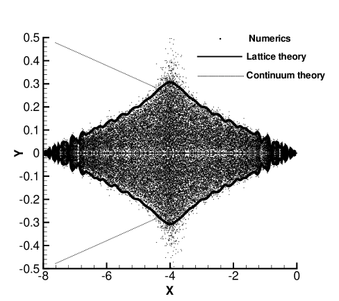
FIG. 4.: Distribution of eigenvalues in the complex plane (dots) and calculated boundary to $\rho(\omega)$ for the lattice theory (full line) and continuum theory (dotted line).

The finite lattice spacing manifests itself in a lower bound to the real part of eigenvalues, and the finite system size studied results in oscillations in the position of the boundary that are apparent in both the numerical and analytical results. A further finite-size effect, clear in the data but not captured in the SCBA we have presented, is that a finite fraction of eigenvalues are purely real: phenomena of this kind in random matrix problems have been analysed in Refs. ([22]) and ([24]).

V Summary

We have described in detail a general technique for calculating average spectral properties of non-Hermitian random operators. We have applied this technique to the Fokker-Planck operator that represents particle diffusion in the presence of random advection. In this way we obtain for the first time the eigenvalue distribution of this operator in the complex plane. The approach is formally exact in the weak disorder limit, and numerical tests show that it is remarkably accurate even for moderately strong disorder. Finally, we have inferred the time-dependent effective diffusivity from the ensemble averaged Green’s function, obtaining a novel scaling in its transient behaviour in the strong disorder limit.

A Corrections to SCBA

We demonstrate in this appendix that corrections to the SCBA expression for the self-energy are small in the coupling constant, $\gamma(|\omega|)$, considering for simplicity the case $\Gamma_{1}=\Gamma_{2}\equiv\Gamma$. We compare the SCBA self-energy, $\Sigma_{11}(p)$, with the contribution arising from the diagram illustrated in Fig. (5), which we denote by $\Sigma^{(2)}_{11}(p)$.

FIG. 5.: Leading correction to the SCBA self-energy.

Our goal is to compute the ratio $\Sigma^{(2)}_{11}(p)/\Sigma_{11}(p)$ in the weak disorder limit. We begin by calculating the correction

$$\Sigma^{(2)}_{11}(p)=\Gamma^{2}\int_{0}^{\Lambda}\int_{0}^{\Lambda}d^{d}q_{1}d^{d}q_{2}({\bf{p}}\cdot{\bf{q}}_{2})^{2}\times$$ (A1)

$$G_{22}(q_{1})G_{11}(q_{2})G_{22}({\bf{p}}+{\bf{q}}_{2}-{\bf{q}}_{1})\,.$$ (A2)

First, consider the region of the complex $\omega$ plane in which the Fokker-Planck eigenvalue density, calculated within the SCBA, is zero (all $y$ for $x>0$, and $|y|>y_{B}$ for $x<0$). In that region, for small $\eta$, $G_{ii}(p)\propto\eta$, $\Sigma_{11}(p)\propto\eta$, $\Sigma^{(2)}_{11}(p)\propto\eta^{3}$ and the ratio has the limiting value $\Sigma^{(2)}_{11}(p)/\Sigma_{11}(p)=0$ for $\eta\to 0$. Second, consider the complementary region ($x<0$ and $|y|<y_{B}$). In this region, we use the same approach for evaluating Eq. (A2) as was applied to Eqs. (33) and (35) in Sec. III. Substituting for $G_{ii}(p)$ in terms of $C(p)$, replacing $C(p)$ with $I(\omega)\delta(p^{2}-q^{2}_{0})$ where $Dq_{0}^{2}+x=0$, and using Eqs. (25) and (43) to obtain $\Sigma_{ii}(p)$ and $I(\omega)$, we find, for $p=q_{0}$ in the limit $\eta\to 0$

$$\Sigma^{(2)}_{11}(p)=\frac{(y_{B}^{2}-y^{2})^{3/2}}{\overline{\Gamma}q_{0}^{2}}f$$ (A3)

where $f$ is an angular average over directions of ${\bf{q}}_{1},{\bf{q}}_{2}$, represented by the unit vectors $\hat{n_{1}}$ and $\hat{n_{2}}$

$$f\equiv\langle(\hat{n_{1}}\cdot\hat{n_{2}})^{2}\delta([\hat{n}+\hat{n_{2}}-\hat{n_{1}}]^{2}-1)\rangle_{\hat{n_{1}}\hat{n_{2}}}={\cal O}(1)\,.$$ (A4)

Thus, for $|y|<y_{B}$, corrections to the SCBA have relative size

$$\frac{\Sigma^{(2)}_{11}(p)}{|\Sigma_{11}(p)|}=\frac{y_{B}^{2}-y^{2}}{\overline{\Gamma}q_{0}^{2}}f\sim\gamma(x)\,,$$ (A5)

and, as advertised, are small at weak disorder.

B Study of discretized problem

On a lattice, with site labels $\alpha$, $\beta$ in arbitrary dimension, the advection part of the Fokker-Planck operator, $-\nabla\cdot{\bf{V}}$, is represented by a matrix with elements

$$A_{\alpha\beta} = -\frac{1}{2}u_{\alpha\beta}$$ (B1)

for $\alpha$, $\beta$ nearest neighbor sites. It satisfies $A_{\alpha\beta}=-A_{\beta\alpha}$ and has diagonal elements

$$A_{\alpha\alpha}=-\frac{1}{2}\sum_{\beta}u_{\alpha\beta}$$ (B2)

so that $\sum_{\alpha}A(\alpha,\beta)=0$, as required for conservation of particle density. Other elements are zero. We take $A_{\alpha\beta}$ to be Gaussian distributed with zero mean, and variance

$$\left<A_{\alpha\beta}A_{\alpha\beta}\right> = \Gamma\pi^{2}\hskip 14.22636pt\left<A_{\alpha\beta}A_{\beta\alpha}\right>=-\Gamma\pi^{2}$$ (B3)

$$\left<A_{\alpha\alpha}A_{\alpha\beta}\right> = \Gamma\pi^{2}\hskip 14.22636pt\left<A_{\alpha\alpha}A_{\beta\alpha}\right>=-\Gamma\pi^{2}$$ (B4)

$$\left<A_{\alpha\alpha}^{2}\right> = 4\Gamma\pi^{2}\hskip 14.22636pt\left<A_{\alpha\alpha}A_{\beta\beta}\right>=-\Gamma\pi^{2}.$$ (B5)

for $\alpha$, $\beta$ nearest neighbor sites. With the plane-wave basis $\langle{\bf{r}}_{\alpha}|{\bf{k}}\rangle=N^{-1/2}e^{i{\bf{k}}\cdot{\bf{r}}_{\alpha}}$, where ${\bf{r}}_{\alpha}$ is the position coordinate of site $\alpha$ on a lattice with $N$ sites in total, we need $\langle\langle{\bf{q}}|A|{\bf{k}}\rangle\langle{\bf{k}}|A^{T}|{\bf{q}}\rangle\rangle$, which takes the value

$$\langle\left<{\bf{q}}|A|{\bf{k}}\right>\left<{\bf{k}}|A^{T}|{\bf{q}}\right>\rangle=$$ (B9)

$$\frac{1}{N^{2}}\sum_{{\bf{r}}_{1}{\bf{r}}_{2}{\bf{r}}_{3}{\bf{r}}_{4}}\left<A_{{\bf{r}}_{1}{\bf{r}}_{2}}A_{{\bf{r}}_{3}{\bf{r}}_{4}}\right>e^{i{\bf{q}}\cdot({\bf{r}}_{1}-{\bf{r}}_{3})+i{\bf{k}}\cdot({\bf{r}}_{4}-{\bf{r}}_{2})}$$

$$=\frac{4\pi^{2}\Gamma}{N}[(1-\cos{q_{x}})(1+\cos{k_{x}})+$$

$$(1-\cos{q_{y}})(1+\cos{k_{y}})]\,.$$

Similarly,

$$\langle\left<{\bf{q}}|A|{\bf{k}}\right>\left<{\bf{k}}|A|{\bf{q}}\right>\rangle=$$ (B11)

$$-\frac{(2\pi)^{2}\Gamma}{N}\left[\sin(k_{x})\sin(q_{x})+\sin(k_{y})\sin(q_{y})\right]\,.$$

Repeating the style of calculation described in Sec. III, we find that the support of the eigenvalue density of the discretized Fokker-Planck operator has a boundary determined by

$$\frac{(2\pi)^{2}\Gamma}{N}\sum_{q_{x},q_{y}}\frac{(1+\cos{q_{x}})(2-\cos{q_{x}}-\cos{q_{y}})}{|\omega+2D[2-\cos{q_{x}}-\cos{q_{y}}]|^{2}}=1\,.$$ (B12)

In the continuum limit we recover the result

$$\Gamma\int_{0}^{\Lambda}d^{2}q\frac{q^{2}}{|\omega+Dq^{2}|^{2}}=1\,,$$ (B13)

and hence Eq. (48).

REFERENCES

- [1] M. B. Isichenko, Rev. Mod. Phys. 64, 961 (1992).
- [2] G. I. Taylor, Proc. London Math. Soc. 20, 196 (1921).
- [3] L. F. Richardson, Proc. R. Soc. London Ser. A 110, 709 (1926).
- [4] G. K. Batchelor, Auts. J. Sci. Res. 2, 437 (1949), Proc. Camb. Philos. Soc. 48, 345 (1952).
- [5] R. H. Kraichnan, Phys. Fluids 11, 945 (1968), Phys. Rev. Lett. 72, 1016 (1994), K. Gawedzki and A. Kupiainen, Phys. Rev. Lett. 75, 3834 (1995), M. Chertkov, G. Falkovich, I. Kolokolov, and V. Lebedev, Phys. Rev. E. 52, 4924 (1995).
- [6] Ia. Sinai, in Proceedings of the Berlin Conference in Mathematical problems in theoretical Physics, edited by R. Schrader et. al. (Springer, Berlin, 1982), p12.
- [7] D. S. Fisher, Phys. Rev. A 30, 960 (1984); D. S. Fisher, Z. Qiu, S. J. Shenker, and S. H. Shenker, ibid., 3841 (1985).
- [8] J. A. Aronovitz and D. R. Nelson, Phys. Rev. A 30, 1948 (1984).
- [9] V. E. Kravtsov, I. V. Lerner, and V. I. Yudson, J. Phys. A 18, L703 1985); Zh. Eksp. Teor. Fiz. 91, 569 (1996) [Sov. Phys. JETP 64, 336 (1986); Phys. Lett. A119, 203 (1986); I. V. Lerner, Nucl. Phys. A 560, 274 (1993).
- [10] M. W. Deem and D. Chandler, J. Stat. Phys. 76, 911 (1994); M. W. Deem, Phys. Rev. E 51, 4319 (1995).
- [11] S. Alexandar, J. Bernasconi, W. R. Schneider, and R. Orbach, Rev. Mod. Phys. 53, 175 (1981).
- [12] J. P. Bouchaud and A. Georges, Phys. Rep. 195, 127 (1990).
- [13] M. Avellaneda and A. J. Majda, Phys. Rev. Lett. 62, 753 (1989), Commun. Math. Phys. 131, 381 (1990), ibid, 138, 339 (1991).
- [14] A. Fannjiang and G. C. Papanicolaou, Prob. Theo. Relat. Fields 105, 279 (1996), J. Stat. Phys. 88, 1033 (1997).
- [15] D. W. Strook and S. R. S. Varadhan, Multidimensional Diffusion Process (Springer, Berlin, 1963).
- [16] H. Risken, The Fokker-Planck Equation (Spring-Verlag, Berlin and Heidelberg, 1989).
- [17] E. Tosatti, M. Zannetti, and L. Pietronero, Z. Phys. B73, 161 (1988).
- [18] J. Miller and Z. J. Wang, Phys. Rev. Lett. 76, 1461 (1996).
- [19] J. Ginibre, J. Math. Phys. 6, 440 (1965).
- [20] V. L. Girko, Theory Probab. Its Appl. (USSR) 29, 694 (1985).
- [21] H. J. Sommers, A. Crisanti, H. Sompolinsky, and Y. Stein, Phys. Rev. Lett. 60, 1895 (1988).
- [22] N. Lehmann and H. J. Sommers, Phys. Rev. Lett. 67, 941 (1991).
- [23] J. Feinberg and A. Zee, Nucl. Phys. B 504, 579 (1997).
- [24] K. B. Efetov, Phys. Rev. Lett. 79, 491 (1997); Phys. Rev. B 56, 9630 (1997).
- [25] J. T. Chalker and Z. J. Wang, Phys. Rev. Lett. 79, 1797 (1997).
- [26] R. A. Janik, M. A. Nowak, G. Papp, and I. Zahed, Phys. Rev. E. 4100 (1997); R. A. Janik, M. A. Nowak, G. Papp, J. Wambach, and I. Zahed, Nucl. Phys. B 501, 603 (1997).
- [27] N. Hatano and D. R. Nelson, Phys. Rev. Lett. 77, 570 (1996); Phys. Rev. B56, 8651 (1997).
- [28] A. V. Izyumov and B. D. Simons, cond-mat/9811260.
- [29] C. Mudry, B. D. Simons, and A. Altland, Phys. Rev. Lett. 80, 4257 (1998).
- [30] See, for example: A. A. Abrikosov, L. P. Gorkov, and I. E. Dzyaloshinski, Methods of Quantum Field Theory in Statistical Physics (Dover, New York, 1975).
- [31] In this paper, we use the more symmetric form in preference to our previous convention, [25].