Thin superconducting disk with $B$-dependent $J_{c}$ : Flux and current distributions

Abstract

The critical state in a superconducting thin circular disk with an arbitrary magnetic field dependence of the critical sheet current, $J_{c}(B)$, is analyzed. With an applied field $B_{a}$ perpendicular to the disk, a set of coupled integral equations for the flux and current distributions is derived. The equations are solved numerically, and flux and current profiles are presented graphically for several commonly used $J_{c}(B)$ dependences. It is shown that for small $B_{a}$ the flux penetration depth can be described by an effective Bean model with a renormalized $J_{c}$ entering the leading term. We argue that these results are qualitatively correct for thin superconductors of any shape. The results contrast the parallel geometry behavior, where at small $B_{a}$ the $B$-dependence of the critical current can be ignored.

I Introduction

The critical state model (CSM) is widely accepted to be a powerful tool in the analysis of magnetic properties of type-II superconductors. For decades there have been numerous theoretical works devoted to CSM calculations in the parallel geometry, i. e., a long sample placed in parallel applied magnetic field, $B_{a}$. More recently, much attention has also been paid to the CSM analysis of thin samples in perpendicular magnetic fields. For this so-called perpendicular geometry explicit analytical expressions for flux and current distributions have been obtained for a long thin strip [1, 2] and thin circular disk[3, 4, 5, 6] assuming a constant critical current (the Bean model).

From experiments, however, it is well known that the critical current density $j_{c}$ usually depends strongly on the local flux density $B$. This dependence often hinders a precise interpretation of various measured quantities such as magnetization, complex ac susceptibility,[7, 8] and surface impedance.[9] It is therefore essential to extend the CSM analysis to account for a $B$-dependence of $j_{c}$.

In the parallel geometry extensive work has already been carried out, and exact results for the flux density profiles and magnetization,[10, 11, 12, 13], as well as ac losses[10, 11] have been obtained for different $j_{c}(B)$-dependences. In the perpendicular geometry the magnetic behavior is known to be qualitatively different. In particular, due to a strong demagnetization, the field tends to diverge at the sample edges, and the flux penetration depth and ac losses follow different power laws in $B_{a}$ for small $B_{a}$.[1, 2] Unfortunately, the theoretical treatment of the perpendicular geometry is very complicated, and we are not aware of any explicit expressions obtained for the CSM with a $B$-dependent $j_{c}$. However, it is possible to derive integral equations relating the flux and current distributions.[3] Such equations have so far been obtained and solved numerically only for the case of a long thin strip.[14, 15]

In this paper, we derive a CSM solution for a thin circular disk characterized by an arbitrary $j_{c}(B)$. The solution is presented as a set of integral equations which we solve numerically. In this way we obtain the field and current density distributions in various magnetized states. We present results for several commonly used functions $j_{c}(B)$. A special attention is paid to the low-field asymptotic behavior.

The paper is organized as follows. In Sec. II the basic equations for the disk problem are derived. We consider here all states during a complete cycle of the applied field, including the virgin branch. Sec. III contains our numerical results for flux and current distributions as well as for the flux front position. A discussion of the results is presented. Finally, Sec. IV presents the conclusions.

II Basic equations

Consider a thin superconducting disk of radius $R$ and thickness $d$, where $d\ll R$, see Fig. 1. We assume either that $d\geq\lambda$, where $\lambda$ is the London penetration depth, or, if $d<\lambda$, that $\lambda^{2}/d\ll R$. In the latter case the quantity $\lambda^{2}/d$ plays a role of two-dimensional penetration depth. [19] We put the origin of the reference frame at the disk center and direct the $z$-axis perpendicularly to the disk plane. The external magnetic field ${\bf B}_{a}$ is applied along the $z$-axis, the $z$-component of the field in the plane $z=0$ being denoted as $B$. The current flows in the azimuthal direction, with a sheet current denoted as $J(r)=\int_{-d/2}^{d/2}j(r,z)\,dz$, where $j$ is the current density.

To obtain expressions for the current and flux distribution we follow a procedure originally suggested in Ref. [3] and then generalized in Ref. [14] for the case of $B$-dependent $J_{c}$ in a thin strip. The procedure makes use of the Meissner state distributions for $B$ and $J$.

In the Meissner state, where $B=0$ inside the disk, the field outside the disk is given by [3, 4]

$$B_{M}(r,R)=B_{a}+\frac{2B_{a}}{\pi}\left[\frac{R}{\sqrt{r^{2}-R^{2}}}-\arcsin\left(\frac{R}{r}\right)\right],$$ (1)

and the current is distributed according to

$$J_{M}(r,R)=-\frac{4B_{a}}{\pi\,\mu_{0}}\frac{r}{\sqrt{R^{2}-r^{2}}},\quad r<R\ .$$ (2)

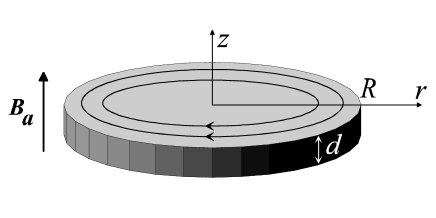
FIG. 1.: Schematic of a thin circular disk in a perpendicular applied field. The current flows in the azimuthal direction.

A Increasing field

We begin with a situation where the external field $B_{a}$ is applied to a zero-field-cooled disk. The disk then consists of an inner flux-free region, $r\leq a$ , and of an outer region, $a<r\leq R$, penetrated by magnetic flux. According to the critical state model, the penetrated part will carry the critical sheet current $J_{c}$ corresponding to the local value of magnetic field,

$$J(r)=-J_{c}[B(r)],\quad a<r<R$$ (3)

Now following Refs. [3, 14], we express the field and current as superpositions of the Meissner-state distributions, (1) and (2), i.e.:

$$B(r) = \int^{\min(r,R)}_{a}\!dr^{\prime}\,B_{M}(r,r^{\prime})\,G(r^{\prime},B_{a})\,.$$ (4)

$$J(r) = \int^{R}_{\max(a,r)}\!dr^{\prime}\,J_{M}(r,r^{\prime})\,G(r^{\prime},B_{a})\,,$$ (5)

where $G(r,B_{a})$ is a weight function. Since $B(r)$ and $B_{M}(r,R)\rightarrow B_{a}$ at $r\rightarrow\infty$ we have the normalization condition

$$\int_{a}^{R}\!dr\,G(r,B_{a})=1\,.$$ (6)

Substituting Eq. (3) and Eq. (2) into Eq. (5) yields an integral equation for the function $G(r,B_{a})$ which can be inverted to obtain

$$G(r,B_{a})=-\frac{B_{c}}{B_{a}}\frac{d}{dr}\int_{r}^{R}\frac{dr^{\prime}}{\sqrt{r^{\prime 2}-r^{2}}}\frac{J_{c}[B(r^{\prime})]}{J_{c0}},$$ (7)

where

$$B_{c}=\mu_{0}J_{c0}/2\,,\quad J_{c0}\equiv J_{c}(B=0).$$ (8)

Note that due to the similar form of the function $J_{M}(r,R)$ in (2) and the Meissner-state current in the strip case[1, 2] our weight function $G(r,B_{a})$ is also similar to that for a strip, see Ref. [14]

From Eqs. (5) and (7) it then follows that the current distribution in a disk is given by

$$J(r)=\left\{\begin{array}[]{lr}-\displaystyle{\frac{2r}{\pi}\int_{a}^{R}\!\!dr^{\prime}\sqrt{\frac{a^{2}-r^{2}}{r^{\prime 2}-a^{2}}}\,\frac{J_{c}[B(r^{\prime})]}{r^{\prime 2}-r^{2}}},&r<a\\ -J_{c}[B(r)],&\!\!a<r<R\end{array}\right.$$ (9)

This equation is supplemented by the Biot-Savart law, which for a disk reads,[3]

$$B(r)=B_{a}+\frac{\mu_{0}}{2\pi}\int^{R}_{0}F(r,r^{\prime})J(r^{\prime})dr^{\prime}\,.$$ (10)

Here $F(r,r^{\prime})=K(k)/(r+r^{\prime})-E(k)/(r-r^{\prime})$, where $k(r,r^{\prime})=2\sqrt{rr^{\prime}}/(r+r^{\prime})$, while $K$ and $E$ are complete elliptic integrals defined as $E(z)=\int_{0}^{\pi/2}\!\left[1-z^{2}\cos^{2}(x)\right]^{1/2}dx$ and $K(z)=\int_{0}^{\pi/2}\!\left[1-z^{2}\cos^{2}(x)\right]^{-1/2}dx$.

The relation between the flux front location $a$ and applied field $B_{a}$ is obtained by substituting Eq. (7) into Eq. (6), giving

$$B_{a}=B_{c}\int_{a}^{R}\frac{dr^{\prime}}{\sqrt{r^{\prime 2}-a^{2}}}\frac{J_{c}[B(r^{\prime})]}{J_{c0}}.$$ (11)

For a given $B_{a}$ and for a specified $J_{c}(B)$ we need to solve the set of three coupled equations (9)-(11). In the case of $B$-independent $J_{c}$, the Eq. (11) acquires the simple form

$$a/R=1/\cosh(B_{a}/B_{c})\,,$$ (12)

and the Eqs. (9) and (10) lead to the Bean-model results derived in Refs. [4] and [5].

Note that the equations can be significantly simplified at large external field where $a\rightarrow 0$ proportionally to $\exp(-B_{a}/B_{c})$. Then $B(r)$ is determined by the single equation

$$B(r)=B_{a}-\frac{\mu_{0}}{2\pi}\int^{R}_{0}F(r,r^{\prime})J_{c}[B(r^{\prime})]dr^{\prime}\,,$$ (13)

following from Eq. (10).

B Subsequent field descent

Consider now the behavior of the disk as $B_{a}$ is reduced after being first raised to some maximal value $B_{am}$. Let us denote the flux front position, the current density and the field distribution at the maximum field as $a_{m}$, $J_{m}(r)$ and $B_{m}(r)$, respectively. Obviously, $J_{m}(r)$, $B_{m}(r)$, and $a_{m}$ satisfy Eqs. (9)-(11).

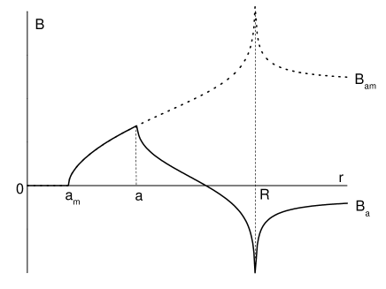
FIG. 2.: Flux density profile during the applied field descent from a maximum value $B_{am}$.

During the field descent from $B_{am}$ the flux density becomes reduced in the outer annular region $a<r<R$, see Fig. 2. The central part of the disk $r<a$ remains frozen in the state with $B_{a}=B_{am}$. Let us specify the field and current distributions in this remagnetized state as

$$B(r)=B_{m}(r)+{\tilde{B}}(r),\quad J(r)=J_{m}(r)+{\tilde{J}}(r),$$ (14)

and derive the relation between ${\tilde{B}}(r)$ and ${\tilde{J}}(r)$. For that one can use a procedure similar to the one described in Sec. II A. The only difference is that in the region $a<r<R$  we now have to use $J(r)=+J_{c}[B(r)]$. In this way we obtain

$${\tilde{J}}(r)=\tilde{J}_{c}(r),\quad\quad\quad a<r<R,$$

where we define

$$\tilde{J}_{c}(r)=J_{c}[B_{m}(r)+{\tilde{B}}(r)]+J_{c}[B_{m}(r)]\,.$$ (15)

Note that the function $\tilde{J}_{c}(r)$ depends on the coordinate only through the field distributions $B_{m}(r)$ and ${\tilde{B}}(r)$. Instead of Eq. (9), the additional current satisfies

$${\tilde{J}}(r)=\left\{\!\begin{array}[]{lr}\displaystyle{\frac{2r}{\pi}\int_{a}^{R}\!dr^{\prime}\ \sqrt{\frac{a^{2}-r^{2}}{r^{\prime 2}-a^{2}}}\,\frac{\tilde{J}_{c}(r^{\prime})}{r^{\prime 2}-r^{2}}},&r<a\\ \tilde{J}_{c}(r),&a<r<R\end{array}\right.$$ (16)

with the complementary equation

$${\tilde{B}}(r)=B_{a}-B_{am}+\frac{\mu_{0}}{2\pi}\int^{R}_{0}F(r,r^{\prime}){\tilde{J}}(r^{\prime})dr^{\prime}\,.$$ (17)

Furthermore, similarly to Eq. (11), we have

$$\frac{B_{a}-B_{am}}{B_{c}}=-\int_{a}^{R}\!\frac{dr}{\sqrt{r^{2}-a^{2}}}\ \frac{\tilde{J}_{c}(r)}{J_{c0}}\ ,$$ (18)

which completes the set of equations describing the remagnetized state. Again, for $B$-independent $J_{c}$ the equations reproduce the Bean-model results [4, 5]

If the field is decreased below $-B_{am}$ the memory of the state at $B_{a}=B_{am}$ is completely erased, and the solution becomes equivalent to the virgin penetration case. If the difference $B_{am}-B_{a}$ is sufficiently large then $a\rightarrow 0$ rapidly, and the critical state $J(r)=J_{c}(r)$ is established throughout the disk. In this case the field descent is described by Eq. (13) with the opposite sign in front of the integral.

We emphasize that the expressions derived here (Sec.II A and B) are readily converted to the long thin strip case. This is due to the similarity of (2) and the expression for the Meissner-current in a strip,

$$J(x)=-\frac{2B_{a}}{\mu_{0}}\frac{x}{\sqrt{w^{2}-x^{2}}},\quad-w<x<w,$$ (19)

where $x$ is the coordinate across the strip. Thus, making in this paper the substitutions

$$r\rightarrow x,\ R\rightarrow w,\ F(r,r^{\prime})\rightarrow\frac{2x^{\prime}}{x^{\prime 2}-x^{2}},\ B_{c}\rightarrow\frac{\mu_{0}J_{c0}}{\pi}$$

one immediately arrives at the set of equations valid for a thin long strip. In that case some of the integrals can be done analytically to yield the expressions obtained in Ref. [14].

A difference between the derivation in Ref. [14] and the present one is that for decreasing fields we calculate only the additional field ${\tilde{B}}(r)$ rather than the total field $B(r)$. This allows us to use only one weight function (7) to calculate the flux distributions both for increasing and decreasing fields. This simplifies the numerical calculations significantly.

C Numerical procedure

Given the $J_{c}(B)$-dependence, the magnetic behavior is found by solving the derived integral equations (9)-(11) numerically using the following iteration procedure. With $B_{a}$ increasing a flux front position $a$ is first specified, and an initial approximation for $B(r)$, e.g., the Bean model solution, is chosen. At each step the $n$th approximation, $B^{(n)}(r)$, is used to calculate $J^{(n)}(r)$ from Eq. (9) and $B_{a}^{(n)}$ from Eq. (11). They are then substituted into Eq. (10) yielding the next approximation, $B^{(n+1)}(r)$. The iterations are stopped when $\left(R^{-1}\int dr\,\left[B^{(n+1)}(r)-B^{(n)}(r)\right]^{2}\right)^{1/2}\leq 10^{-6}B_{c}$. With $B_{a}$ decreasing, the same procedure is used to find first $J_{m}(r)$, $B_{m}(r)$, $B_{am}$ for a given $a_{m}$. Then, Eqs. (16)-(18) are solved for a fixed $a$ yielding the functions ${\tilde{B}}(r)$ and ${\tilde{J}}(r)$ and also the applied field $B_{a}$.

III Flux and current distribution

A General features

In the numerical calculations we used the following dependences $J_{c}(B)$,

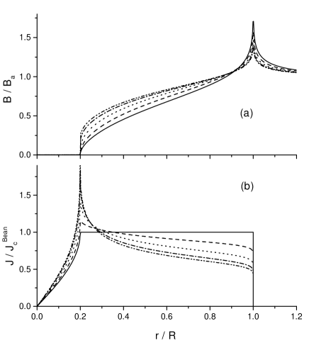
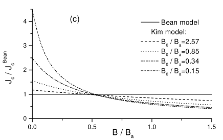
FIG. 3.: Flux density (a) and current (b) profiles for flux penetration into a virgin state. Solid lines are calculated for the Bean model, while other ones represent the Kim model, Eq. (20), with different $J_{c0}$ and $B_{0}$. These parameters are chosen so that the flux front position $a=0.2R$ and applied field $B_{a}$ are the same for all the profiles. The corresponding $J_{c}(B)$-dependences are shown in the panel (c). The current is normalized to the Bean model critical current $J_{c}^{\rm Bean}$.

$$J_{c} = J_{c0}/(1+|B|/B_{0})\quad\quad\ \text{(Kim model),}$$ (20)

$$J_{c} = J_{c0}\,\exp(-|B|/B_{0})\qquad\text{(exponential model).}$$ (21)

Shown in Fig. 3 (a,b) are the field and current distributions for increasing field with $a/R=0.2$ for the Kim model with different parameters $J_{c0}$ and $B_{0}$. They are chosen in a way to keep the position $a$ fixed for all the curves for a given value of $B_{a}$. This allows us to follow the variations in the profile shape as the $B$-dependence of $J_{c}$ changes. The chosen parameters $J_{c0}$ and $B_{0}$ correspond to the set of $J_{c}(B)$-curves shown in Fig. 3 (c). The Bean model results are also plotted in Fig. 3.

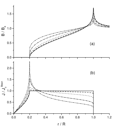
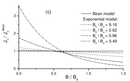
FIG. 4.: Graphs similar to Fig. 3, but here for the exponential model, Eq. (21).

Several major deviations between the Kim and the Bean model can be noticed. In the Kim model we see that (i) the current $J(r)$ is not uniform at $a<r<R$ – it is minimal at the disk edge where $|B|$ is maximal; (ii) the current has a cusp-like maximum at $r=a$ since the magnetic field vanishes at this point with infinite derivative; (iii) compared to the Bean model, the $B(r)$ profiles are steeper near the flux front, whereas the peaks at the edges are less sharp.

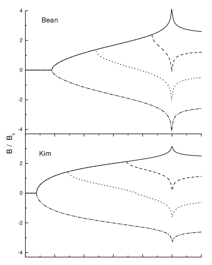
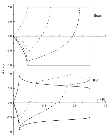
FIG. 5.: Flux density and current profiles for decreasing $B_{a}$. The graphs show the Kim model with $B_{0}/B_{c}=3$ and the Bean model for $B_{a}=B_{am}=2.4B_{c}$ (solid), $B_{a}=1.3B_{c}$ (dashed), $B_{a}=1.3B_{c}$ (dotted), and $B_{a}=-2.4B_{c}$ (dash-dotted).

Qualitatively similar results are obtained for the exponential model, see Fig. 4. Also here, by changing the model parameters one can produce a variety of flux and current profiles which are quite different from the Bean model predictions. When comparing the Kim and exponential model, however, it turns out to be very difficult to find clear distinctions.

During field descent the $B$- and $J$-profiles become more complicated. For brevity we show only profiles for the Kim model with $B_{0}/B_{c}=3$ and for the Bean model at different values of $B_{a}$, see Fig. 5. Again, the Kim model gives a non-uniform current density at $r>a$. Contrary to the increasing-field states, the current density can now either decrease, or increase towards the edge depending on $B_{a}$.

Figure 6 shows profiles for fully-penetrated decreasing-field state. In the Bean model the current remains constant, while the profile of the flux distribution is fixed, although shifted according to the applied field. In contrast, the Kim-model profiles are strongly dependent on $B_{a}$. There is a peak in the current profile and an enhanced gradient of $B(r)$ near the point where $B=0$.

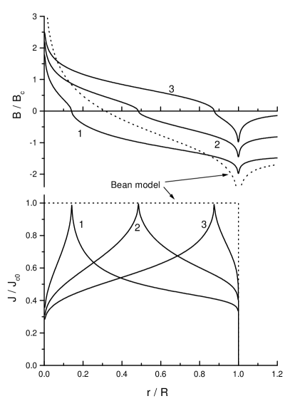
FIG. 6.: Flux and current density profiles during field descent after first increasing $B_{a}$ to a very large $B_{am}$. It is assumed that critical state is established throughout the disk. Solid lines show results for the Kim model with $B_{0}=B_{c}$ and $B_{a}/B_{c}=-1.4$ (curve 1), $B_{a}/B_{c}=-0.7$ (curve 2), and $B_{a}=0$ (curve 3). The dotted lines show the Bean model profiles, their shape being independent of $B_{a}$. In contrast, the shape of the Kim model profiles depends strongly on $B_{a}$.

B Flux penetration depth

To analyze quantitatively the role of a $B$-dependent $J_{c}$ let us consider the position of the flux front during increasing field. A circle with radius $a$ then limits the Meissner region $B=0$, and is also the location of maximum gradient in $B$. These features can be measured directly in experiments on visualization of magnetic flux distribution, e. g., magneto-optical imaging.[20]

Let us first recall the CSM expression for the flux front location in a long circular cylinder in a parallel field [13],

$$\frac{a}{R}=1-\frac{1}{\mu_{0}R}\int_{0}^{B_{a}}\!\frac{dB}{j_{c}(B)}\,.$$ (22)

At small applied fields, $B_{a}$, it can be expanded as

$$\frac{a}{R}\approx 1-\frac{B_{a}}{B_{c}}+\frac{\mu_{0}R}{2}\,j_{c}^{\prime}(0)\,\left(\frac{B_{a}}{B_{c}}\right)^{2}\,,$$ (23)

where for a cylinder $B_{c}\equiv\mu_{0}j_{c0}R$. Note that the $B$-dependence of $j_{c}$ enters the expansion first in the second-order term. Consequently, for a long cylinder the low-field behavior of $a$ is well described by the Bean model where the penetration depth increases linearly with the applied field.

For a thin disk, the penetration of flux proceeds differently. In the Bean model the location of the flux front, Eq. (12), is for small $B_{a}$ given by

$$a/R\approx 1-(1/2)\,(B_{a}/B_{c})^{2}\,.$$ (24)

For an arbitrary $B$-dependence of $J_{c}$ the expression (11) relating $a$ and $B_{a}$ cannot easily be expanded in powers of the ratio $B_{a}/B_{c}$. The physical reason for this is the singular behavior of the magnetic field near the disk edge. There, the local field diverges at any finite $B_{a}$, and an expansion of $J_{c}(B)$ in powers of $B$ is not everywhere convergent. To clarify the behavior of the flux front we have therefore performed numerical calculations of the dependences $a(B_{a},B_{0})$. Shown in Fig. 7 are the results for the Kim (upper panel) and the exponential (lower panel) models. Note that the limit of large $B_{0}$ represents the Bean model.

For small $B_{a}$ all the models seem to yield a parabolic relation between the penetration depth and the applied field. This is illustrated in more detail in Fig. 8, where all the graphs in the log-log plot have a slope of 2 in the low-field region. We therefore conjecture that any $B$-dependence of $J_{c}$ leads to the same quadratic law (24) as for the Bean model, although with different coefficients in front of $(B_{a}/B_{c})^{2}$.

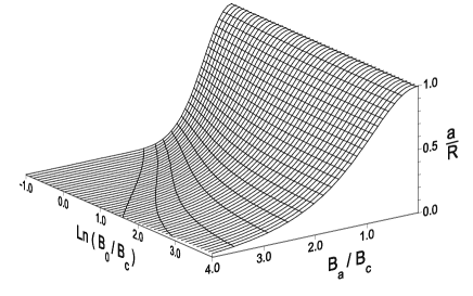
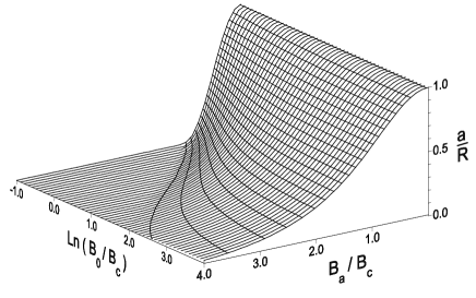
FIG. 7.: Flux front location $a$ as a function of increasing applied field, $B_{a}$, and the charcteristic field, $B_{0}$. The calculated results are presented for the Kim model (upper panel), Eq. (20), and for the exponential model (lower panel), Eq. (21).

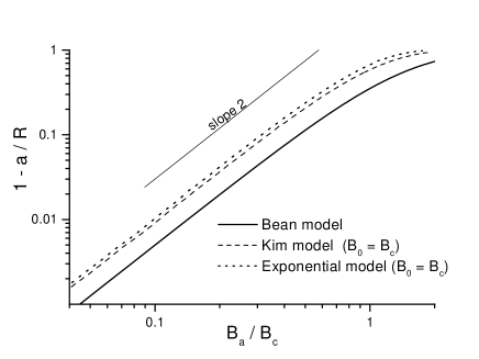
FIG. 8.: Reduced flux penetration depth, $1-a/R$, in the virgin flux-penetrated state versus the applied field, $B_{a}$. For all three models the dependences have quadratic asymptotic behavior at low fields.

The overall behavior of the penetration depth can be fitted well by the full form Eq. (12), provided one makes the substitution $B_{c}\rightarrow B_{c}^{\text{eff}}$, i.e.,

$$a/R=1/\cosh(B_{a}/B_{c}^{\text{eff}})\ .$$ (25)

We find that the effective $B_{c}$ satisfies the relation

$$\frac{B_{c}^{\text{eff}}}{B_{c}}=1-\alpha\,\frac{B_{c}}{B_{0}}\,,$$ (26)

if the ratio $B_{0}/B_{c}$ is of the order 1, or larger. Here $\alpha=0.42$ for the exponential model, and $\alpha=0.36$ for the Kim model. The same relations (25) and (26) are found to hold true for a long thin strip with $\alpha=0.60$ and 0.51 for the exponential and the Kim model, respectively.

We believe that for many purposes a Bean-model description with an effective critical current is appropriate for thin samples of any shape, both in applied field and under transport current. Indeed, strong demagnetization effects always lead to a divergence of magnetic field at the sample edge. This implies that in the sample there is always present a wide range of $B$ values up to infinity. As a result, the sample behavior is determined by the whole $J_{c}(B)$-dependence. In particular, the value $J_{c}(0)$ is not governing the magnetic behavior of thin samples, even when the applied field is very small.[16]

IV Conclusion

A set of integral equations for the magnetic flux and current distributions in a thin disk placed in a perpendicular applied field is derived within the critical state model. The solution is valid for any field-dependent critical current, $J_{c}(B)$. By solving these equations numerically it is demonstrated that both the flux density and current profiles are sensitive to the $J_{c}(B)$-dependence. In particular, compared to the Bean model, the $B(r)$-profiles are steeper near the flux front, whereas the peaks at the edges are less sharp.

Since the local magnetic field at the disk edge is divergent for any value of the applied field, $B_{a}$, a field dependence of $J_{c}$ affects the flux distribution even in the limit of low $B_{a}$. Our numerical calculations show that the flux penetration depth at small fields has the same quadratic dependence on $B_{a}$ as for the Bean model, however with different coefficient. The overall behavior of the flux penetration depth is well described by the Bean model expression with an effective value of the critical current. These results are believed to be qualitatively correct for thin superconductors of any shape. The behavior differs strongly from the case of a long cylinder in a parallel field, where the front position at low $B_{a}$ is not affected by the $B$-dependence of the critical current density.

- [1] E. H. Brandt, and M. Indenbom, Phys. Rev. B 48, 12893 (1993).
- [2] E. Zeldov, J. R. Clem, M. McElfresh, and M. Darwin, Phys. Rev. B 49, 9802 (1994).
- [3] P. N. Mikheenko and Yu. E. Kuzovlev, Physica C 204, 229 (1993).
- [4] J. Zhu, J. Mester, J. Lockhart, and J. Turneaure, Physica C 212, 216 (1993).
- [5] J. R. Clem and A. Sanchez, Phys. Rev. B 50, 9355 (1994).
- [6] Some final expressions obtained in Ref. [3] are not correct, see discussion in Ref. [4].
- [7] F. Gömöry, Supercond. Sci. Technol. 10, 523 (1997).
- [8] B. J. Jönsson, K. V. Rao, S. H. Yun, and U. O. Karlsson, Phys. Rev. B58, 5862 (1998).
- [9] B. A. Willemsen, J. S. Derov, and S. Sridhar, Phys. Rev. B 56, 11989 (1997).
- [10] J. R. Clem, J. Appl. Phys. 50, 3518 (1979).
- [11] M. Forsthuber and G. Hilscher, Phys. Rev. B 45, 7996 (1992).
- [12] M. Xu, D. Shi, R. F. Fox, Phys. Rev. B 42, 10773 (1990).
- [13] T. H. Johansen and H. Bratsberg, J. Appl. Phys. 77, 3945 (1995).
- [14] J. McDonald and J. R. Clem, Phys. Rev. B 53, 8643 (1996).
- [15] An alternative approach to treat the problem is to carry out flux creep simulations.[17, 18] Here the CSM results can be found as a limiting case of a large creep exponent.
- [16] In samples of finite thickness the field divergency at the sample edge is cut off at values of the order of . Thus, the low-field behavior is determined by -dependence at fields less than this value.
- [17] E. H. Brandt, Phys. Rev. B55, 14513 (1997).
- [18] E. H. Brandt, Phys. Rev. B58, 6506 (1998).
- [19] P. G. de Gennes, Superconductivity of Metals and Alloys (Benjamin, New York, 1966).
- [20] Anjali B. Riise, T. H. Johansen, H. Bratsberg, M. R. Koblischka, and Y. Q. Shen, submitted to Phys. Rev. B.; M. R. Koblischka and R. J. Wijngaarden, Supercond. Sci. Technol. 8, 199 (1995).