How to evaluate ground-state landscapes of disordered systems thermodynamical correctly

Abstract

Ground states of three-dimensional EA Ising spin glasses are calculated for sizes up to $14^{3}$ using a combination of a genetic algorithm and cluster-exact approximation. For each realization several independent ground states are obtained. Then, by applying ballistic search and $T=0$ Monte-Carlo simulations, it is ensured that each ground state appears with the same probability. Consequently, the results represent the true $T=0$ thermodynamic behavior. The distribution $P(|q|)$ of overlaps is evaluated. For increasing size the width of $P(|q|)$ and the fraction of the distribution below $q_{0}\equiv 0.5$ converge to zero. This indicates that for the infinite system $P(|q|)$ is a delta function, in contrast to previous results. Thus, the ground-state behavior is dominated by few large clusters of similar ground states.

Keywords (PACS-codes): Spin glasses and other random models (75.10.Nr), Numerical simulation studies (75.40.Mg), General mathematical systems (02.10.Jf).

I Introduction

Recently, a new algorithm for studying the ground-state landscape of finite-dimensional spin glasses [1] was introduced [2]. It could be shown that this method is indeed able to calculate true ground states [3]. The $\pm J$ spin glass (see below) exhibits a ground-state degeneracy, i.e. many different ground states exist for each realization. Results [4] describing the distribution of the ground states depend on the statistical weights of the states which are determined by the algorithm which is used. Usually, different ground states exhibit different weights [5], which is thermodynamically incorrect. Here, a new technique is applied which avoids this problem.

In this work, three-dimensional Edwards-Anderson (EA) $\pm J$ spin glasses are investigated. They consist of $N$ spins $\sigma_{i}=\pm 1$, described by the Hamiltonian

$$H\equiv-\sum_{\langle i,j\rangle}J_{ij}\sigma_{i}\sigma_{j}\quad.$$ (1)

The sum runs over all pairs of nearest neighbors. The spins are placed on a three-dimensional (d=3) cubic lattice of linear size $L$ with periodic boundary conditions in all directions. Systems with quenched disorder of the interactions (bonds) are considered. Their possible values are $J_{ij}=\pm 1$ with equal probability. To reduce the fluctuations, a constraint is imposed, so that $\sum_{\langle i,j\rangle}J_{ij}=0$.

One of the most important questions is whether many pure states exist for realistic spin glasses. For the infinitely ranged Sherrington-Kirkpatrik (SK) Ising spin glass this question was answered positively by the continuous replica-symmetry-breaking mean-field (MF) scheme by Parisi [6]. But also a complete different model is proposed: the Droplet Scaling (DS) theory [7, 8, 9, 10, 11] suggests that only two pure states (related by a global flip) exist and that the most relevant excitations are obtained by reversing large domains of spins (the droplets). From the ground state point of view the existence of many pure states means that two ground states may differ by an arbitrary number of spins. Otherwise two ground states would only differ by the spin orientations in some finite domains, which is always possible in the $\pm J$ model because of the discrete structure of the interaction distribution. A detailed discussion can be found in [12], where the metastate approach [13] is used to thoroughly analyze MF,DS and other intermediate scenarios.

While earlier Monte-Carlo (MC) simulations [14] suffer from small system sizes or equilibration problems [15], recent results of simulations [16] at temperatures just below $T_{c}$ seem to find evidence for the MF picture. In [17], by applying a Migdal-Kadanoff approximation, MF behavior was found for small systems at temperatures slightly below $T_{c}$, where the correlation length exceeds the system size. But by going to lower temperatures or larger systems the DS picture turned out to be more appropriate. Consequently, the analysis of true ground states should clarify the issue. In [18] ground states were calculated using multicanonical MC sampling, but no discrimination between MF and DS could be made because of too small system sizes. Using cluster-exact approximation true ground states [3] were studied and MF behavior was found [4]. But, as mentioned at the beginning, these results suffer from the fact that not all ground states are generated with the same probability [5]. This would indeed be the correct sampling method, since all ground-state configurations have exactly the same energy.

In this work ground states of sizes up to $L=14$ are calculated and a technique is applied, which guarantees that all ground states enter the result with the same weight, i.e. the correct $T=0$ thermodynamical behavior is obtained. It will be shown that the main result changes dramatically: with increasing system size the ground-state behavior is not explained by the MF scenario.

The method presented here is not only useful when the ground state calculation is performed using cluster-exact approximation. Also other methods like simulated annealing or multicanonical simulation do not guarantee a priori that each ground state is calculated with the same probability because always a finite number of steps is used. Thus, the technique presented here has a wide range of applications.

The paper is organized as follows: next a short description of the algorithms is presented. Then the definitions of the observables evaluated here are shown. In the main section the results are presented and finally a summary is given.

II Algorithms

The calculation of ground states for three-dimensional spin glasses belongs to the class of the NP-hard problems [19], i.e. only algorithms with exponentially increasing running time are available. Thus, only small systems can be treated. The basic method used here is the cluster-exact approximation (CEA) technique [2], which is a discrete optimization method designed especially for spin glasses. In combination with a genetic algorithm [20, 21] this method is able to calculate true ground states [3] up to $L=14$. Using this technique one does not encounter ergodicity problems or critical slowing down like when using algorithms which are based on Monte-Carlo methods.

But, as mentioned before, by applying pure genetic CEA, one does not obtain the true thermodynamic distribution of the ground states [5], i.e. not all ground states contribute to physical quantities with the same weight. For small system sizes up to $L=4$ it is possible to avoid the problem by generating all $T=0$ states, i.e. averages can be performed simply by considering each ground-state once. Since the ground state degeneracy increases exponentially with the number $N$ of spins, this is not possible for larger system sizes. Instead one has to choose a subset of all configurations. The following procedure is applied to ensure that all ground states appear with the same probability in this selection:

By performing the ballistic-search (BS) algorithm [22] the ground states are grouped into clusters. All states which are accessible via flipping of free spins, i.e. without changing the energy, are considered to be in the same cluster. It has been shown [22] that the number of clusters defined in this way diverges exponentially for the three-dimensional $\pm J$ spin glass. The sizes of these clusters can be estimated quite accurately using a variant of the BS method [22] even if only few ground states per cluster are available. Then a certain number of ground states is selected from each cluster. This number is proportional to the size of the cluster. It means that each cluster contributes with its proper weight. The selection is done in a manner that many small clusters may contribute as a collection as well; e.g. assume that 100 states are used to represent a cluster consisting of $10^{10}$ ground states, then for a set of 500 clusters of size $10^{7}$ each a total number of 50 states is selected. This is achieved by sorting the clusters in ascending order. The generation of states starts with the smallest cluster. For each cluster the number of states generated is proportional to its size multiplied by a factor $f$. If the number of states grows too large, only a certain fraction $f_{2}$ of the states which have already been selected is kept, the factor is recalculated ($f\leftarrow f*f_{2}$) and the process continues with the next cluster.

The states representing the clusters are generated by $T=0$ Monte-Carlo simulation, i.e. iteratively spins are selected randomly and flipped if they are free. The ground states which have been obtained before are used as initial configurations for the MC simulation. MC is able to reproduce the correct thermodynamic distribution, if the simulation time is long enough. Then, all ground-states within a cluster are visited with the same frequency. Later it will be shown that for the largest size $L=14$ and the largest clusters 100 MC steps per spin are sufficient.

Since each cluster appears with a weight proportional to its size and each ground state within a cluster appears with the same probability, on total each ground state has the same likelihood of being generated. Thus, the correct thermodynamic distribution is obtained.

III Observables

For a fixed realization $J=\{J_{ij}\}$ of the exchange interactions and two replicas $\{\sigma^{\alpha}_{i}\},\{\sigma^{\beta}_{i}\}$, the overlap [6] is defined as

$$q^{\alpha\beta}\equiv\frac{1}{N}\sum_{i}\sigma^{\alpha}_{i}\sigma^{\beta}_{i}\quad.$$ (2)

The ground state of a given realization is characterized by the probability density $P_{J}(q)$. Averaging over the realizations $J$, denoted by $[\,\cdot\,]_{av}$, results in ($Z$ = number of realizations)

$$P(q)\equiv[P_{J}(q)]_{av}=\frac{1}{Z}\sum_{J}P_{J}(q)\quad.$$ (3)

Because no external field is present the densities are symmetric: $P_{J}(q)=P_{J}(-q)$ and $P(q)=P(-q)$. Therefore, only $P(|q|)$ is relevant.

The Droplet model predicts that only two pure states exist, implying that $P(|q|)$ converges to a delta function $P(q)=\delta(q-q_{EA})$ for $L\to\infty$ (we don’t indicate the $L$ dependence by an index), while in the MF picture the density remains nonzero for a range $0\leq q\leq q_{1}$ with a peak at $q_{\max}$ ($0<q_{\max}\leq q_{1}$). Consequently the variance

$$\sigma^{2}(|q|)\equiv\int_{-1}^{1}(\overline{|q|}-|q|)^{2}P(q)dq=\overline{|q|^{2}}-\overline{|q|}^{2}$$ (4)

stays finite for $L\to\infty$ in the MF pictures while $\sigma^{2}(|q|)\sim L^{-y}\to 0$ according the DS approach. The combined average of a quantity $X$ over all ground states and over the disorder is denoted with $\overline{X}$. Here, $y$ is the zero-temperature scaling exponent [7] denoted $\Theta$ in [9, 10].

To characterize the contribution from small overlap values separately, which are due to a complex structure of the energy landscape, the weight $X_{q_{0}}$ of the distribution below a given threshold $q_{0}$ is calculated:

$$X_{q_{0}}\equiv\int_{0}^{q_{0}}P(|q|)\,dq\quad.$$ (5)

The overlap defined in (2) can be applied to measure the distance $d^{\alpha\beta}$ between two states:

$$d^{\alpha\beta}\equiv 0.5(1-q^{\alpha\beta})$$ (6)

with $0\leq d^{\alpha\beta}\leq 1$. For three replicas $\alpha,\beta,\gamma$ the usual triangular inequality reads $d^{\alpha\beta}\leq d^{\alpha\gamma}+d^{\gamma\beta}$. Written in terms of $q$ it reads

$$q^{\alpha\beta}\geq q^{\alpha\gamma}+q^{\gamma\beta}-1\quad.$$ (7)

Another characteristic attributed to the MF scheme is that the state space exhibits ultrametricity. In an ultrametric space [23] the triangular inequality is replaced by a stronger one $d^{\alpha\beta}\leq\max(d^{\alpha\gamma},d^{\gamma\beta})$ or equivalently

$$q^{\alpha\beta}\geq\min(q^{\alpha\gamma},q^{\gamma\beta})\quad.$$ (8)

An example of an ultrametric space is given by the set of leaves of a binary tree: the distance between two leaves is defined by the number of edges on a path between the leaves.

Let $q_{1}\leq q_{2}\leq q_{3}$ be the overlaps $q^{\alpha\beta}$, $q^{\alpha\gamma}$, $q^{\gamma\beta}$ ordered according their sizes. By writing the smallest overlap on the left side in equation (8), one realizes that two of the overlaps must be equal and the third may be larger or the same: $q_{1}=q_{2}\leq q_{3}$. Therefore, for the the difference

$$\delta q\equiv q_{2}-q_{1}$$ (9)

$\delta q=0$ holds. For a finite system ultrametricity may be violated, i.e. $\delta q>0$. If a system becomes more and more ultrametric with growing system size, $\delta q$ should decrease while $L\to\infty$. When evaluating $\delta q$, the influence of the absolute size of the overlaps should be excluded. Thus, the third overlap is fixed: $q_{3}=q_{fix}$. In practice overlap triples are used where $q_{3}\in[q_{fix},q_{fix2}]$ holds. This allows to obtain sufficient statistics. In the next section the distribution $P(\delta q)$ is evaluated. For an ultrametric system this quantity should converge to a Dirac delta function with increasing size $L$ [24].

IV Results

Ground states were generated using genetic CEA for sizes $L\in[3,\ldots,14]$. The number of realizations of the bonds per lattice size ranged from 100 realizations for $L=14$ up to 1000 realizations for $L=3$. One $L=14$ run needs typically 540 CPU-min on an 80MHz PPC601 processor (70 CPU-min for $L=12$, $\ldots$, 0.2 CPU-sec for $L=3$), more details can be found in [3]. Each run resulted in one configuration which was stored, if it exhibited the ground state energy. For the smallest sizes $L=3,4$ all ground states were calculated for each realization by performing up to $10^{4}$ runs. For larger sizes it is not possible to obtain all ground states, because of the exponentially rising degeneracy. For $L=5,6,8$ practically all clusters are obtained using at most $10^{4}$ runs [22], only for about 25% of the $L=8$ realization some small clusters may have been missed.

For $L>8$ not only the number of states but also the number of clusters is too large, consequently $40$ independent runs were made for each realization. For $L=14$ this resulted in an average of $13.8$ states per realization having the lowest energy while for $L=10$ on average $35.3$ states were stored. This seems a rather small number. However, the probability that genetic CEA returns a specific ground state increases (sublinearly) with the size of the cluster the state belongs to [25]. Thus, ground states from small clusters do appear with a small probability. Because the behavior is dominated by the largest clusters, the results shown later on are the same (within error bars) as if all ground states were available. This was tested explicitly for 100 realizations of $L=10$ by doubling the number of runs, i.e. increasing the number of clusters found.

Using this initial set of states for each realization ($L>4$) a second set was produced using the techniques explained before, which ensures that each ground state enters the results with the same weight. The number of states was chosen in a way, that $n_{\max}=100$ states were available for the largest clusters of each realization, i.e. a single cluster smaller than one hundredth of the largest cluster does not contribute to physical quantities, but, as explained before, a collection of many small clusters contributes to the results as well. Finally, it was verified that the results did not change by increasing $n_{\max}$.

The number of MC steps used for generating the states was determined in the following way: a ground state was selected randomly from the largest clusters found for the $L=14$ realizations. 100 independent $T=0$ MC runs of length $n_{MC}$ MC steps were performed starting always from this initial state. For the set of 100 final states the distribution of overlaps was calculated. The whole process was averaged over different realizations. In Fig. 1 the average distribution $P_{c}(q)$ of overlaps is shown for different run lengths $n_{MC}$. It can be seen that by increasing the number of MC steps the ground-state cluster is explored better. By going beyond $n_{MC}=100$ steps $P_{c}(q)$ does not change, indicating that this number of MC steps is sufficient to generate ground states equally distributed within a cluster for $L=14$.

The order parameter selected here for the description of the complex ground state behavior of spin glasses is the total distribution $P(|q|)$ of overlaps. The result for the case where all ground states have the same weight is shown in Fig. 2 for $L=6,10$. The distributions are dominated by a large peak for $q>0.8$. Additionally there is a long tail down to $q=0$, which means that arbitrarily different ground states are possible. So far this is the same result as obtained earlier [4] for the case where the weights of the states are determined by the genetic CEA algorithm. But there is a difference: for the old results the weight of the long tail remains the same for all system sizes. Here for $L=10$ small overlaps are about $3/4$ times less likely than for $L=6$.

To study the finite size dependence of this effect, the variance $\sigma^{2}(|q|)$ of $P(|q|)$ was evaluated as a function of the system size $L$. The result is displayed in Fig. 3. Additionally the datapoints from [4] are given. Obviously, by guaranteeing that every ground state has the same weight, the result changes dramatically. To extrapolate to $L\to\infty$, a fit of the data to $\sigma^{2}_{L}=\sigma^{2}_{\infty}+a_{0}L^{-a_{1}}$ was performed. A value of $\sigma^{2}_{\infty}=-0.01(1)$ ($a_{1}=-0.61(15)$) was obtained, indicating that the width of $P(|q|)$ is zero for the infinite system. Consequently, the MF picture with a continuous breaking of replica symmetry cannot be true for three-dimensional $\pm J$ spin glasses.

In Fig. 4 the behavior of the long tail is studied in more detail. The integrated weight $X_{0.5}(L)$ of all overlaps $q<q_{0}\equiv 0.5$ is shown as a function of the system size. Again a fit is used to extrapolate the behavior of the infinite system. A value of $X_{\infty}=-0.01(2)$ is obtained, confirming the result obtained above.

One might suspect that the results can be explained by the fact that with increasing system size the behavior is dominated more and more by one ground-state cluster. To examine this issue the quantity $Y=1-[\sum_{c}w_{c}^{2}]_{av}$ is calculated, where $w_{c}$ is the relative size of cluster $c$. If really one cluster dominates, $Y$ must vanish with increasing system size $L$. In Fig. 5 $Y$ is shown as a function of $L$ for small system sizes $L\leq 8$, where all ground-state clusters have been obtained. Obviously, $Y$ does not decrease. One reason is that the probability $P(n_{c}=1)$ that a realization exhibits just one ground-state cluster (and its inverse) decreases with growing system size (cf. inset). Consequently, there is no single reason explaining the behavior of $P(|q|)$. Additionally, for the interpretation of Fig.5, one has to take into account that the definition of a cluster, although it is very useful for the evaluation of the ground-state landscape, may have no physical meaning.

By collecting all results one obtains the following description for the distribution of overlaps of the infinite system: It consists of a large delta-peak and a tail down to $q=0$, but the weight of that tail goes to zero. This expression is used to point out that by going to larger sizes small overlaps still occur: the number of arbitrarily different ground states diverges [22]. But the size of the largest clusters, which determine the self overlap leading to the large peak, diverges even faster. The delta-peak is centered around a finite value $q_{EA}$. From further evaluation of the results $q_{EA}=0.90(1)$ was obtained.

Finally, it was tested whether the ground states are ultrametrically organized. In Fig. 6 the distribution $P(\delta q)$ is shown for system sizes $L=4,8,12$. Each realization enters the distribution with the same weight. With increasing system size the distributions get closer to $q=0$, indicating that the systems become more and more ultrametric. The same conclusion can be driven from the evaluation of the average value of $\delta q$ as a function of $L$ (cf. inset). This result is similar to the former calculations [4], where the correct $T=0$ distribution was not obtained. But it should be stressed that ultrametricity is only found within a restricted subset of states (here $q_{3}\approx 0.5$). By performing the thermodynamic limit the weight of all regions of state space restricted in this way disappears, i.e. ultrametricity disappears as well.

V Conclusion

Using genetic cluster-exact approximation the ground-state landscape of three-dimensional $\pm J$ spin glasses is investigated. By applying ballistic search and $T=0$ Monte-Carlo simulation it is guaranteed that each ground state enters the result with the same probability, thus a correct thermodynamic distribution is achieved. This technique also can be successfully combined with other methods which are used to generate several configurations from a degenerate ground-state landscape, e.g. with simulated annealing or multicanonical simulation.

The distribution of overlaps is evaluated. For the infinite system it consists solely of two symmetric delta-peaks. This does not imply that there are only two ground-state clusters remaining. On the contrary, the number of ground state clusters grows exponentially with increasing system size but the ground-state behavior is dominated by a few large similar clusters (and their inverse). Therefore, a distinct impression emerges: a huge number of arbitrarily different ground-state clusters exist, but by going to larger and larger sizes most of them become unimportant. This rules out any (nonstandard) MF picture with continuous breaking of symmetry to be valid in total. Interestingly, the result is compatible with the one step replica-symmetry-breaking scheme which was observed for the p-spin glass [26]. It exhibits a simple distribution of overlaps while many different ground-state clusters are possible. However, further work is needed to determine which of the remaining scenarios really holds for finite-dimensional spin glasses.

Please note that the cluster-interpretation depends on the definition of a cluster. By choosing a dynamic which allows flips of more than one spin at a time, a different definition of energy-barriers is implied and thus another kind of clusters. But it should be stressed that the results presented in this work do not depend on the way a cluster is defined. Any method of sorting the ground states into groups will work that takes the number of ground states selected proportional to the size of the group, and ensures that each state of a group has the same probability of being used for the calculation.

Finally, it should be pointed out that not all results previously obtained using genetic CEA are biased by the disbalance of the ground-state distribution. The main outcomes in [3, 27] are not affected. Additionally, although the old data bases on a wrong distribution, the results in [4] prove that there are arbitrary different clusters present. The reason for $P(|q|)\to\delta(q-q_{EA})$ is that most of them become less important.

VI Acknowledgements

The author thanks T. Aspelmeier, K. Bhattacharya, M. Otto and A. Zippelius for interesting discussions. He is gratefull to A. Zippelius and O. Herbst for critically reading the manuscript. The work was supported by the Graduiertenkolleg “Modellierung und Wissenschaftliches Rechnen in Mathematik und Naturwissenschaften” at the Interdisziplinäres Zentrum für Wissenschaftliches Rechnen in Heidelberg and the Paderborn Center for Parallel Computing by the allocation of computer time. The author obtained financial support from the DFG (Deutsche Forschungs Gemeinschaft) under grant Zi209/6-1.

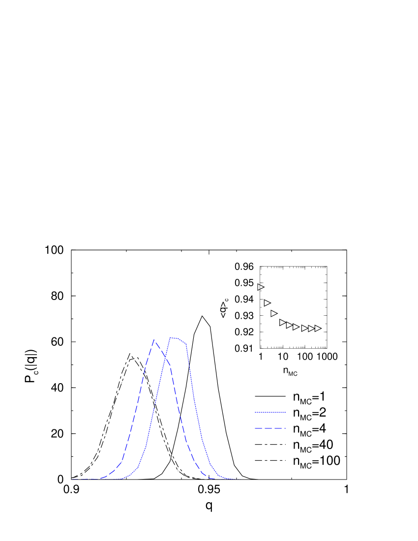
FIG. 1.: Distribution $P_{c}(q)$ of overlaps restricted to a ground-state cluster for different number $n_{MC}$ of MC steps. 100 independent $T=0$ MC runs were performed for the largest clusters found for $L=14$ starting always from the same ground state. By going beyond $n_{MC}=100$ the distribution does not change any more, indicating that 100 MC steps are sufficient to obtain independent ground states within a cluster for $L\leq 14$. The inset shows the mean overlap value as a function of $n_{MC}$.

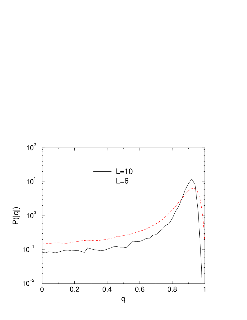
FIG. 2.: Distribution $P(|q|)$ of overlaps for $L=6,10$. Each ground state enters the result with the same probability. The fraction of small overlaps decreases about a factor $3/4$ by going from $L=6$ to $L=10$ (please note the logarithmic scale).

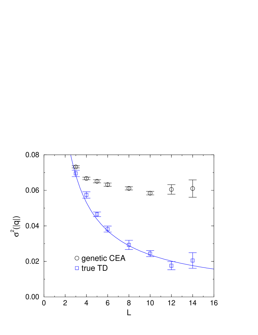
FIG. 3.: Variance $\sigma^{2}(|q|)$ of the distribution of overlaps as a function of linear system size $L$. The upper points show the case were each ground state enters with a weight determined by the genetic CEA algorithm. For the lower points each ground state has the same probability of being included in the calculation. The line represents a fit to $\sigma^{2}_{L}=\sigma^{2}_{\infty}+a_{0}L^{-a_{1}}$. The extrapolation to the infinite system results in $\sigma^{2}_{\infty}=-0.01(1)$. Consequently, the width of distribution of overlaps appears to be zero, i.e. $P(|q|)$ is a delta-function.

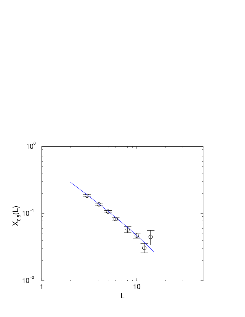
FIG. 4.: Fraction of the distribution of overlaps below $q_{0}\equiv 0.5$ as a function of linear system size $L$. Here the results for the correct thermodynamic average is shown. The line represents a fit to $X_{0.5}(L)=X_{\infty}+x_{0}L^{x_{1}}$. The extrapolation $L\to\infty$ results in $X_{\infty}=-0.01(2)$, i.e. for the infinite systems small values of $|q|$ occur with frequency zero.

FIG. 5.: Cumulant $Y$ describing the distribution of cluster sizes as a function of $L$. For small system sizes $L\leq 8$ almost all ground-state clusters have been obtained. The figure proves that with increasing system size the ground-state landscape is not dominated more and more by one cluster. The inset shows the probability $P(n_{c}=1)$ that a realization exhibits only one ground-state cluster as a function of L.

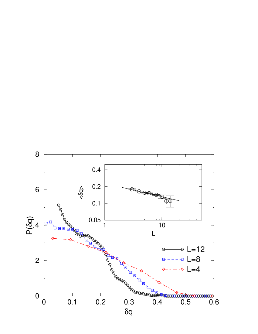
FIG. 6.: Distribution $P(\delta q)$ for different system sizes $L=4,8,12$ where $\delta q=q_{2}-q_{1}$ and $q_{1}\leq q_{2}\leq q_{3}$ are triplets of absolute values of overlaps from independent triplets of ground states. Only triplets with $q_{3}\in[0.5,0.6]$ are used. For an infinite ultrametric system $\delta q=0$ holds. For $L=12$ a running average was used to smooth the data to make the figure more readable. With increasing system size the distributions get closer to $q=0$ indicating the increasing ultrametricity of the ground states. The lines are guides for the eyes only. The inset shows the average value of $\delta q$ as function of system size $L$. The straight line represents the function $\langle\delta q\rangle(L)=0.229\times L^{-0.24}$.

REFERENCES

- [1] For reviews on spin glasses cf.: K. Binder and A.P. Young, Rev. Mod. Phys. 58, 801 (1986); M. Mezard, G. Parisi, M.A. Virasoro, Spin glass theory and beyond, World Scientific, Singapur 1987; K.H. Fisher and J.A. Hertz, Spin Glasses, Cambridge University Press, 1991;
- [2] A.K. Hartmann, Physica A, 224, 480 (1996)
- [3] A.K. Hartmann, Phys. Rev. E 59, 84 (1999)
- [4] A.K. Hartmann, Europhys. Lett. 40, 429 (1997); Europhys. Lett. 44, 249 (1998); Eur. Phys. J. B 8 , 619 (1999)
- [5] A. Sandvic, Europhys. Lett. 45, 745 (1999); A.K. Hartmann, Europhys. Lett. 45, 747 (1999)
- [6] G. Parisi, Phys. Rev. Lett. 43, 1754 (1979); J. Phys. A 13, 1101 (1980); 13, 1887 (1980); 13, L115 (1980); Phys. Rev. Lett. 50, 1946 (1983).
- [7] W.L. McMillan, J. Phys. C 17, 3179 (1984).
- [8] A.J. Bray and M.A. Moore, J. Phys. C 17, L463 (1984); J. Phys. C 18, L699 (1985).
- [9] D.S. Fisher and D.A. Huse, Phys. Rev. Lett. 56, 1601 (1986).
- [10] D.S. Fisher and D.A. Huse, Phys. Rev. B 38, 386 (1988).
- [11] A. Bovier and J. Fröhlich, J. Stat. Phys. 44, 347 (1986).
- [12] C.M. Newmann and D.L. Stein, Phys. Rev. E 55, 5194 (1997)
- [13] C.M. Newman and D.L. Stein, Phys. Rev. Lett. 76, 515 (1996)
- [14] R.N. Bhatt and A.P. Young, Phys. Rev. Lett. 54, 924 (1985); Phys. Rev. B 37, 5606 (1988); A.T. Ogielski and I. Morgenstern, Phys. Rev. Lett. 54, 928 (1985); Phys. Rev. B 32, 7384 (1985); J.D. Reger, R.N. Bhatt and A.P.Young, Phys. Rev. Lett. 64, 1859 (1990) S. Caracciolo, G. Parisi, S. Patarnello and N. Sourlas, J.Phys.(France) 51, 1877 (1990)
- [15] N. Kawashima and N. Ito, J. Phys. Soc. Jpn. 62, 435 (1993)
- [16] E. Marinari, G. Parisi, J. Ruiz-Lorenzo, F. Ritort, Phys. Rev. Lett. 76, 843 (1996).
- [17] M. A. Moore, H. Bokil, and B. Drossel, Phys. Rev. Lett. 81, 4252 (1998)
- [18] B.A. Berg, U.E. Hansmann, T.Celik, Phys. Rev. B 50, 16444 (1994).
- [19] F. Barahona, J. Phys. A 15, 3241 (1982)
- [20] K.F. Pál, Physica A 223, 283 (1996)
- [21] Z. Michalewicz, Genetic Algorithms + Data Structures = Evolution Programs, Springer, Berlin 1992
- [22] A.K. Hartmann, submitted, preprint cond-mat/9902120 and preprint cond-mat/9905128 (1999)
- [23] R. Rammal, G. Toulouse and M.A. Virasoro, Rev. Mod. Phys. 58, 765 (1986)
- [24] R.N. Bhatt and A.P. Young, J. Mag. Mag. Mat. 54-57, 191 (1986)
- [25] A.K. Hartmann, submitted, preprint cond-mat/9904364 (1999)
- [26] D.J. Gross and M. Mezard, Nuclear Physics B 240 [FS12], 431 (1984)
- [27] A.K. Hartmann, Phys. Rev. B 59 , 3617 (1999)