[

Theory of Doped Excitonic Insulators

Abstract

The theory of doped excitonic insulators is reinvestigated in light of recent experiments on hexaborides. For the appropriate valley-degenerate $X_{3},X_{3}^{\prime}$ band structure, “intra-valley” condensation is energetically favored. Ferromagnetism occurs upon doping due to the quenching of kinetic energy at the otherwise direct first-order excitonic insulator–metal transition. The phase diagram includes states of spatially inhomogeneous density and magnetization at low temperatures.

]

Recent dramatic measurements by Fisk et. al.[1] on very lightly-doped divalent hexaborides (${\rm La}_{x}{\rm Ca}_{1-x}{\rm B}_{6}$, ${\rm La}_{x}{\rm Sr}_{1-x}{\rm B}_{6}$, etc.), have revived interest in the physics of excitonic insulators, which are coherent condensates particle-hole excitations that may occur in semi-metals with slightly overlapping or gapped conduction and valence bands. The theory of such excitonic insulators was developed in the 1960’s and 70’s (see Ref. [2] for a review and original references). Band structure calculations predict that ${\rm CaB}_{6}$ and ${\rm SrB}_{6}$ are indeed at the border between very small gap semiconductors and slightly overlapping electron-hole metals (with gap/overlap of $-0.08eV<E_{G}<0.08eV$)[3]. These materials are thus prime candidates for an excitonic instability. The experiments observed ferromagnetism below $T_{c}\sim 600K$ with a small moment maximized around $x=0.005$. Early theoretical work[5] predicted high-temperature ferromagnetism in doped EI’s, and the same connection was recently made for the hexaborides.[4]

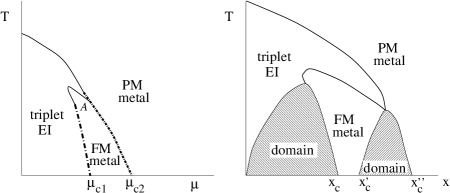
FIG. 1.: Schematic phase diagrams in temperature versus chemical potential $\mu$ and doping $x$ supposing the EI is fully gapped for $x=0$. The thick dashed lines indicate first-order boundaries. If for $x=0$ the system is not fully gapped, a region of triplet EI persists at $T=0$ for small $x$. The order of the phase boundaries near the point $A$ is sensitive to the detailed parameters of the model.

In this letter the theory of EI’s is reinvestigated, taking into account the three-pocket band structure appropriate to the hexaborides. A number of significant errors in the previous work on a two-band model are also corrected. In particular, we find that a first-order transition as chemical potential is varied and a consequent jump in the equilibrium density is crucial in the physics of ferromagnetism (see Fig. 1).

To proceed, we make the crucial physical assumption that the characteristic energy scales of the EI are much smaller than the bandwidth. A natural parameter characterizing this smallness is the ratio of the band gap $E_{G}$ ($E_{G}<0$ for overlapping bands) to the bandwidth $W$. For $|\Gamma|=|E_{G}|/W\ll 1$, the physics is controlled by small momentum-exchange processes. In this limit, the long-range part of the Coulomb potential dominates, and much of the behavior becomes insensitive to the details of the band structure. To make this explicit, we expand the electron field operators $c_{\alpha}^{\vphantom{\dagger}},c_{\alpha}^{\dagger}$ ($\alpha=\uparrow,\downarrow$ is a spin index):

$$c_{\alpha}^{\dagger}({\bf r})=\sum_{ia}\int_{\bf k}^{\Lambda}\phi^{\vphantom{\dagger}}_{i{\bf Q}_{a}+{\bf k}}({\bf r})\psi_{ia\alpha}^{\dagger}({\bf k}).$$ (1)

Here $\phi_{i{\bf k}}({\bf r})$ is a Bloch function at quasi-momentum ${\bf k}$ with $i=1,2$ for valence and conduction states, respectively. The integration ($\int_{\bf k}\equiv\int\!{d^{3}{\bf k}\over{(2\pi)^{3}}}$) is restricted to spheres of radius $\Lambda$ around the regions of band proximity, centered at the three wavevectors ${\bf Q}_{a}=(\pi,0,0),(0,\pi,0),(0,0,\pi)$ (we measure all lengths in units of the lattice spacing). The “flavored” fermion fields (Fourier transformed back to real space) obey $\{\psi_{ia\alpha}^{\vphantom{\dagger}}({\bf r}),\psi_{jb\beta}^{\dagger}({\bf r^{\prime}})\}=\delta_{ij}\delta_{ab}\delta_{\alpha\beta}\delta({\bf r-r^{\prime}}).$ The effective mass approximation is valid for $\Gamma\ll 1$, since then we can take $\Lambda\ll 1$. Thus $H=H_{0}+H_{C}$, with the non-interacting Hamiltonian

$$H_{0}=\sum_{ia\alpha}\int_{\bf k}^{\Lambda}\!\left\{\epsilon_{ia}({\bf k})-\mu\right\}\psi^{\dagger}({\bf k})\psi^{\vphantom{\dagger}}({\bf k}).$$ (2)

Here

$$\epsilon_{ia}({\bf k})=(-1)^{i}\left[{k_{a}^{2}\over{2m^{i}_{\parallel}}}+{(k^{2}-k_{a}^{2})\over{2m^{i}_{\perp}}}-E_{G}\right].$$ (3)

In the Bloch basis, $H_{C}=\overline{H}_{C}+H^{\prime}$, where

$$\overline{H}_{C}=\int_{\bf pqq^{\prime}}^{\Lambda}{2\pi e^{2}\over{p^{2}}}\psi^{\dagger}({\bf q+p})\psi^{\vphantom{\dagger}}({\bf q})\psi^{\dagger}({\bf q^{\prime}-p})\psi^{\vphantom{\dagger}}({\bf q^{\prime}}),$$ (4)

describing the long-range part of the Coulomb interaction, and

$$H^{\prime}\!\!=\!\!\int_{\bf pqq^{\prime}}^{\Lambda}\!\!\!\!G_{ijkl}^{abcd}\psi_{ia\alpha}^{\dagger}({\bf p\!+\!q})\psi_{jb\alpha}^{\vphantom{\dagger}}({\bf p})\psi_{kc\beta}^{\dagger}({\bf p^{\prime}\!-\!q})\psi_{ld\beta}^{\vphantom{\dagger}}({\bf p^{\prime}}).$$ (5)

In the $\Gamma\ll 1$ limit, one finds that $G$ can be approximated as momentum-independent and $O(e^{2}/Q^{2})$, where $Q=O(1)$ is a reciprocal lattice vector. Thus $H^{\prime}\ll\overline{H}_{C}=O(e^{2}/q^{2})$, and can be regarded as a small perturbation.

The approximate “continuum” Hamiltonian $H_{c}=H_{0}+\overline{H}_{C}$ has much higher symmetry than the complete one. Most obviously, $H_{c}$ conserves separately the charge and spin of the electrons of each flavor, which constitutes a $\left[U(2)\right]^{3}$ invariance. Note that $\overline{H}_{C}$ has a much larger $U(12)$ symmetry, which is however strongly broken by the inequivalent dispersion relations in $H_{0}$. As emphasized by Halperin and Rice[2], one may visualize the system at this level as a collection of (flavored) positrons and electrons, which naturally have a strong tendency to bind into “atoms” – excitons. It is thus natural to formally define an “s-wave” excitonic-insulating state by the presence of an off-diagonal expectation value $\langle\psi^{\dagger}_{1a\alpha}({\bf r})\psi^{\vphantom{\dagger}}_{2b\beta}({\bf r})\rangle\neq 0$ for some $a,b,\alpha,\beta$. Clearly, for this order parameter to represent a true symmetry-breaking, there must be no band mixing (at the points ${\bf Q}_{a}$) in the kinetic energy. Mixing is prevented for the hexaborides as the conduction and valence states at $X$ belong to distinct ($X_{3}^{\vphantom{\prime}}$,$X_{3}^{\prime}$) representations of the group of the wavevector. To proceed, we define local pair fields:

$$\Psi_{As}^{\alpha\nu}({\bf r}) = {1\over 2}\psi^{\dagger}({\bf r})T^{A\alpha}\tau^{\nu}\psi^{\vphantom{\dagger}}({\bf r}),$$ (6)

$$\vec{\Psi}_{At}^{\alpha\nu}({\bf r}) = {1\over 2}\psi^{\dagger}({\bf r})T^{A\alpha}\tau^{\nu}\vec{\sigma}\psi^{\vphantom{\dagger}}({\bf r}).$$ (7)

Here and in the rest of the paper we introduce Pauli matrices $\vec{\tau},\vec{\sigma}$ acting in the band and spin spaces, respectively, and $3\times 3$ matrices $T^{A\alpha}$ ($\alpha=1\ldots n_{A}$) acting in the “flavor” space. We also suppress indices wherever possible. The excitonic order parameters are off-diagonal in the band space, and so utilize only the off-diagonal Pauli matrices with $\nu=1,2$. The appropriate $T$’s (which specify irreducible representations of the cubic group – $\Gamma_{1}^{\prime},\Gamma_{3}^{\prime},\Gamma_{5}^{\prime},\Gamma_{4}^{\prime}$ for $A=1,2,3,4$) are U(3) generators. In particular, $T^{11}=I/\sqrt{3}$ and the remainder are expressed in terms of the standard Gell-Mann basis $\{\lambda_{1}\cdots\lambda_{8}\}$: $T^{21}=\lambda_{3}/\sqrt{2}$, $T^{22}=\lambda_{8}/\sqrt{2}$, $T^{31}=\lambda_{1}/\sqrt{2}$, $T^{32}=\lambda_{4}/\sqrt{2}$, $T^{33}=\lambda_{4}/\sqrt{2}$, $T^{41}=\lambda_{2}/\sqrt{2}$, $T^{42}=\lambda_{5}/\sqrt{2}$, $T^{43}=\lambda_{7}/\sqrt{2}$. These satisfy ${\rm Tr}\,T^{A\alpha}T^{B\beta}=\delta^{AB}\delta^{\alpha\beta}$. Due to the separate $U(2)$ invariances for each $ia$ in $\psi_{ia\alpha}$, the order parameters are unified for $H_{c}$ into only two independent multiplets. The first contains the diagonal (in flavor) order parameters with $\Psi_{As}^{\alpha\nu},\vec{\Psi}_{At}^{\alpha\nu}$, with $A=1,2$; the second contains the remaining off-diagonal order parameters with $A=3,4$.

The energetics separation of the above two multiplets is entirely due to the anisotropy in dispersion at the different ${\bf Q}_{a}$ points. Several points suggest that this anisotropy generally favors the diagonal order parameters. A somewhat physical argument is that electrons and holes that can best move together tend to pair more effectively. This suggests that states with similar group velocity at equal momenta (necessary for a zero-momentum condensate) and hence similar dispersion will tend to preferentially bind. Note that anistropies in the interactions also exist, but are much weaker than those in the dispersion.

These heuristic considerations are supported by two concrete calculations. Firstly, consider approach the EI state by reducing $E_{G}>0$ in the band insulator. In this limit, the nature of the condensate is determined by the lowest-energy bound state (which reaches the chemical potential first). It is then necessary to compare the binding energies of electron-hole pairs taken from the same and different ${\bf K}_{a}$. As a caricature of the true band structure, we consider a toy model with $m_{\parallel,\perp}^{1}=m_{\parallel,\perp}^{2}\equiv m_{\parallel,\perp}$ (c.f. Eq. 3). For an electron-hole pair drawn from the same X point, the effective masses match, and the reduced mass in the corresponding anisotropic hydrogen atom problem is $m_{r}=(m_{\parallel}/2,m_{\perp}/2,m_{\perp}/2)$. If the electron and hole are taken from different X points, one obtains instead $m_{r}=(m_{\perp}/2,\tilde{m},\tilde{m})$, with $\tilde{m}=m_{\parallel}m_{\perp}/(m_{\parallel}+m_{\perp})$. Various methods (e.g. variational) can be used to convince oneself that the “diagonal” electron-hole pair is more strongly bound whenever $m_{\parallel}\neq m_{\perp}$. This is particularly clear in the limit $m_{\parallel}\gg m_{\perp}$, in which case the diagonal atom has one very heavy reduced mass component, while all the reduced masses become equal to $m_{\perp}/2$ in the off-diagonal case.

A second argument is provided by diagrammatic techniques which apply deep into the metallic limit when $E_{G}<0$ and Coulomb effects are weak, $e^{2}\sqrt{m}/E_{G}\ll 1$. It is then possible to integrate out modes and further reduce the momentum-space cut-off to a set of spherical shells of width $2\Lambda^{\prime}\ll k_{F}$ around the Fermi surfaces[9]. With the reduced cut-off, fermi-surface renormalization group (RG) arguments[10] or more traditional diagrammatics may be used to show that the only (marginally) relevant two-particle interactions (i.e. which lead to logarithmic instabilities) are valence-conduction “ladder” terms in which a conduction electron is scattered to a valence state at a nearby point on the Fermi surface and vice versa. The most general allowed terms of this type can be written

$$H_{C}=-{1\over 2}\sum_{\nu A\alpha}\int^{\Lambda^{\prime}}\Bigg{[}V^{\nu A\rho}\left|\Psi_{As}^{\alpha\nu}\right|^{2}+V^{\nu A\sigma}\left|\vec{\Psi}_{At}^{\alpha\nu}\right|^{2}\Bigg{]},$$ (8)

where the superscript indicates the spherical shell cut-off, and $\nu=1,2$ sums only over the inter-band $\vec{\tau}$ matrices. Furthermore, to simplify the presentation we have kept only the most relevant s-wave component of each interaction channel; including the full wave-vector dependence is straightforward and leads to no significant modifications. Note that with the sign convention above $V>0$ is an effectively “attractive” interaction. Due to its high symmetry, the continuum interaction $\overline{H}_{C}$ gives identical contributions to all the coupling constants, so $V^{\nu A\rho/\sigma}=V_{0}+\delta V^{\mu A\rho/\sigma}$, with $V_{0}\approx 2\pi e^{2}\ln(k_{F}/\Lambda^{\prime})/k_{F}^{2}$ and

$$\delta V^{\nu A\rho} = \left(G_{ilkj}^{adcb}-2G_{ijkl}^{abcd}\right)\tau_{ji}^{\nu}\tau_{lk}^{\nu}T_{ba}^{A\alpha}T_{dc}^{A\alpha},$$ (9)

$$\delta V^{\nu A\sigma} = G_{ilkj}^{adcb}\tau_{ji}^{\nu}\tau_{lk}^{\nu}T_{ba}^{A\alpha}T_{dc}^{A\alpha}.$$ (10)

Note that the corrections to the singlet interactions, $\delta V^{\nu A\rho}$, have a repulsive “direct” contribution absent in the triplet ($\sigma$) channel, so that the correction terms favor triplet pairing, in agreement with the Hartree-Fock theory of Ref. [2]. Amongst the favored flavor-diagonal representations, there are four possible triplet order parameters, with $A=1,2$, $\mu=1,2$. To decide between them requires an explicit calculation of the Coulomb matrix elements, and hence knowledge of the Bloch states. The simplest wavefunctions consistent with the $X_{3}$,$X_{3}^{\prime}$ symmetries are $\phi_{1}=\sqrt{8}\cos\pi x\sin 2\pi y\sin 2\pi z$, $\phi_{2}=\sqrt{2}\sin\pi x(\cos 2\pi y-\cos 2\pi z)$ for the valence and conduction states at $(\pi,0,0)$, respectively. For these wavefunctions, one finds the most favorable correction occurs to the $A=2$,$\nu=1$ coupling constant, suggesting an EI in the $\Gamma_{3}^{\prime}$ representation. The presence of $\tau^{x}$ pairing indicates broken time-reversal symmetry consistent with a spatially-varying spin density within the unit cell. This result should not be taken as definitive, and might be modified by e.g. including higher harmonics in the Bloch functions. It is crucial to remember, however, that the splittings due to the $\delta V$ terms are only weak perturbations to the continuum contribution from $\overline{H}_{C}$. Thus although a particular EI state is energetically preferred, the other nearly degenerate states can play important roles.

Consider next a mean-field (MF) approach[5, 4]. Following the above reasoning, we include only the diagonal interactions, $V^{\nu A\rho},V^{\nu A\sigma}$, with $\nu=1,2$, $A=1,2$. To allow analytic progress, we also assume the toy model dispersion above and collinear spin polarization of all non-zero order parameters along the $\sigma^{z}$ axis. Define gap functions $\Delta_{a\alpha}^{\nu}={V_{0}\over 2}\langle\psi^{\dagger}_{a\alpha}\tau^{\nu}\psi^{\vphantom{\dagger}}_{a\alpha}\rangle\equiv(\Delta_{as}^{\nu}+\alpha\Delta_{at}^{\nu,z})/2$. The mean-field hamiltonian neglecting $\delta V$ corrections is $H_{MF}=\int_{\bf k}^{\Lambda^{\prime}}{\cal H}_{MF}({\bf k})$ with,

$${\cal H}_{MF}=\sum_{\mu a\alpha}\left\{\psi^{\dagger}_{a\alpha}\left[\epsilon^{a}_{\bf k}\tau^{z}-\mu-\Delta_{a\alpha}^{\mu}\tau^{\mu}\right]\psi_{a\alpha}+{1\over{V_{0}}}\left[\Delta_{a\alpha}^{\mu}\right]^{2}\right\}.$$ (11)

Because ${\cal H}_{MF}$ is a sum of independent terms for different flavors and spin orientations, each such species can be studied separately. To proceed, we note that the hamiltonian for a single species can be mapped to the problem of a BCS superconductor in a Zeeman field. Under the particle/hole transformation $\psi_{2a\alpha}^{\vphantom{\dagger}}\rightarrow\psi_{2a\alpha}^{\dagger}$, $\Delta_{a\alpha}^{1}+i\Delta_{a\alpha}^{2}$ becomes the complex BCS order parameter and $\mu$ the Zeeman field, if valence and conduction states are re-interpreted as up and down spins. This MF theory (MFT) was solved by Larkin and Ovchinnikov[6] and Fulde and Ferrell[7]. For small $\mu$ at low temperatures, a BCS state occurs, with $|\Delta|=\Delta_{0}=2t\exp(-1/N_{0}V_{0})$ at $T=0$, where $t=v_{F}\Lambda^{\prime}$ is an energy cut-off and $N_{0}$ is the density of states at the Fermi level. In the simplest MFT assuming a uniform order parameter, at zero temperature a first order transition occurs at $\mu=\mu_{c}=\Delta_{0}/\sqrt{2}$ directly into the normal state. A more detailed examination shows that an intermediate state with a non-uniform order parameter[6, 7] exists in a narrow region around $\mu=\mu_{c}$, with a first order transition to the BCS state at $\mu=\mu_{c}^{\prime}<\mu_{c}$ and a possibly second order transition to the normal state at $\mu=\mu_{c}^{\prime\prime}>\mu_{c}$. Note that the “non-trivial” solution used in Refs. [4, 5] is actually an unstable and unphysical free energy maximum.

For our purposes, it is sufficient at this stage to consider only the uniform MFT – in any case the non-uniform solution is invalidated by the correction terms soon to be added to Eq. 11. The above analysis indicates that for $\mu=\mu_{c}$, there are two degenerate minima of the single species free energy density

$$f_{a\alpha}=-k_{\rm B}T\int_{\bf k}^{\Lambda^{\prime}}\sum_{\pm}\ln[1+\exp(-\beta\xi_{\pm}({\bf k}))]+{\left[\Delta_{a\alpha}^{\mu}\right]^{2}\over V_{0}}.$$ (12)

Here $\beta=1/(k_{B}T)$ and the quasiparticle energies are $\xi_{\pm}=-\mu\pm\sqrt{\epsilon_{\bf k}^{2}+\Delta^{\mu}\Delta^{\mu}}$. Since the total free energy density is the sum $f_{\rm tot}=\sum_{a\alpha}f_{a\alpha}$, this implies a very large ($2^{2N}$-fold) degeneracy for the full electron-hole system. In particular, the amplitude for each flavor and spin orientation may be chosen independently to equal $0$ or $\Delta_{0}$. While two equal free energy minima occur at any first order transition, this large degeneracy is non-generic.

Additional interactions can split the degeneracy in favor of a ferromagnetic state. The search for symmetry-breaking terms is simplified by the fact that, because the different states have macroscopically different particle occupations, only operators diagonal in flavor and spin have non-vanishing matrix elements in the degenerate subspace. A little examination shows that the dominant perturbations are

$$H^{s}\!=\!\!-\!{1\over 2}\!\sum_{\stackrel{{\scriptstyle A=1,2}}{{\alpha}}}\!\int^{\Lambda^{\prime}}\!\Bigg{[}\delta_{A2}W^{2\rho}\left|\psi^{\dagger}T^{2\alpha}\psi^{\vphantom{\dagger}}\right|^{2}\!\!+\!W^{A\sigma}\!\left|\psi^{\dagger}T^{A\alpha}\vec{\sigma}\psi^{\vphantom{\dagger}}\right|^{2}\Bigg{]}.$$ (13)

A $W^{1\rho}$ term, which represents the long-wavelength Coulomb potential, was neglected, as appropriate for uniform states provided the background charge is taken into account (but see below). Terms involving $\psi^{\dagger}\tau^{z}\psi^{\vphantom{\dagger}}$ were omitted from Eq. 13, as they are important only for band-gap renormalization. Likewise, the $\delta V$ corrections directly couple the $\Delta_{a\alpha}$ order parameters, but are negligibly small: $\delta V\ll W^{A\rho/\sigma}\approx V_{0}$.

Treating the terms in Eq. 13 as perturbations, one finds that to the leading order approximation in which $W^{1\rho}=W^{1\sigma}=W^{2\sigma}$, the lowest energy states for the cubic problem comprise two sets: $8$ with ferromagnetic (but but arbitrarily oriented) polarizations of all flavors (e.g. $\Delta_{a+}=\Delta_{0},\Delta_{a-}=0$), and $12$ with one X-point ungapped, one X-point polarized, and one fully gapped (e.g. $\Delta_{1\pm}=0,\Delta_{2+}=\Delta_{0},\Delta_{2-}=0,\Delta_{3\pm}=\Delta_{0}$). The next order corrections ($\delta W^{1\rho}<\delta W^{2\sigma}<0,\delta W^{1\sigma}>0$) favor the aligned and fully polarized state (note that transverse magnetization $\vec{M}\wedge\vec{\Delta}^{\alpha\mu}_{At}\neq 0$ is never favored).

To understand the behavior with chemical potential in more detail, we expand the MFT and introduce order parameters decoupling the $W^{1\sigma}$ and $W^{2\sigma}$ spin interactions (the $W^{1\rho}$ interaction can also be decoupled, but does not influence the mean-field solution in the physical parameter regime). The extended MFT is obtained by replacing $\mu\rightarrow\mu+\alpha h_{a}$ for flavor,spin $a,\alpha$ and adding the terms

$${\cal H}_{h}={1\over{2J}}(h_{1}^{2}\!+\!h_{2}^{2}\!+\!h_{3}^{2})\!-\!{\delta\over J^{2}}(h_{1}h_{2}\!+\!h_{2}h_{3}\!+\!h_{1}h_{3})$$ (14)

to the original hamiltonian density ${\cal H}_{MF}$. Here $J=\langle 2\pi e^{2}/K^{2}\rangle\gg\delta\sim e^{2}/Q^{2}>0$. It is straightforward to solve the extended MFT for $\delta\ll J$ at zero temperature. One finds a ferromagnetic ground state in the range $\mu_{c1}=\mu_{c}\sqrt{1-2N_{0}J}<\mu<\mu_{c2}=\mu_{c}\sqrt{(1-2N_{0}J)/(1-4N_{0}J)}$, with first order transitions at $\mu_{c1},\mu_{c2}$ (this assumes $\mu_{c2}<\Delta_{0}$). At finite temperature the MFT gives the phase diagram shown in Fig. 1. Note that the above behavior is stable to further perturbations such as the $\delta V$ corrections, except insofar as to stabilize a particular (e.g. $\Gamma_{3}^{\prime}$) triplet state for $\mu<\mu_{c1}$.

A salient feature of the MFT is the first-order nature of the low-temperature boundary of the ferromagnetic phase. Taking into account long-range Coulomb interactions, macroscopic charge neutrality requires that as a function of doping $x$ the system must therefore form an inhomogeneous (i.e. domain or labyrinthine) state for $0<x<x_{c}=6N_{0}\mu_{c1}$, the minimum value in the ferromagnetic phase. It is straightforward to estimate the typical width $\ell$ of ferromagnetic domains (their detailed morphology is much more difficult to determine) which is controlled by a competition between electrostatic energy and surface tension $\sigma\sim N_{0}v_{F}\Delta_{0}$, which set the profile of the electrochemical potential. One finds $\ell\sim\left[\sigma/(e^{2}x^{2}(1-x/x_{c})^{2})\right]^{1/3}$. Note that if $\ell$ becomes of order the “coherence” length $\xi=v_{F}/\Delta_{0}$, this semiclassical analysis is invalid and a microscopic quantum calculation is required. A consequence of the domain state is that the magnetization density is linear in the doping in this region, i.e. $m/x$ is constant (and stays non-zero as $x\rightarrow 0^{+}$). Similar behavior holds for $x_{c}^{\prime}=6N_{0}\mu_{c2}<x<x_{c}^{\prime\prime}=12N_{0}\mu_{c2}$, where a non-uniform mixture of ferromagnetic and normal domains obtains.

Beyond the simplest MFT, it is possible for the system to remain in an unpolarized and uniform excitonic state for very small doping at zero temperature. This can occur only if the undoped excitonic state is itinerant (and therefore gapless). To study the feasibility of this scenario, we have considered an unnested MFT (i.e. with different effective masses for electrons and holes). In this case, an intermediate-coupling excitonic metal phase occurs near $\mu=0$, with a non-vanishing excitonic order parameter but an incompletely gapped Fermi surface. A first order $T=0$ transition to an excitonic ferromagnet remains if the incommensurability is not too large. It is likely that a continuous excitonic paramagnet–ferromagnet transition is prohibited by the singular quasiparticle-mediated interactions, but this issue warrants further investigation.

Many open questions remain. An enormous multitude of collective (pseudo-Goldstone modes of $[U(2)]^{3}$) modes should exist in the $|\Gamma|\ll 1$ limit, mostly with small gaps. There are also a large number of metastable free-energy minima which could lead to substantial hysteresis. Non-trivial topological excitations are also possible. Finally, the role of disorder and possible trapping by dopant ions should be considered. The present analysis provides a framework for systematic studies of these issues, and of the applicability of the excitonic model to the hexaborides.

REFERENCES

• [1] D. P. Young et. al., Nature 397, 412 (1999).
• [2] B. I. Halperin and T. M. Rice, in Solid State Physics, 21, F. Seitz, D. Turnbull, and H. Ehrenreich, eds., Academic Press, New York, 1968.
• [3] S. Massidda et. al., Z. Phys. B 102, 83 (1997); A. Hasegawa and A. Yanase, J. Phys. C 12, 5431 (1979).
• [4] M. E. Zhitomirsky, T. M. Rice and V. I. Anisimov, cond-mat/9904330, unpublished.
• [5] B. A. Volkov et. al., Sov. Phys.-JETP 41, 952 (1976); ibid., 43, 589 (1976).
• [6] A. I. Larkin and Yu. N. Ovchinnikov, Sov. Phys.-JETP 20, 762 (1965).
• [7] P. Fulde and R. A. Ferrell, Phys. Rev. 135, A550 (1964).
• [8] L. Balents, in preparation.
• [9] A proper treatment of the long-range Coulomb interaction in the RG approach will be deferred to Ref.Β [8].
• [10] R. Shankar, Rev. Mod. Phys. 66, 129 (1994).