A novel superconducting glass state in disordered thin films in Clogston limit

Abstract

A theory of mesoscopic fluctuations in disordered thin superconducting films in a parallel magnetic field is developed. At zero temperature and at a sufficiently strong magnetic field, the superconducting state undergoes a phase transition into a state characterized by superfluid densities of random signs, instead of a spin polarized disordered Fermi liquid phase. Consequently, in this regime, random supercurrents are spontaneously created in the ground state of the system, which belongs to the same universality class as the two dimensional $XY$ spin glass. As the magnetic field increases further, mesoscopic pairing states are nucleated in an otherwise homogeneous spin polarized disordered Fermi liquid. The statistics of these pairing states is universal depending on the sheet conductance of the 2D film.

I Introduction

Recent experiments on thin superconducting films in a parallel magnetic field [1] have rekindled interest in this field. If the thickness of the films $d$ is small enough, the orbital effect of the magnetic field can be neglected and the suppression of superconductivity in the film is due to the Zeeman effect [2, 4, 3]. It has been observed that the resistance of such films at low temperatures and high enough magnetic fields exhibits very slow relaxation in time [1]. This behavior is characteristic for spin and superconducting glasses. Below we discuss a possibility that mesoscopic fluctuations of superconducting parameters in disordered films account for such a behavior.

Mesoscopic physics in a noninteracting electron system has been known for a while[5, 6]. The energy spectrum in a mesoscopic sample was shown to exhibit Wigner-Dyson statistics, which is universal, only dependent on the symmetry of the Hamiltonian[7]. The long range level repulsion in the energy spectrum leads to a suppression of fluctuations of levels within an energy band of width $E_{c}=D/L^{2}$(Thouless energy). $L$ is the length of the sample, $D={v_{F}l}/{3}$ is the diffusion constant of the film. $v_{F}$ is the Fermi velocity, $l$ is the elastic mean free path. For an open sample, the fluctuation of number of levels $\delta N$ within the energy band of Thouless energy $E_{c}$ is of order unity,

$$\frac{<(\delta N)^{2}>}{<N>^{2}}=\frac{\beta}{G^{2}}$$ (1)

for a $2D$ film, where the corresponding average number of levels $<N>=L^{2}d\nu_{0}E_{c}=G$, with $\nu_{0}$ being the average density of states in the metal on the Fermi surface. $\beta$ is a factor of order unity depending on the symmetry of the Hamiltonian. $G=k_{F}^{2}dl$, is the dimensionless conductance of the $2D$ normal metal in units of ${e^{2}}/{\hbar}$, $k_{F}$ is Fermi wave length and the brackets $\langle\rangle$ denote averaging over realizations of random potential. Consequently, the transport is governed by UCF (universal conductance fluctuation) theory. The conductance exhibits sample specific fluctuations, with amplitude $e^{2}/\hbar$, independent of the average conductance of the sample[5, 6]. More generally, any physical quantity in a mesoscopic sample consist of an ensemble average part and a sample specific part due to quantum interference.

On the other hand, disordered superconductors have been studied long ago [2]. It was shown that the ground state condensate wave function is homogeneous and the critical temperature remains unchanged in the presence of weak nonmagnetic disorders. To derive the dirty superconductor theory, one has to assume that 1). the effective interaction constant in the Cooperon channel remains the same as in a clean superconductor; 2). the condensate wave function is translationally invariant; 3). the time reversal symmetry is preserved. The first assumption, though is not true in the thin film limit where the Coulomb interaction in Cooperon channel can be greatly enhanced, is valid in the bulk limit[8]. We will assume its validity because it does not affect the result present in this paper as far as the renormalized interaction constant is still negative. The translation invariance is not a generic symmetry of the original Hamiltonian in the presence of disorder and the second assumption is true only after the impurity average is taken in the semiclassical limit. The sample specific quantum interference effect which is of the same origin of Wigner-Dyson statistics was not taken into account. The consequency of such an effect which breaks the translation invariance is one of the subjects of this article.

The most fundamental aspect of Anderson theory for a dirty superconductor is the absence of spontaneous time reversal symmetry breaking; that is, the stability of a BCS state with respect to possible frustrations, even when $l$ is much shorter than the coherence length. This is in contrast to how a ferromagnet responses to impurities: A spin glass phase which does not have a conventional long range order but does have Edward-Anderson type long range order always takes over when impurities are added into the system[9]. This central issue will be addressed in this article, in connection with nodes in the spatial dependence of exchange interactions and the distribution function of the exchange interactions.

Unlike in the noninteracting metal where the mesoscopic physics is relevant only in a finite sample smaller than the dephasing length, in the presence of off-diagonal long range order, it reveals itself in the thermodynamic limit. However, when the elastic mean free path $l$ exceeds the Fermi wave length $\hbar/k_{F}$, mesoscopic fluctuations of various physical parameters of superconductors are smaller than their averages [10, 11, 12, 13]. Thus, it seems that they hardly affect macroscopic observable quantities. It was realized later that there are situations where mesoscopic fluctuations determine macroscopic properties of a superconducting sample. One example is a superconductor in a magnetic field close to the upper critical field $H_{c2}$, where the magnetic field dependence of the superconducting critical temperature is determined by the mesoscopic fluctuations [14]. In general, the mesoscopic effects are not only relevant in a disordered superconductor but also determinant to the global phase rigidity.

In this paper we consider the case, where the magnetic field is parallel to the thin superconducting film and the main contribution to the suppression of superconductivity by the magnetic field is due to Zeeman splitting of electron spin energy levels. We show that at low temperatures $T$ and high enough magnetic fields $H$, parallel to the film, the system exhibits a transition into a state where the local superfluid density $N_{s}({\bf r})$ (which is the ratio between the supercurrent density ${\bf J}_{s}$ and the superfluid velocity ${\bf V}_{s}$) has a random sign. In this case the system belongs to the same universality class as the two-dimensional XY spin glass model with exchange interaction of random signs. We also find that as the magnetic field is decreased from above the critical field, mesoscopic pairing states are nucleated in an otherwise spin polarized disordered Fermi liquid. The characteristic length scale at which pairing takes place increases as the critical field is approached. The statistics of these pairing state is universal depending on the sheet conductance only.

The idea that the superfluid density can be of random signs has a long history [15, 10, 11, 12, 16, 17, 18]. However, in the absence of magnetic fields and at zero temperature in disordered superconductors ($\xi_{0}\gg l\gg{\hbar}/{k_{F}}$) the variance of the superfluid density, averaged over the superconducting coherence length $\xi_{0}=\sqrt{{D}/{\Delta_{0}}}$, turns out to be much smaller than its average [10, 11, 12, 13]

$$\frac{\langle(\delta N_{s})^{2}\rangle}{\langle N_{s}\rangle^{2}}=\frac{1}{G^{2}}\ll 1,$$ (2)

$\Delta_{0}$ is the value of the order parameter at $T,H=0$. Similarity between Eqs.1,2 suggests the intimate relationship between the fluctuations of the superfluid densities and universal Wigner-Dyson statistics. In fact, Eq.2. follows as a consequency of the fluctuation of number of levels within Thouless energy band in a volume of size of the coherence length $\xi_{0}$. As long as $k_{F}l\gg\hbar$, the regions where the superfluid density is negative are rare and do not contribute significantly to macroscopic properties of superconductors. The situation in the presence of a magnetic field parallel to the film is different, because the average superfluid density decays with $H$ faster than its variance. Hence, at high enough magnetic field the amplitude of the mesoscopic fluctuations of $N_{s}({\bf r})$ becomes larger than the average, and the respective probabilities of having positive and negative signs of $N_{s}({\bf r})$ are of the same order even at $k_{F}l/\hbar\gg 1$(See below). This was first pointed out in an early paper by the author[19].

In section 2, we present the qualitative picture of this phenomenon, emphasising on the sensitivity of mesoscopic fluctuations of spin polarization energy to the change of the pair potential. In section 3, we study the mesoscopic fluctuations of the superconducting order parameter near the critical regime and show that there are spontaneously created currents in the ground state. In section 4, we derive the distribution function of the ground state condensate wave function at a magnetic field higher than the critical one. In section 5, we discuss the role of the exchange interaction. In section 6, we discuss the mesoscopic effects in a finite size superconductor. In conclusion, we propose possible experiments to observe these effects and point out a few open questions, including implications on d-wave superconductors.

II Qualitative Picture

A theory of magnetic field induced phase transition which does not take into account mesoscopic fluctuations predicts [20, 21, 2] that at low temperatures the superconductor-normal metal transition, is of first or second order depending on whether the parameter $\Delta_{0}\tau_{so}$ is larger or smaller than unity respectively. Here, $\tau_{so}$ is the spin-orbit relaxation time. The $H$-dependence of the order parameter for the two limiting cases was discussed extensively in[20, 21].

From now on, we restrict ourselves to the limit $\Delta_{0}\tau_{so}\ll 1$, where the theory predicts a second order phase transition between the superconducting state and the normal state. At $T=0$ and within an approximation which neglects mesoscopic effects, the value of the critical magnetic field $H^{0}_{c}$ is the result of the competition between the average superconducting condensation energy density $\langle E_{c}\rangle\sim\nu_{0}\Delta_{0}^{2}$ and the polarization energy of the electron gas in the magnetic field. The average spin polarization energy density of nonsuperconducting electron gas is of order $\langle E_{p}(0)\rangle\sim\nu_{0}(\mu_{B}H)^{2}$. Its relative change in the superconducting state is of order $\langle E_{p}(0)\rangle-\langle E_{p}(\Delta)\rangle\sim\frac{3}{4}\pi\Delta_{0}\tau_{so}\langle E_{p}(0)\rangle\ll\langle E_{p}(0)\rangle$ [22, 23, 24]. As a result we get an expression for the critical magnetic field $H^{0}_{c}=H_{cc}(\Delta_{0}\tau_{so})^{-\frac{1}{2}}\gg H_{cc}$. Here $H_{cc}={\Delta_{0}}/{\mu_{B}}$ is the Chandrasekar-Clogston critical magnetic field of the superconductor-normal metal transition for $\Delta_{0}\tau_{so}\rightarrow\infty$ and $\mu_{B}$ is the Bohr magneton.

Consider the mesoscopic fluctuations of the quantities, discussed above, in a volume whose size is of the order of the coherence length $\xi_{0}$. To calculate the amplitude of mesoscopic fluctuations of the polarization energy $\delta E_{p}$, we use the conventional diagram technique for averaging over realizations of random potentials[25]. By evaluating the diagrams in Fig.2.d (see Appendix A), we have

$$\sqrt{\langle(\delta E_{p})^{2}\rangle}\propto\frac{1}{G}(\Delta_{0}\tau_{so})\langle E_{p}(0)\rangle.$$ (3)

This part of the polarization energy is sensitive to the change of the pair potential($H\sim H_{c}$) just as the quantum interference effect is sensitive to the change of impurity potentials. The $\Delta$-dependent part of the mesoscopic fluctuation of spin polarization energy can be obtained by calculating the diagrams in Fig.2.d,

$$\sqrt{\langle(\delta E_{p}(\delta\Delta)-\delta E_{p}(\Delta=0))^{2}\rangle}\propto\frac{1}{G}(\tau_{so}\Delta_{0})<E_{p}(0)>\frac{\delta\Delta^{2}}{\Delta_{0}^{2}}.$$ (4)

Linear in $\delta\Delta$ term vanishes because a quasiparticle is reflected into a quasi hole when it is scattered by $\delta\Delta$. As a result, the change of mesoscopic fluctuations of the spin polarization energy associated with the change of the pair potential $\delta\Delta$ of order $\Delta(H)$ is given as

$$\sqrt{\langle(\delta E_{p}(\Delta(H))-\delta E_{p}(\Delta=0))^{2}\rangle}\propto\sqrt{\langle(\delta E_{p}(0))^{2}\rangle}\left(\frac{\Delta(H)}{\Delta_{0}}\right)^{2}.$$ (5)

Eq.5 shows that below the critical field, though the average cost of condensation energy and kinetic energy to have a configuration with order parameter equal to zero in some regions are positive, the mesoscopic fluctuations of polarization energy associated with such a configuration are of random signs. Since both the polarization energy and the condensation energy are fluctuating quantities, $\Delta({\bf r})$ should also be spatially fluctuating. Particularly, when $H^{0}_{c}$ is approached, the average cost of energy vanishes, the spatial structure of the order parameter is completely determined by mesoscopic fluctuations of spin polarization energy. One elaborates the following argument to confirm this picture.

Consider a domain of size $L_{D}\gg\xi_{0}$ where the value of $\Delta({\bf r})$ differs from its bulk value by a factor of order unity. An estimate for the energy of such a domain consists of three terms, namely

$$\delta E(\Delta)=\nu_{0}\Delta(H)^{2}d(C_{1}\frac{1}{G}L_{D}\xi_{0}+C_{2}\frac{H_{c}^{0}-H}{H^{0}_{c}}L_{D}^{2}+C_{3}\xi_{0}^{2})$$ (6)

where $C_{1},C_{2},C_{3}$ are factors of order of unity. The first term in Eq.6 corresponds to the $\Delta$-dependence of mesoscopic fluctuations of polarization energy and has a random sign. When estimating this term we have taken into account that regions of size $\xi_{0}$ make independent random contributions into Eq.6. The second and third term are the average condensation energy and surface (gradient) energy of the domain, respectively. It follows from Eq.6 that when $L_{D}\sim\xi(H)=\xi_{0}{\Delta_{0}}/{\langle\Delta(H)\rangle}$, there is an interval of magnetic fields near the critical one

$$H_{c}^{0}-H\sim\frac{H^{0}_{c}}{G^{2}}$$ (7)

where the first term is larger than the second and the third ones. Here $\langle\Delta(H)\rangle=\Delta_{0}\sqrt{(H^{0}_{c}-H)/H^{0}_{c}}$ is the average superconducting order parameter. It means that, in this case the spatial distribution of $\Delta({\bf r})$ is highly inhomogeneous and the amplitude of the spatial fluctuations of $\Delta({\bf r})$ is of order of its average, while the characteristic size of the domains is of order of $L_{D}\sim\xi(H=H_{c}^{0}(1-1/{G^{2}}))\sim\xi_{0}G$. At $H$ far away from $H^{0}_{c}$, the typical mesoscopic fluctuations are smaller than the average contribution and do not change the most probable configuration; they only introduce exponentially small concentrations of defects originating from the statistically rare events.

The second kind of the instability which is intimately connected with this inhomogeneous mesoscopic superconducting state is spontaneous creation of long range current. In other words, the superfluid density, which is the second derivative of the energy with respect to superfluid velocity in this region has a random sign and is no longer positive defined. To see this, one should consider states with finite superfluid velocity ${\bf V}_{s}=\frac{1}{m}(\nabla\chi+{2e}/{c}{\bf A}$), where $\chi({\bf r})$ is the phase of the order parameter, $m$ is the electron mass and ${\bf A}({\bf r})$ is the vector potential, which has a direction parallel to the film and $m$ is the electron mass. If ${\bf V}_{s}({\bf r})$ is of the order of the critical velocity, all three terms in Eq.6 are modified by factors of order of unity when compared with the case ${\bf V}_{s}=0$. The second and the third term in Eq.6 decrease with ${\bf V}_{s}$, while the first term is changed in a random direction. This means that at high enough magnetic fields, states with nonvanishing value of ${\bf V}_{s}({\bf r})$ can have lower energy than the states with ${\bf V}_{s}=0$, and that the system is unstable with respect to the creation of supercurrents flowing in random directions. In this estimate we neglect the energy of the magnetic field associated with ${\bf V}_{s}({\bf r})$ in the thin film limit. Since at each point of the system the possible energy gain associated with finite value of ${\bf V}_{s}({\bf r})$ is independent of the direction of ${\bf V}_{s}$, the ground state of the system is highly degenerate and belongs to the same universality class as $XY$ spin glass with a random sign of the exchange interaction.

In principle, both the spin polarization energy and the condensate energy fluctuate from region to region. Both are related to the density of states, though the condensate energy should be determined by the solution of the self consistent equation. For the above argument to be true, we have to assume that the spin polarization energy and the condensate energy fluctuate independently. The argument can be carried out in a similar fashion even if these two are partially correlated, as far as they are not fully correlated[26]. More serious consideration of the existence of inhomogeneous state is addressed in term of the self consistent equation in the next section.

It is important to mention that even in the case of small magnetic fields in the presence of spin orbit scattering the time reversal symmetry is broken and the electron wave functions are complex. Therefore there are currents in the ground state of the system which have random directions. These currents exist even in normal metals. Diagrammatic calculation leads to an expression for the correlation function of the current density ${\bf J}({\bf r})$ in a normal metal induced by a magnetic field ($|{\bf r}-{\bf r^{\prime}}|\gg{\hbar}/{k_{F}}$) as shown in [19]

$$\langle{\bf J}_{i}({\bf r}){\bf J}_{j}({\bf r^{\prime}})\rangle\approx\delta_{ij}\frac{e^{2}}{\hbar^{4}d^{2}}\tau\tau_{so}(\mu_{B}H)^{4}\delta({\bf r}-{\bf r^{\prime}}).$$ (8)

Here $\tau={l}/{v_{F}}$ is the elastic mean free time. It is important to note, however, that for a given configuration of the scattering potential and at a given value of the external field the spatial distribution of ${\bf J}({\bf r})$ is a unique function. This implies that the currents described by Eq. 8 do not exhibit features which can be associated with superconducting glass states. In other words, at small $H$ the superfluid density of the superconducting state is positive which means that states with nonzero superfluid velocity have larger energy than the ground state. The rare regions, where $N_{s}({\bf r})<0$ and the supercurrents exist in the ground state, are screened effectively due to the Meissner effect. They do not affect significantly the macroscopic behavior of a sample.

III Condensate wave function: $H\leq H_{c}^{0}$

Below, we will be interested in supercurrents much larger than those described by Eq.8. Such currents are spontaneously created at strong enough magnetic fields as a result of the instability associated with the random sign of superfluid density. To evaluate the variance of the superfluid density we consider the Gorkov equation for $\Delta({\bf r})$[25],

$$\Delta({\bf r})=g\int d{\bf r^{\prime}}K({\bf r},{\bf r^{\prime}};H,{\bf A}({\bf r}),\{\Delta({\bf r})\})\Delta({\bf r^{\prime}}),$$ (9)

where $g$ is the dimensionless interaction constant,

$$K({\bf r},{\bf r^{\prime}};H,{\bf A}({\bf r}),\{\Delta({\bf r})\})$$ (10)

$$=\nu_{0}^{-1}kT\sum_{\epsilon}G^{\alpha_{1}\alpha_{2}}_{\epsilon}({\bf r},{\bf r^{\prime}};H,{\bf A}({\bf r}),\{\Delta({\bf r})\})\sigma_{y}^{\alpha_{2}\alpha_{3}}\tilde{G}^{\alpha_{3}\alpha_{4}}_{-\epsilon}({\bf r},{\bf r^{\prime}};H,{\bf A}({\bf r}),0)\sigma_{y}^{\alpha_{4}\alpha_{1}},$$ (11)

$G^{\alpha\beta}_{\epsilon}({\bf r},{\bf r}^{\prime};H,{\bf A}({\bf r}),\Delta({\bf r}))$ is the exact one particle electron Matsubara Green function in the presence of pair potential $\Delta({\bf r})$, $\alpha$ and $\beta$ are spin indexes, $\sigma_{y}^{\alpha\beta}$ is the $y$ component of Pauli matrix and $\epsilon=(2n+1)\pi kT$ is the Matsubara frequency. Both $\Delta({\bf r})$ and $K({\bf r},{\bf r^{\prime}})$ in Eqs.9 and 10 are random functions of the realizations of scattering potential in the sample. Averaging Eq.10 over realizations of the random potential and using the approximation $\langle\Delta({\bf r})K({\bf r},{\bf r^{\prime}})\rangle=\langle\Delta({\bf r};H)\rangle\langle K({\bf r},{\bf r^{\prime}},H)\rangle$ we get the above mentioned expression for $H^{0}_{c}$.

In the case of strong magnetic fields, when $\Delta(H,{\bf r})\ll\Delta_{0}$, we can expand Eq.10 in terms of $\Delta({\bf r})$. Since $\Delta({\bf r})$ varies slowly over distances of the order of $\xi_{0}$, while $\langle K({\bf r},{\bf r^{\prime}})\rangle$ decays exponentially for $|{\bf r}-{\bf r^{\prime}}|\gg\xi_{0}$, we can also make the gradient expansion of Eq.10. As a result we get from Eq.10

$$\left(\xi_{0}^{2}(\nabla-i\frac{2e}{c}{\bf A})^{2}+\frac{H^{0}_{c}-H}{H^{0}_{c}}\Delta({\bf r})\right)+\int\delta K^{0}({\bf r},{\bf r^{\prime}},H,{\bf A})\Delta({\bf r^{\prime}})d{\bf r^{\prime}}=\frac{\Delta^{3}({\bf r})}{2\Delta_{0}},$$ (12)

where

$$\delta K^{0}({\bf r},{\bf r^{\prime}})=K^{0}({\bf r},{\bf r^{\prime}})-\langle K^{0}({\bf r},{\bf r^{\prime}})\rangle$$ (13)

and $K^{0}({\bf r},{\bf r^{\prime}})=K(\Delta({\bf r})=0,{\bf r},{\bf r^{\prime}})$. The difference between Eq.11 and the conventional Ginsburg-Landau equation is the third term in Eq.11 which accounts for mesoscopic fluctuations of the kernel $K^{0}({\bf r},{\bf r^{\prime}})$. It is precisely this term, which at high magnetic fields leads to the random sign of superfluid density. To proceed further, we calculate the correlation function

$${\cal C}({\bf r}_{1},{\bf r}^{\prime}_{1};{\bf r}_{2},{\bf r}^{\prime}_{2})=\langle\delta K^{0}({\bf r_{1}},{\bf r^{\prime}_{1}})\delta K^{0}({\bf r_{2}},{\bf r^{\prime}_{2}})\rangle$$ (14)

using the diagrams shown in Fig.2f. And we obtain

$${\cal C}({\bf r}_{1},{\bf r}^{\prime}_{1};{\bf r}_{2},{\bf r}^{\prime}_{2})=(2\pi T)^{2}\frac{1}{\nu_{0}^{2}}\sum\exp(i{\bf q}\cdot{\bf r}_{1}-i{\bf q}_{1}\cdot{\bf r}_{2}+i{\bf q^{{}^{\prime}}}_{1}\cdot{\bf r}^{{}^{\prime}}_{2}-i{\bf q}^{\prime}{\bf r}^{\prime}_{1})$$ (15)

$$\delta({\bf q}+{\bf q}^{\prime}_{1}-{\bf q}^{\prime}-{\bf q}_{1})\delta({\bf Q}_{1}-{\bf Q}_{2}+{\bf q}-{\bf q}^{\prime})$$ (16)

$$\sum_{\epsilon,\epsilon^{\prime}}(D{\bf q}_{1}\cdot{\bf q}+2|\epsilon_{1}+\epsilon_{2}|)(D{\bf q}^{\prime}\cdot{\bf q}^{\prime}_{1}+2|\epsilon_{1}+\epsilon_{2}|)\sigma_{y}^{\alpha_{1}-\alpha_{1}}\sigma_{y}^{\beta_{1}-\beta_{1}}\sigma_{y}^{\beta_{2}-\beta_{2}}\sigma_{y}^{\alpha_{2}-\alpha_{2}}$$ (17)

$$[C^{\alpha_{1}\gamma_{1}}_{2\epsilon}({\bf q})C^{\beta_{1}-\gamma_{1}}_{2\epsilon}({\bf q^{\prime}})C^{\gamma_{2}\alpha_{2}}_{2\epsilon^{\prime}}({\bf q}_{1})C^{-\gamma_{2}\beta_{2}}_{2\epsilon^{\prime}}({\bf q}^{\prime\prime}_{1})C^{\gamma_{1}\gamma_{2}}_{\epsilon+\epsilon^{\prime}}({\bf Q}_{1})C^{\gamma_{1}\gamma_{2}}_{\epsilon+\epsilon^{\prime}}({\bf Q}_{2})$$ (18)

$$+C^{\alpha_{1}\gamma_{1}}_{2\epsilon}({\bf q})C^{\beta_{1}\gamma_{1}}_{2\epsilon}({\bf q^{\prime}})C^{\gamma_{2}\alpha_{2}}_{2\epsilon^{\prime}}({\bf q}_{1})C^{\gamma_{2}\beta_{2}}_{2\epsilon^{\prime}}({\bf q}^{\prime\prime}_{1})D^{\gamma_{1}\gamma_{2}}_{\epsilon+\epsilon^{\prime}}({\bf Q}_{1})D^{\gamma_{1}\gamma_{2}}_{\epsilon+\epsilon^{\prime}}({\bf Q}_{2})].$$ (19)

The large distance asymptotics of the correlation function in Eq. 14 takes the form,

$${\cal C}({\bf r}_{1},{\bf r}^{\prime}_{1};{\bf r}_{2},{\bf r}^{\prime}_{2})=\frac{1}{16G^{2}}\left[\xi_{0}^{2}\delta({\bf r}_{1}-{\bf r}_{2})\delta({\bf r}^{\prime}_{1}-{\bf r}^{\prime}_{2})\delta({\bf r}_{1}-{\bf r}^{\prime}_{1})+\delta({\bf r}_{1}-{\bf r}^{\prime}_{2})\delta({\bf r}^{\prime}_{1}-{\bf r}_{2})\frac{\xi^{4}_{0}}{|{\bf r}_{1}-{\bf r}^{\prime}_{1}|^{4}}\right].$$ (20)

Eq.15 characterizes the sample specific interference effect on the Cooperon propagator defined in Eq. 10. It determines the mesoscopic fluctuations of the superconducting order parameter, which represent the deviation of the exact ground state from the translationally invariant state. Employing the perturbation theory with respect to $\delta K^{0}({\bf r},{\bf r^{\prime}})$ we get from Eq.11 an expression for the correlation function of the mesoscopic fluctuations of the superconducting order parameter $\delta\Delta({\bf r};H)=\Delta({\bf r};H)-\langle\Delta(H)\rangle$

$$\langle\delta\Delta({\bf r})\delta\Delta({\bf r^{\prime}})\rangle=\Delta^{2}(H)\int d{\bf r}_{1}d{\bf r}^{\prime}_{1}d{\bf r}_{2}d{\bf r}^{\prime}_{2}L({\bf r},{\bf r}_{1})L({\bf r}^{\prime},{\bf r}^{\prime}_{1}){\cal C}({\bf r}_{1},{\bf r}^{\prime}_{1};{\bf r}_{2},{\bf r}^{\prime}_{2})$$ (21)

$$L({\bf r},{\bf r}_{1})=\sum_{q}\frac{\exp(i{\bf q}({\bf r}-{\bf r}_{1}))}{\xi_{0}^{2}{\bf q}^{2}+(H-H_{c}^{0})/H_{c}^{0}}$$ (22)

Taking into account Eq.15,

$$\langle\delta\Delta({\bf r})\delta\Delta({\bf r^{\prime}})\rangle\propto\frac{\Delta^{2}_{0}}{G^{2}}\left\{\begin{array}[]{cc}1-\frac{1}{2}\ln(\xi(H)/\xi_{0})[|{\bf r}-{\bf r^{\prime}}|/\xi(H)]^{2},\mbox{$|{\bf r}-{\bf r^{\prime}}|\ll\xi(H)$};\\ \exp[-|{\bf r}-{\bf r^{\prime}}|/\xi(H)],\mbox{$|{\bf r}-{\bf r^{\prime}}|\gg\xi(H)$}\end{array}\right.$$ (25)

It follows from Eq.17 that the amplitude of the fluctuations of the order parameter in the two-dimensional case is almost independent of $H$, but the average order parameter decreases with $H$. As a result, perturbation theory holds as long as ${\langle\Delta(H)\rangle}/{\Delta_{0}}=\sqrt{(H^{0}_{c}-H)/H^{0}_{c}}\gg G^{-1}$. This also justifies Anderson theory of dirty superconductors in the absence of an external magnetic field: the ground state is approximately translationally invariant though the translation invariance is not a generic symmetry of original Hamiltonian in the presence of impurity potentials.

Eq.17 implies that a homogeneous superconducting state becomes unstable against the mesoscopic fluctuations near the critical point. Such an instability against the inhomogeneous state can also be visualized if the magnetic field is decreased from above the critical field. The generalized curvature characterizing the stability of a metal or at $\Delta({\bf r})=0$, is defined as,

$${\cal O}({\bf r},{\bf r}^{\prime})=\frac{\delta^{2}E(\{\Delta({\bf r})\})}{\delta\Delta({\bf r})\delta\Delta({\bf r}^{\prime})}$$ (26)

where $E(\{\Delta\})$ is the energy of a configuration $\{\Delta({\bf r})\}$, and $\delta/\delta\Delta({\bf r})$ stands a functional derivative. Following Eq. 11, we obtain

$${\cal O}({\bf r},{\bf r}^{\prime})=-(\xi_{0}^{2}(\nabla-i\frac{2e}{c}{\bf A})^{2}+\frac{H_{c}^{0}-H}{H_{c}^{0}})\delta({\bf r}-{\bf r}^{\prime})-\delta K^{0}({\bf r},{\bf r}^{\prime})$$ (27)

Eq.19 shows that

$$<({\cal O}({\bf r}_{1},{\bf r}^{\prime}_{1})-<{\cal O}({\bf r}_{1},{\bf r}^{\prime}_{1})>)({\cal O}({\bf r}_{2},{\bf r}^{\prime}_{2})-<{\cal O}({\bf r}_{2},{\bf r}^{\prime}_{2})>)>={\cal C}({\bf r}_{1},{\bf r}^{\prime}_{1};{\bf r}_{2},{\bf r}^{\prime}_{2}).$$ (28)

Generally speaking, the curvature matrix in Eq. 18 is not a positive defined one because of fluctuations. However, well above the critical point, the probability to find the region where the curvature is negative is exponentially small; the ground state will be a normal metal with exponentially small concentration of superconducting droplets. The probability to find these droplets will be discussed in detail in the next section. Here we want to point out that when the critical point is approached, the mesoscopic fluctuations of the curvature matrix becomes larger than the positive defined average part(first two terms) and the probability of finding the superconducting regions in the ground state becomes of order of one. This again implies that the most probable configuration near $H_{c}$ is an inhomogeneous state.

The instability against spontaneous creation of current state can be demonstrated via studying the superfluid density defined as

$${\cal N}^{ij}({\bf r},{\bf r}^{\prime})=\frac{\delta^{2}E}{\delta V_{si}({\bf r})\delta V_{sj}({\bf r}^{\prime})},$$ (29)

which can be written in term of exact Green functions when $\Delta(H)\ll\Delta_{0}$

$${\cal N}^{ij}({\bf r},{\bf r}^{\prime})={\bf e}_{i}{\bf e}_{j}\frac{e^{2}kT}{m}\sum_{\omega}\int d{\bf r}_{3}d{\bf r}_{4}\nabla_{\bf r}G^{\alpha_{1}\alpha_{2}}_{\omega}({\bf r},{\bf r}_{3})\Delta({\bf r}_{3})\sigma_{y}^{\alpha_{2}-\alpha_{2}}$$ (30)

$$G^{-\alpha_{2}\alpha_{3}}_{-\omega}({\bf r}_{3},{\bf r}^{\prime})\nabla_{{\bf r}^{\prime}}G^{\alpha_{3}\alpha_{4}}_{\omega}({\bf r}^{\prime},{\bf r}_{4})\Delta({\bf r}_{4})\sigma_{y}^{\alpha_{4}-\alpha_{4}}G^{-\alpha_{4}\alpha_{1}}_{-\omega}({\bf r}_{4},{\bf r}).$$ (31)

Expanding Eq.22 in terms of $\delta\Delta({\bf r},H)\ll\Delta(H)$ we get an expression for the nonlocal superfluid density ${\cal N}^{ij}({\bf r},{\bf r^{\prime}})$, which is valid as long as ${\langle\Delta(H)\rangle}/{\Delta_{0}}\gg G^{-1}$ and $\delta N_{s}=(N_{s}-\langle N_{s}\rangle)\ll\langle N_{s}\rangle$

$${\cal N}^{ij}({\bf r},{\bf r}^{\prime})=<{\cal N}^{ij}_{s}({\bf r},{\bf r^{\prime}})>+\delta{\cal N}^{ij}_{s}({\bf r},{\bf r}^{\prime}).$$ (32)

The average superfluid density is $\delta$-correlated over distances larger than $l$,

$$\langle{\cal N}^{ij}_{s}({\bf r},{\bf r^{\prime}})\rangle=N_{s}^{0}\frac{\Delta(H)^{2}}{\Delta_{0}^{2}}\delta_{ij}\delta({\bf r}-{\bf r^{\prime}}),$$ (33)

where $N_{s}^{0}=eN({l}/{\xi_{0}})^{2}$ is the average superfluid density at $H=0$ and $N$ is the electron concentration in the metal.

$\delta{\cal N}_{ij}({\bf r},{\bf r}^{\prime})$ is determined by the diagrams in Fig.2g,2h. Following the calculations in Appendix B,

$$\frac{\langle\delta{\cal N}^{ij}_{s}({\bf r}_{1},{\bf r}_{1}^{\prime})\delta{\cal N}^{i^{\prime}j^{\prime}}_{s}({\bf r}_{2},{\bf r}_{2}^{\prime})\rangle}{(N_{s}(H))^{2}}=\frac{\langle\delta\Delta({\bf r}_{1})\delta\Delta({\bf r}_{2})\rangle^{2}}{\langle\Delta(H)\rangle^{4}}\delta_{ij}\delta_{i^{\prime}j^{\prime}}\delta({\bf r}_{1}-{\bf r}_{1}^{\prime})\delta({\bf r}_{2}-{\bf r}_{2}^{\prime})$$ (34)

$$+\frac{1}{16G^{2}}\frac{\xi_{0}^{4}}{|{\bf r}_{1}-{\bf r_{1}^{\prime}}|^{4}}(\delta_{ii^{\prime}}\delta_{j^{\prime}j^{\prime}}\delta({\bf r}_{1}-{\bf r}_{2})\delta({\bf r_{1}^{\prime}}-{\bf r}_{2}^{\prime})+\delta_{ij^{\prime}}\delta_{i^{\prime}j}\delta({\bf r}_{1}-{\bf r^{\prime}}_{2})\delta({\bf r_{1}^{\prime}}-{\bf r_{2}})).$$ (35)

Here $N_{s}(H)=N_{s}^{0}(\Delta(H)/\Delta_{0})^{2}$ is the superfluid density at $H$. The first term in Eq.25 is connected to the fluctuations of the order parameter $\Delta({\bf r})$ in Eq.16 (the corresponding diagram is shown in Fig.2g). The second term in Eq.25 is related to the fluctuations of the Green functions $G_{\omega}({\bf r},{\bf r}^{\prime})$ (the corresponding diagram is shown in Fig.2h). When the magnetic field is close to the critical one, i.e. $|H-H_{c}^{0}|/H^{0}_{c}\sim G^{-2}$, the amplitude of fluctuations of the superfluid density becomes of the order of the average $\delta N_{s}\sim\langle N_{s}\rangle$; the local value of the superfluid density, averaged over the size $\xi(H)$, becomes of random sign and the system is unstable with respect to spontaneous creation of supercurrents.

When ${|H-H^{0}_{c}|}/{H^{0}_{c}}\ll G^{-2}$, one can neglect the second term in brackets in Eq.11. Rescaling ${\bf r}$ and $\Delta({\bf r})$ as

$${\bf r}=\frac{1}{2}{y}G\xi_{0},\Delta({\bf r})=\frac{\Delta_{0}}{2G}f(\frac{{\bf r}-{\bf r}_{0}}{G\xi_{0}}),$$ (36)

we obtain a dimensionless equation for $f({y})$ which represents a continuous version of $XY$ spin-glass model

$$\nabla_{{y}}^{2}f({y})+\int d{y^{\prime}}\delta k({y},{y^{\prime}})f({y^{\prime}})=f^{3}({y}),$$ (37)

where $\langle\delta k({y},{y^{\prime}})\rangle=0$ and the correlation function

$$\langle\delta k({y}_{1},{y^{\prime}}_{1})\delta k({y}_{2},{y^{\prime}}_{2})\rangle=\delta({y}_{1}-{y}_{2})\delta({y^{\prime}}_{1}-{y^{\prime}}_{2})\frac{G^{-2}}{({y}_{1}-{y^{\prime}}_{1})^{4}}+\delta(y_{1}-y_{2})\delta(y^{\prime}_{1}-y^{\prime}_{2})\delta(y_{1}-y^{\prime}_{1}).$$ (38)

In this limit, it follows from Eqs.26-27 that the amplitude of spatial fluctuation of the modulus of the order parameter $\delta\Delta({\bf r})\sim\langle\Delta(H)\rangle\sim\Delta_{0}/G$ is of order of its average. The characteristic spatial scale of the fluctuations of $\delta\Delta({\bf r})$ is of order of $L_{D}$. The important feature of Eq.27 is that the sign of the second term in Eq.27 fluctuates randomly which corresponds to the random sign of the superfluid density. The spontaneously created supercurrents in this case have random directions, their typical amplitude is of order of $J^{sc}_{s}\sim N_{s}^{0}{\hbar}/{G^{3}\xi_{0}}$ and their characteristic scale of spatial correlations is also of order of $L_{D}$. The current in Eq.8 is negligible compared with $J^{sc}_{s}$ when $l/l_{so}\ll G^{-1}$, where $l_{so}\sim\sqrt{D\tau_{so}}$.

The fact that the sign of $N_{s}$ is random is especially clear in the case of a large magnetic field, when $H-H^{0}_{c}\gg H^{0}_{c}G^{-2}$. In this case, $\Delta({\bf r})$ can be nonzero only due to existence the rare regions, where $\delta k({x},{x^{\prime}})$ is much larger than the typical value given in Eq.28. Thus, the spatial dependence of the modulus of the order parameter has the form of superconducting domains embedded in a normal metal. These regions are connected via the Josephson effect. We calculate the average critical current of the junctions

$$\langle J_{c}\rangle\propto G\frac{e^{2}}{\hbar}\frac{D}{L_{0}^{2}}\exp\left(-\frac{L_{0}}{\xi_{0}}\sqrt{\frac{H^{0}_{c}}{H-H^{0}_{c}}}\right)$$ (39)

which decays exponentially with the average distance between the superconducting droplets $L_{0}$. On the other hand, the amplitude of fluctuations of $J_{c}$ decays only as a power of $L_{0}$.

$$\langle(\delta J_{c})^{2}\rangle\propto\left(\frac{e^{2}}{\hbar}\frac{D}{L^{2}_{0}}\right)^{2}.$$ (40)

As a result, the amplitude of the fluctuations in this regime turns out to be larger than the average, hence $J_{c}$ has a random sign. As argued in section 5, such a distribution function of exchange interaction is a generic one when the spins are polarized.

We should emphasis that the Josephson coupling in Eq.30 is derived in the limit when $L_{0}$ is much longer than the coherence length of the superconducting domains. It doesn’t depend on the value of $\Delta_{0}$ in the superconducting domains. This is because the effective transmission coefficient of Cooper pairs over a distance of $L_{0}$ is exponentially small at an energy higher than $D/L^{2}\ll\Delta_{0}$. In contrast, when $L_{0}\ll\xi_{0}$, the effective transmission coefficient of Cooper pairs is independent of $\epsilon$ at an energy smaller than $\Delta_{0}$. In this limit, $J_{c}\propto\Delta_{0}$.

It is well known [28] that at $T=0$ the long range order of the ground state of the two-dimensional $XY$ model is destroyed by an arbitrary small concentration of ”antiferromagnetic” bounds. As we have mentioned above in the case $H\ll H^{0}_{c}$, regions where $N_{s}({\bf r})<0$, exist with small but finite probability. In this case, however, the properties of a superconductor are different from the $XY$ model because the supercurrents spontaneously created in these regions are screened by the Meissner effect. Thus at $H,T=0$ a superconducting film should exhibit the conventional long range order.

This implies that there is a critical magnetic field $H_{SG}<H_{c}^{0}$ at $T=0$, where the system undergoes a phase transition from a superconducting state to a superconducting glass state. The typical distance of the rare regions is estimated in the next section as $L_{d}$(See Eq. 63). At $H_{SG}$, it should become comparable with the penetration depth, $\lambda(H)=\lambda_{0}^{2}/d\times(H/H_{c}^{0}-H)^{2}$, or

$$\lambda(H_{SG})\sim\xi(H_{SG})\exp(G^{2}\frac{H^{0}_{c}-H_{SG}}{H^{0}_{c}}).$$ (41)

It yields

$$\frac{H^{0}_{c}-H_{SG}}{H^{0}_{c}}\sim\frac{1}{G^{2}}\ln(G^{3}\frac{\lambda^{2}_{0}}{d\xi_{0}}),$$ (42)

$\lambda_{0}$ is the zero temperature penetration depth of a bulk superconductor. Eqs. 7,32 show that up to a log-factor, the transition between the superconductor and the superconducting glass state takes place at the magnetic field when $\delta\Delta\sim\Delta(H)$. The interval of magnetic fields where the system is in the superconducting glass state is indicated in Fig.1.

The superconducting glass state which arises due to orbital magnetic field effects has been considered in numerous papers (See for example [29, 30, 31]). The qualitative difference between [29, 30, 31] and above considered cases is that in the latter case the system exhibits glassy behavior as soon as $H>H_{c1}$ and vortices begin to penetrate the superconductor. Furthermore, the state we discussed here is also different from Fulde-Ferrell-Larkin-Ovchinnikov state [32, 33], which becomes a metal stable state in dirty superconductors when $\xi_{0}\gg l$ [34].

IV Optimal Superconducting Droplets: $H\geq H_{c}^{0}$

One of the consequences of the mechanism discussed above is the instability of the spin polarized disordered Fermi liquid well above the critical magnetic field. As argued before, though the average curvature of the normal metal state (${\cal O}({\bf r},{\bf r}^{\prime})$ evaluated at $\Delta=0$) is positive defined, its mesoscopic fluctuations have random signs because of the mesoscopic fluctuations of the spin polarization energy. In the regions where the spin polarization energy cost to form superconducting pairing state is much lower than the average energy cost, the fluctuations of the curvature are of large negative value comparable to its positive average such that the normal metal with $\Delta=0$ becomes unstable. As a result, above the critical field $H_{c}^{0}$, the superconducting pairing correlations are established at mesoscopic scales in the different regions in the normal metal and couple with each other via exchange interactions of random signs. This argument was present in another early paper by the author[35].

In this section, we study the probability to find regions where the superconducting pairing states are formed at mesoscopic scales at $H>H_{c}^{0}$. At high magnetic fields in the strong spin-orbit scattering limit, the statistics of these pairing states can be studied with the help of the generalized Landau-Ginsburg equation,

$$\left[\xi_{0}^{2}\left(\nabla-i\frac{2e}{c}{\bf A}\right)^{2}+\frac{H^{0}_{c}-H}{H^{0}_{c}}\right]\Delta({\bf r})+\int\delta K^{0}({\bf r},{\bf r}^{\prime},H)\Delta({\bf r}^{\prime})d{\bf r}^{\prime}=\frac{\Delta^{3}({\bf r})}{2\Delta^{2}_{0}},$$ (43)

which is valid when $H-H_{c}^{0}$ is small compared with $H_{c}^{0}$ and when the spatial variation of the pairing wave function $\Delta({\bf r})$ over distance $\xi_{0}$ is negligible. Here $\xi_{0}=\sqrt{D/\Delta_{0}}$, ${\bf A}$ is the vector potential of external perpendicular magnetic field.

Eq.33 is a nonlinear equation in terms of $\Delta({\bf r})$, with a nonlocal $\delta K^{0}({\bf r},{\bf r}^{\prime})$ potential originating from the oscillations of the wave functions of cooper pairs. Generally speaking, it is qualitatively different from the Schroedinger equation of an electron in the presence of random impurity potentials[36, 37, 38, 39]. These complications arise naturally in the study of the interplay between the mesoscopic effects and the superconductivity and are the generic features of strongly correlated mesoscopic systems. In fact, this nonlocal structure of the potential in Eq.33 leads to the superconducting glass state.

At $H-H_{c}^{0}\gg H_{c}^{0}/G^{2}$, the optimal configurations which determine the macroscopic properties of the sample turn out to be the superconducting droplets embedded inside the disordered Fermi liquid, with the phases of each droplet coupled via random exchange interaction. Such a configuration can be characterized by three parameters: A). the typical size of the droplet, $L_{f}$; B). the typical distance between the droplets, $L_{d}\gg L_{f}$; C). the typical value of the order parameter inside each droplet. In the following, we will discuss the statistics of the mesoscopic pairing states in this regime. In the leading order of $(L_{f}/L_{d})^{2}$ the statistical property of the formation of superconducting pairing states at mesoscopic scales is similar to that of the impurity band tails [36, 37, 38, 39].

The calculation of such a probability is closely connected to the evaluation of tails of distribution functions of mesoscopic fluctuations [40, 41, 42]. However, in the present case, $\delta K^{0}({\bf r},{\bf r^{\prime}})$ is determined by the fluctuations integrated over the whole energy spectrum instead of single energy level. Thus, we believe it is of a Gaussian form and the statistical property of the random potential $\delta K^{0}({\bf r},{\bf r})$ is determined by its second moment. General case is discussed in Appendix C.

The pairing wave function of the most probable configurations is given as

$$\Delta({\bf r})=\sum_{\alpha}\Delta_{\alpha}\eta_{\alpha}({\bf r}),\int d{\bf r}\eta_{\alpha}({\bf r})\eta_{\beta}({\bf r})\propto\delta_{\alpha\beta}.$$ (44)

Note $\eta({\bf r})$ introduced in this way is dimensionless. For such a configuration to have lower energy than the normal state,

$$\int d{\bf r}d{\bf r}^{\prime}\Delta({\bf r}){\cal O}({\bf r},{\bf r}^{\prime})\Delta({\bf r}^{\prime})<0,$$ (45)

where ${\cal O}({\bf r},{\bf r^{\prime}})$ is given by Eq. 19.

The total energy of such a configuration consists of cross terms corresponding to the coupling between different droplets. The coupling between the droplets decays as the distance increases. When the size of the droplets is much smaller than the distance between them, the typical magnitude of the coupling between different droplets is much smaller than that of the coupling within one droplet. We are going to neglect such terms in the estimate of the probability of the droplets in the leading order of $o(L^{2}_{f}/L^{2}_{d})$.

Thus, to have $l$ droplets in the normal metal, $l$ independent inequalities have to be satisfied

$$\Delta^{2}_{\alpha}\left[\int d{\bf r}\eta_{\alpha}({\bf r})\left(\xi_{0}^{2}\nabla^{2}+\frac{H^{0}_{c}-H}{H^{0}_{c}}\right)\eta_{\alpha}({\bf r})+\int d{\bf r}d{\bf r}^{\prime}\eta_{\alpha}({\bf r})\delta K^{0}({\bf r},{\bf r}^{\prime})\eta_{\alpha}({\bf r}^{\prime})\right]<0.$$ (46)

(We assume there is no perpendicular magnetic field.) Furthermore, we can write down the probability to have superconducting pairing states at $H\gg H_{c}^{0}$ in term of the sum of probability to have certain number of droplets

$${\cal P}(\{\eta(x)\})=\sum_{l}P_{l}(\{\eta_{\alpha}\}|\alpha=1,...,l).$$ (47)

To simplify the notation, we introduce

$$O_{LG}=\xi_{0}^{2}\nabla^{2}+\frac{H_{c}^{0}-H}{H_{c}^{0}},K_{M}=\delta K^{0}({\bf r},{\bf r}^{\prime}).$$ (48)

Taking into account $D\eta({\bf r})=\Pi_{\alpha}D\eta_{\alpha}$, we have

$$P_{l}(\{\eta_{\alpha}\}|\alpha=1,...,l)=\int P(\{K_{M}\})\Pi_{\alpha}N^{l}\int\theta(-E_{\alpha}+F_{\alpha})D\eta_{\alpha}DK_{M}$$ (49)

where

$$E_{\alpha}(\{\eta({\bf r})\})=\int d{\bf r}\eta_{\alpha}({\bf r}){O_{LG}}\eta_{\alpha}({\bf r}),$$ (50)

$$F_{\alpha}(\{\eta({\bf r})\})=\int d{\bf r}d{\bf r}^{\prime}\eta({\bf r})_{\alpha}K_{M}({\bf r},{\bf r}^{\prime})\eta_{\alpha}({\bf r}^{\prime}),$$ (51)

and $N$ is a normalization constant. $P(\{K_{M}\})$ is the distribution function of $K_{M}$; $D\eta,DK_{M}$ represent functional integrals. We use the following equality to transform the step function into integrals,

$$\theta(-E_{\alpha}+F_{\alpha})=\int_{-\infty}^{0}dg_{\alpha}\int_{-\infty}^{+\infty}dh_{\alpha}\exp\left[ih_{\alpha}\left(E_{\alpha}-F_{\alpha}-g_{\alpha}\right)\right].$$ (52)

Eq. 37 is reduced to $P_{l}(\{\eta_{\alpha}\}|\alpha=1,...,l)=\Pi_{\alpha}\rho_{\alpha}$. In the Gaussian approximation, the statistics of $\delta K^{0}({\bf r},{\bf r}^{\prime})$ is completely determined by the second moment of the correlation function, or

$$<\Pi_{i=1}^{2m}\delta K({\bf r}_{i},{\bf r}^{\prime}_{i})>=\Pi_{i=1}^{m}{\cal C}({\bf r}_{2i},{\bf r}^{\prime}_{2i};{\bf r}_{2i+1},{\bf r}^{\prime}_{2i+1}),$$ (53)

where ${\cal C}({\bf r}_{1},{\bf r}^{\prime}_{1};{\bf r}_{2},{\bf r}^{\prime}_{2})$ is given in Eq.15.

In this case, $\rho_{\alpha}$ can be simplified in a closed form as

$$\rho_{\alpha}=N\int{\rm erfc}[\frac{E_{\alpha}(\{\eta({\bf r})\})}{\sqrt{2\sigma_{\alpha}(\{\eta({\bf r})\})}}]D\eta_{\alpha}({\bf r})$$ (54)

$$\sigma_{\alpha}={\int d{\bf r}_{1}d{\bf r}^{\prime}_{1}\int d{\bf r}_{2}d{\bf r}^{\prime}_{2}{\cal C}({\bf r}_{1},{\bf r}^{\prime}_{1};{\bf r}_{2},{\bf r}^{\prime}_{2})\eta_{\alpha}({\bf r}_{1})\eta_{\alpha}({\bf r}^{\prime}_{1})\eta_{\alpha}({\bf r}_{2})\eta_{\alpha}({\bf r}^{\prime}_{2})}$$ (55)

with ${\rm erfc}({a}/{b})=\int_{a}\exp(-x^{2}/2b^{2})/\sqrt{2\pi b^{2}}dx$. One can evaluate the functional integral $D\eta_{\alpha}({\bf r})$ in the saddle point approximation as long as $H-H_{c}^{0}\gg H_{c}^{0}/G^{2}$. The saddle point equation of Eq.43 can be obtained by minimizing the argument of the error function.

$$O_{LG}\eta_{\alpha}({\bf r})+{\bf S}{\int d{\bf r}_{1}d{\bf r}^{\prime}_{1}d{\bf r}^{\prime}{\cal C}({\bf r},{\bf r}^{\prime};{\bf r}_{1},{\bf r}^{\prime}_{1})\eta_{\alpha}({\bf r}_{1})\eta_{\alpha}({\bf r}^{\prime}_{1})\eta_{\alpha}({\bf r}^{\prime})}=0$$ (56)

$${\bf S}=\frac{\int d{\bf r}\eta_{\alpha}({\bf r})O_{LG}\eta_{\alpha}({\bf r})}{\int d{\bf r}_{1}d{\bf r}^{\prime}_{1}d{\bf r}_{2}d{\bf r}^{\prime}_{2}{\cal C}({\bf r}_{1},{\bf r}^{\prime}_{1};{\bf r}_{2},{\bf r}^{\prime}_{2})\eta_{\alpha}({\bf r}_{1})\eta_{\alpha}({\bf r}^{\prime}_{1})\eta_{\alpha}({\bf r}^{\prime}_{2})\eta_{\alpha}({\bf r}_{2})}$$ (57)

(58)

The solution of the saddle point equation $\eta_{s}({\bf r})$ determines the shape of the optimal droplets. To carry out the functional integral of $\eta_{\alpha}({\bf r})$, one can expand $\eta({\bf r})$ around the saddle point,

$$\eta({\bf r})=\eta_{s}({\bf r})+\delta\eta({\bf r}),\delta\eta({\bf r})=\sum_{n}a_{n}\eta_{n}({\bf r})$$ (59)

where $\eta_{n}({\bf r})$ are the eigenstates of the operator $\Gamma({\bf r},{\bf r}^{\prime})$ generated via second functional derivative of the argument in the error function with respect to $\eta({\bf r})$ at $\eta({\bf r})=\eta_{s}({\bf r})$. Our final result barely depends on the detailed structure of $\Gamma({\bf r},{\bf r}^{\prime})$ and we do not give an explicit form here. Performing the Gaussian integral of $\delta\eta({\bf r})$ around the saddle point, taking into account the normalization condition, we obtain,

$$\rho_{\alpha}={\rm erfc}(\frac{E_{s}}{\sqrt{2\sigma_{s}}})\frac{det^{\prime}\Gamma({\bf r},{\bf r}^{\prime})}{det\left\langle{\cal O}({\bf r},{\bf r}^{\prime})\right\rangle}\int[da_{0}]$$ (60)

where

$${E_{s}}={\int d{\bf r}\eta_{s}({\bf r})O_{LG}\eta_{s}({\bf r})}$$ (61)

$${\sigma}_{s}={\int d{\bf r}_{1}d{\bf r}^{\prime}_{1}d{\bf r}_{2}d{\bf r}^{\prime}_{2}{\cal C}({\bf r}_{1},{\bf r}^{\prime}_{1};{\bf r}_{2},{\bf r}^{\prime}_{2})\eta_{s}({\bf r}_{1})\eta_{s}({\bf r}^{\prime}_{1})\eta_{s}({\bf r}^{\prime}_{2})\eta_{s}({\bf r}_{2})}$$ (62)

$E_{s}/{\sqrt{2\sigma_{s}}}$ is the argument of error function in Eq.43 evaluated at $\eta({\bf r})=\eta_{s}({\bf r})$. ^′ indicates the exclusion of the zero eigenvalue. The last integral in Eq.46 corresponds to the contribution from the zero eigenvalue state, originating from the translation invariance of the saddle point equation, with $2-fold$ degeneracy

$$\eta_{0i}({\bf r})=\frac{L_{0}\partial_{{0i}}\eta_{s}({\bf r}-{\bf r}_{0})}{\sqrt{\int\eta_{s}^{2}d{\bf r}}},$$ (63)

$i=x,y$[37, 38]. Here $L_{0}$ is the characteristic length of the droplets determined via the normalization condition

$$1=\frac{\int d{\bf r}L_{0}^{2}(\nabla\eta_{s})^{2}}{2\int\eta^{2}_{s}d{\bf r}}.$$ (64)

Thus,

$$\int[da_{0}]=\frac{1}{L_{0}^{2}}\int_{v_{a}}dx_{\alpha}dy_{\alpha}.$$ (65)

The spatial integral is performed only in the region $v_{\alpha}$ where no other droplets are present. Using the following rescaling

$${\bf r}={y}{L_{f}},~{}\nabla=\nabla_{y}L_{f}^{-1},~{}\eta_{s}({{\bf r}})=\eta_{s}(\frac{y}{L_{f}}),~{}$$ (66)

$${\cal C}({\bf r},{\bf r}^{\prime};{\bf r}_{1},{\bf r}^{\prime}_{1})=\frac{1}{G^{2}}\frac{\xi_{0}^{2}}{L_{f}^{6}}\tilde{\cal C}(y,y^{\prime};y_{1},y^{\prime}_{1}),~{}L_{f}=\xi_{0}(\frac{H^{0}_{c}}{H-H^{0}_{c}})^{1/2},$$ (67)

we can express $E_{s}$, $\sigma_{s}$ in term of dimensionless $\eta_{s}(y)$

$${E_{s}}=B\frac{H-H^{0}_{c}}{H^{0}_{c}}L_{f}^{2},~{}\sigma_{s}=A^{2}\frac{\xi_{0}^{2}L_{f}^{2}}{G^{2}}$$ (68)

$$B=\int dy{\eta_{s}}(y)(-\nabla_{y}^{2}+1){\eta_{s}}(y),A^{2}={\int dy_{1}dy^{\prime}_{1}dy_{2}dy^{\prime}_{2}\tilde{\cal C}(y_{1},y^{\prime}_{1};y_{2},y^{\prime}_{2}){\eta_{s}}(y_{1}){\eta_{s}}(y^{\prime}_{1}){\eta_{s}}(y^{\prime}_{2}){\eta_{s}}(y_{2})}$$ (69)

where $B,A^{2}$ are the dimensionless quantities of order of unity depending on the details of ${\eta_{s}(y)}$. $\eta_{s}$ satisfies the dimensionless saddle point equation

$$(-\nabla^{2}_{y}+1){\eta_{s}}(y)+\int dy_{1}dy^{\prime}_{1}dy^{\prime}\tilde{\cal C}(y,y^{\prime};y_{1},y^{\prime}_{1})\eta_{s}(y_{1})\eta_{s}(y^{\prime}_{1})\eta_{s}(y^{\prime})=0$$ (70)

and at $y=\infty$, $\eta_{s}(y)=0$. If ${\eta_{s}(y)}$ is a Gaussian function, $B=2$, $A=18/\pi^{2}$. We also estimate that

$$\frac{det\Gamma({\bf r},{\bf r}^{\prime})}{det\left\langle{\cal O}({\bf r},{\bf r}^{\prime})\right\rangle}\approx 1+o(\frac{1}{G})$$ (71)

.

Collecting all the results, we have

$$P_{l}(\{\eta_{\alpha}\}|\alpha=1,...,l)=\frac{V^{l}}{l!}\left\{\frac{1}{L_{f}^{2}}{\rm erfc}\left[\frac{{BG}}{A}\left(\frac{H_{c}-H}{H_{c}}\right)^{1/2}\right]\right\}^{l}$$ (72)

where $V^{l}/l!$ is from the spatial integral in Eq.46, excluding the overlap between different droplets. We take into account $L_{0}\sim L_{f}$. It is easy to confirm that the average number density of the droplets is

$$\rho=\frac{1}{V}\frac{\sum_{l}P_{l}l}{\sum_{l}P_{l}}=\frac{1}{L_{f}^{2}}{\rm erfc}\left[\frac{BG}{A}\left(\frac{H-H^{0}_{c}}{H^{0}_{c}}\right)^{1/2}\right].$$ (73)

The distribution function of the amplitude of the order parameter $\Delta$ in a droplet can be calculated in a similar way. In this case, the amplitude $\Delta$ is determined by the nonlinear term in Eq.33 and the probability to have a superconducting droplet with order parameter equal to $\Delta$ is

$$P(\Delta)=\int\frac{{2\Delta N_{\alpha}}}{\Delta^{2}_{0}}P({K_{M}})\delta(N_{\alpha}(\frac{\Delta}{\Delta_{0}})^{2}+E_{\alpha}-F_{\alpha})dK_{M}d\eta_{\alpha}$$ (74)

where $N_{\alpha}$ is given as

$$N_{\alpha}=\int\eta^{4}_{\alpha}({\bf r})d{\bf r}.$$ (75)

Transforming $\delta$ function into an integral and carrying out the Gaussian integral, we obtain,

$$P(\Delta)=N\int D\eta_{\alpha}({\bf r})\frac{{2\Delta N_{\alpha}}}{\Delta^{2}_{0}}\frac{1}{\sqrt{2\pi\sigma_{\alpha}(\{\eta({\bf r})\})}}\exp[-\frac{(E_{\alpha}(\{\eta({\bf r})\})+N_{\alpha}(\frac{\Delta}{\Delta_{0}})^{2})^{2}}{{2\sigma_{\alpha}(\{\eta({\bf r})\})}}]$$ (76)

The saddle point equation of Eq.59 is similar to Eq.43 except there is an additional nonlinear term proportional to $N_{\alpha}$. As we will see that the typical $\Delta$ in optimal droplet is much smaller than $\Delta_{0}\sqrt{H-H_{c}^{0}/H_{c}^{0}}$, this new term is much smaller than the linear term and can be neglected as far as the spatial dependence is concerned. We can use the saddle point solution obtained in Eq.43 to evaluate Eq.59,

$$P(\Delta^{2})=\frac{2N_{s}\Delta}{\Delta_{0}^{2}}\frac{1}{\sqrt{2\pi\sigma_{s}}}\exp(-\frac{I_{s}^{2}}{{2\sigma_{s}}})\frac{det\Gamma({\bf r},{\bf r^{\prime}})}{det<{\cal O}({\bf r},{\bf r^{\prime}})>}$$ (77)

where

$$I_{s}=E_{s}+N_{s}\frac{\Delta^{2}}{\Delta_{0}^{2}}.$$ (78)

$N_{s}$ is the corresponding value of $N_{\alpha}$ evaluated at $\eta_{\alpha}({\bf r})=\eta_{s}({\bf r})$. Substituting the results in Eqs.51,52 into Eq.60, we obtain the conditional distribution function of $\Delta$

$$P_{c}(\Delta^{2})=\frac{2CG\Delta}{\Delta^{2}_{0}}\exp(-C^{2}G^{2}\frac{\Delta^{2}}{\Delta^{2}_{0}}).$$ (79)

V Exchange interaction between the droplets

The coupling between different droplets deserves special attention. Though the coupling between droplets does not affect the probability of finding one droplet, it determines the global phase rigidity. The typical distance $L_{d}$ is of order

$$L_{f}{\rm erfc}^{-1/2}[\frac{BG}{A}(\frac{H-H_{c}^{0}}{H_{c}^{0}})^{1/2}]$$ (80)

following Eq.56. It is important that as long as $H-H_{c}/H_{c}\ll 1$, $L_{d}$ is much less than $\xi_{c}=l\exp(-G^{2})$, the localization length in the presence of a parallel magnetic field; the weak localization effect in this case is small as far as the superconductivity is concerned. The typical coupling between $\alpha$ and $\beta$ droplet is determined by $\delta{\cal O}$. Taking into account Eq.51, in the limit $L_{d}\gg L_{f}$ we obtain the variance of the coupling

$$\sqrt{<\left(\nu_{0}\Delta_{\alpha}\Delta_{\beta}\int d{\bf r}d{\bf r}^{\prime}\delta K^{0}({\bf r},{\bf r}^{\prime})\eta_{s}({\bf r}-{\bf r}_{\alpha})\eta_{s}({\bf r}^{\prime}-{\bf r}_{\beta})\right)^{2}>}\propto\frac{\Delta_{0}}{G^{2}}\left(\frac{L_{f}}{L_{d}}\right)^{2}.$$ (81)

(The coupling depends on $\Delta_{0}$ in this case because the spectrum in the superconducting droplet is gapless.) To get this result, we take into account that the size of the droplet is $L_{f}$, typical $\Delta_{\alpha}$ is given by Eq.62 and $|{\bf r_{\alpha}}-{\bf r_{\beta}}|\sim L_{d}$. One the other hand, the average ${\cal O}$, as shown in Eq.19 is proportional to $\delta({\bf r}-{\bf r}^{\prime})$. The average coupling is proportional to the overlap integral of the wave functions of two droplets

$$\int d{\bf r}\eta_{s}({\bf r}-{\bf r}_{\alpha})\eta_{s}({\bf r}-{\bf r}_{\beta})\propto\exp(-L_{d}/L_{f}).$$ (82)

The variance of the coupling evaluated in Eq.64 is much larger than the average coupling in the limit $L_{d}\gg L_{f}$. The distribution function of the coupling between different pairing states is symmetric with respect to zero and the sign of the coupling between different mesoscopic pairing states (droplets) is random. This suggests that the ground state of these coupled mesoscopic pairing states will exhibit glassy behavior in this limit.

The existence of random Josephson coupling in the presence of a parallel magnetic field is a consequence of the Pauli spin polarization. This phenomenon exists even without spin orbit scattering. Consider for example a granular superconductor, with superconducting grains embedded inside a noninteracting disordered metal coupled with each other via Josephson coupling. The sign of the Josephson coupling is determined by the total phase of the time reversal pairs. In the pure limit, though the sign of the wave function of each electron oscillates with a period of the Fermi wave length, the total phase of $(\bf p,-\bf p)$ pair is zero because of the exact cancellations of the phases of each electron inside the pair. Therefore there is no sign oscillation for Josephson couplings. In the dirty case $\bf p$ is not a good quantum number. However the sign of the coupling does not oscillate as a function of spatial coordinate because of the time reversal symmetry. As a result, even when the distance between the grains is much larger than the mean free path, the sign of the coupling is positive defined[43]. This is in contrast to RKKY exchange interaction between nuclear spins. RKKY coupling exhibits Friedel oscillations with the period of the Fermi wave length in the pure case; in the presence of impurity scattering, the phase of Friedel oscillations of electron wave functions becomes random.

In the presence of a parallel magnetic field, the electrons inside the normal metal become polarized. In this case, the electron with spin up has a different kinetic energy as the electron with spin down on the Fermi surface because of the Pauli spin polarization. As a result, the phase of the electron with the spin up does not cancel with that of the spin down one in the presence of Zeeman splitting, and the total phase $\phi$ is equal to $\int_{\cal C}{\bf p}_{up}\cdot d{\bf r}+\int_{\cal C}{\bf p}_{down}\cdot d{\bf r}=\int_{\cal C}d{\bf r}{\mu_{B}H}/{v_{F}}$. Integral is carried out along trajectory ${\cal C}$ along which electron pairs travel. In the pure limit, $\phi\approx L\mu_{B}H/v_{F}$ with $L$ the distance between two grains. The pairing wave function oscillates and develops nodes in its spatial dependence

$$2\pi kT\sum_{\omega}\sigma^{\alpha-\alpha}_{y}\sigma^{\beta-\beta}_{y}G^{\alpha\beta}_{\omega}({\bf r},{\bf r}^{\prime})G^{-\alpha-\beta}_{-\omega}({\bf r},{\bf r}^{\prime})=\frac{\nu_{0}}{|{\bf r}-{\bf r}^{\prime}|^{2}}\cos(\frac{|{\bf r}-{\bf r^{\prime}}|\mu_{B}H}{v_{F}}-\frac{\pi}{4})$$ (83)

This leads to the sign oscillations of the Josephson coupling with a period $v_{F}/\mu_{B}H$, which is much longer than the Fermi wave length. The positions of these nodes in the spatial dependence of the coupling can be shifted in random directions when impurities are present. To estimate these random phase shifts, consider disordered metals with short mean free path and $L\gg l$. The trajectory of electron pairs is a diffusion path with typical length $L^{2}/l$. In this case, $\phi\sim\mu_{B}HL^{2}/D$. When $L^{2}/l\gg v_{F}/\mu_{B}H$, $\phi$ is much larger than unity, and the sign of the coupling becomes unpredictable for different impurity configurations. In this limit, the Josephson coupling averaged over impurity configurations is exponentially small $\exp(-{\sqrt{2}L}/\sqrt{D/\mu_{B}H})$ while the typical amplitude of the coupling decays as ${L^{-2}}$. Therefore when the magnetic field increases, only the position of the maximum of the distribution function moves towards zero while the width of the distribution function barely changes. This results in the superconducting glass state. Note that in principle the charging effect inside the grain will also lead to the superconducting glass phase as suggested in a recent experiment[1]. However in the metallic limit when the tunneling conductance between the grain and the normal metal is much larger than $e^{2}/\hbar$, charging effect should be negligible and only the mesoscopic mechanism discussed in this paper is relevant.

In this section, we find that BCS order parameter is determined by mesoscopic fluctuations of physical quantities. Short range mesoscopic fluctuations are responsible for the presence of optimal superconducting droplets while long wave length fluctuations lead to frustrations. Close or above the mean field critical points, the inhomogeneous superconducting states are described by a nonlocal Landau -Ginsburg theory.

VI Mesoscopic sample

For a finite system of size $L$ there are, in principle, many critical fields $H_{c}^{i}$. Linearizing Eq.33 with respect to $\Delta$, neglecting the gradient term and using perturbation theory we have

$$\delta H_{c}=H_{c}-H_{c}^{0}=H_{c}^{0}\frac{1}{L^{2}}\int\delta K^{0}({\bf r},{\bf r^{\prime}},H^{0}_{c}+\delta H_{c})d{\bf r}d{\bf r^{\prime}}$$ (84)

To derive Eq.67 we have taken into account: 1. The relative amplitude of fluctuations of the critical field is smaller than its average $\langle(\delta H_{c})^{2}\rangle\ll(H_{c}^{0})^{2}$. 2. The sample size is smaller than the coherence length $L<\xi(H)$ and $\Delta({\bf r})$ is spatially uniform. Eq.67 reflects the fact that the magnetic field acts on the system in two ways: a) It suppresses superconductivity, b) It changes the mesoscopic fluctuations of parameters of the normal metal and the quantity $\int\delta K^{0}({\bf r},{\bf r}^{\prime},H)d{\bf r^{\prime}}d{\bf r}$ is a random function of $\delta H_{c}$. Therefore, generally speaking, at a given $T$, Eq.67 can have an infinite number of solutions, which means that the $H$-dependence of the critical temperature $T_{c}(H)$ exhibits reentrant superconductor-metal transitions as a function of $H$. Qualitatively the picture of the reentrant transitions is very similar to that which takes place in the case of magnetic field induced orbital effects [14]. To characterize the random quantity $\delta H_{c}$, we study the statistics of $s$, which is the right hand side of Eq.67. Straightforward calculation of its variance following Eq.15 yields

$$\sigma_{0}=<s^{2}>=\int d{\bf r}_{1}d{\bf r}_{2}{\cal C}({\bf r}_{1},{\bf r}^{\prime}_{1};{\bf r}_{2},{\bf r}^{\prime}_{2})$$ (85)

Its distribution function in the Gaussian limit reads as

$$P^{0}(s)=\frac{1}{\sqrt{2\pi\sigma_{0}}}\exp(-\frac{s^{2}}{2\sigma_{0}}),\sigma_{0}=A_{2}\frac{1}{G^{2}}\frac{\xi_{0}}{L^{2}}.$$ (86)

Following Eq.67, the distribution of $H_{c}$ is

$$P^{0}(H_{c})=\int\delta({H_{c}-H^{0}_{c}}-{H^{0}_{c}}s(H_{c}))P(s(H_{c}))ds(H_{c})\\ =\frac{1}{\sqrt{2\sigma_{0}}}\frac{1}{H_{c}}\exp(-(\frac{H^{0}_{c}-H_{c}}{H^{0}_{c}})^{2}\frac{1}{2\sigma_{0}}).$$ (87)

In deriving the second line we use that

$$<\frac{\partial s}{\partial H}s>=0.$$ (88)

It is obvious following Eq.70 that the variance of $H_{c}$ is

$$\frac{\langle\delta H_{c}^{2}\rangle}{(H^{0}_{c})^{2}}=\frac{\xi_{0}^{2}}{L^{2}G^{2}}.$$ (89)

Eq.72 gives the interval of the magnetic field near $H^{0}_{c}$ where the reentrance takes place with a probability of order of unity. The probability for a sample in a superconducting state at $H$ can be estimated as

$${\cal P}_{s}(H)=\int^{+\infty}_{H}P^{0}(H)dH=\frac{GL}{\xi_{0}\sqrt{2\pi A_{2}}}erfc(G\frac{L}{\xi_{0}\sqrt{2A_{2}}}\frac{H-H_{c}}{H_{c}}).$$ (90)

When spin-orbit scatterings are weak, $\Delta_{0}\tau_{so}\gg 1$, the conventional theory leads to the conclusion that the superconductor-normal metal transition is of first order with the critical magnetic field $H_{cc}$ [4, 3]. In this case the spin polarization in the superconducting phase is zero. The average spin polarization energy of a normal metal sample of size $L$ and its mesoscopic fluctuations are of order $dL^{2}\nu_{0}(\mu_{B}H)^{2}$ and $dL\xi_{0}\nu_{0}(\mu_{B}H)^{2}G^{-1}$, respectively. As a result, a finite superconducting sample exhibits first order normal metal -superconductor reentrant transitions in the interval of magnetic field of order $\delta H=H_{cc}{\xi_{0}}/{GL}$ in the vicinity of the critical field.

In the case of two dimensional superconducting film, the fluctuations of both polarization energy of the normal metal and the condensation energy of the superconducting phase should lead to a nonuniform state, similar to the case $\Delta_{0}\tau_{so}\ll 1$. The theory of this phenomenon at $\Delta_{0}\tau_{so}\gg 1$ is, however, more difficult. In this case a domains of normal phase within a bulk superconductor (or a superconducting domain in normal metal) has the surface energy of order of $dL_{D}\xi_{0}\nu_{0}\Delta_{0}^{2}$, where $L_{D}$ is the domain size. This energy is much larger than the typical energy associated with mesoscopic fluctuations in Eq.36. Thus the probability of the occurrence of such domains is small even at the critical point.

It is worth emphasising that qualitatively, the case $\Delta_{0}\tau_{so}\gg 1$ is not different from the case $\Delta_{0}\tau_{so}\ll 1$ for in both cases the superconducting glass solutions survive at $T=0$ and $H>H^{0}_{c}$. Especially, for a quasi 1D thin stripe with the width $W\ll L_{D}$, the surface energy becomes independent of the size of the domain while the mesoscopic fluctuations of spin polarization energy is proportional to $\sqrt{L_{D}}$. This situation is similar to the strong spin orbit scattering limit discussed before.

VII conclusion

We show the existence of a novel superconducting glass phase in disordered thin films in Clogston limit. The statistics of mesoscopic pairing states in the superconducting glass phase is universal and determined only by the sheet conductance. It is a direct consequency of Wigner-Dyson statistics of single particle energy spectrum.

This allows us to distinguish the mechanism discussed in this paper and the effect of inhomogeneity of impurity concentration, or classical pinning effect on vortex lattices discussed in[30]. First of all, in the present case, the magnetic field couples only with spins and the wave functions are real(as far as the impurity averaged condensate wave function is concerned); the time reversal symmetry is broken spontaneously. For classical pinning effects on vortex lattices, the time reversal symmetry is broken by the applied perpendicular magnetic field. More over, fluctuations of local quantities like mean free path can lead to inhomogeneous states but do not lead to spontaneous time reversal symmetry breaking. The glass state discussed in this paper is due to random signs of long range exchange interaction, which is purely of mesoscopic nature. Finally, the response of the state discussed here is determined universally by Thouless energy of the size of the coherence length and the response of a pinned vortex glass depends very much on the range and strength of the classical pinning potential. For amorphous films where the impurity potential is perfectly screened and in the absence of granularities, the classical pinning effect is weak; the mesoscopic effects dominate in this limit. Amorphous thin films like Zn[45], Mo-Ge[46], Pb[47], In-InO[48], Bi[49] have been subjects of extensive studies.

Though the transport properties of such a superconducting glass state are poorly understood, it shares all the features a glass state has: hysteresis, stretched relaxation time. Another experimental consequence of random sign of $N_{s}({\bf r})$ we like to mention is, following to Ref.[18], at $H>H_{SG}$ and at a finite temperature the system exhibits the negative magnetoresistance with respect to the component of the magnetic field perpendicular to the film.

For a finite sample, when gate voltages are applied, the mesoscopic fluctuations in Eq.67 start to oscillate. This causes reentrant superconductor-metal phase transitions, similar to the magnetic field induced reentrant transitions. Such transitions should manifest themselves in the gate voltage finger print experiment: the conductance as a function of gate voltages exhibits sample specific fluctuations, with amplitude equal to the normal sample conductance. The conductance fluctuation can much exceed the value of UCF due to the attractive interaction![44].

The other possibility to study the mesoscopic superconductor is to bring the superconducting state adiabatically along a closed trajectory in a parameter space via applying gate voltages(for thin films like Bi, the chemical potential can be varied by 20 percent.). Adiabatic charge transport across a boundary of the system per period in the presence of periodically changing external perturbations is connected with a geometric phase, as first pointed out by D. Thouless[50]. Recently, this idea was applied to normal metal mesoscopic systems where quantum chaos is fully developed; the charge transport is determined by the amount of ”flux” of a topological field which threads the area enclosed by a closed trajectory in the parameter space [51, 52]. In a normal metal mesoscopic sample, such a topological field was shown to be determined by the sensitivity of the quantum chaos to external perturbations, which is a random quantity. In the case of superconductors, the geometric phase will be determined by the compressibility of the superfluid density because excess electronic density created by gate voltages can be carried away only by coherent motions of the condensate. The mesoscopic fluctuations of superfluid density are ”more compressible” than the electronic density itself, i.e.

$$\frac{\partial\delta{\cal N}_{ij}}{\partial\mu}\gg\frac{\partial{N_{s}}}{\partial\mu}.$$ (91)

$\mu$ is the chemical potential. The existence of mesoscopic fluctuations of condensate wave function or superfluid density manifests itself in a geometric phase. This problem will be addressed elsewhere.

The question whether or not the quantum fluctuations of the phase of the order parameter destroy the superconducting glass state at $T=0$ and large $H$ is still open. We would like to mention here, that a similar question was addressed in many papers in the context of the disorder driven superconductor-insulator transition [53, 54, 55] and metallic spin glasses with dissipation [56].

Strictly speaking, at arbitrary finite temperatures $T>0$, a superconducting film doesn’t possess a superconducting phase rigidity. In two dimensional case, due to screening, the interaction energy between vortices decays as a power law rather than logarithmically. This leads to a finite concentration of unbounded vortices with the correlation function of the phase of the order parameter decaying exponentially at large distances [57].

However, in real experiment situations, the London penetration length can be comparable or longer than the sample size. Furthermore, the exchange interaction decays as a power law function, $1/r^{2}$, as shown in Eqs.15,28. The typical energy of a domain of size $L$ diverges logarithmically as $L\rightarrow\infty$, suggesting that there could be a finite temperature phase transition between the superconducting glass phase and a normal phase. In Fig.1, we plot a dashed line which separates these two phases, the existence of which needs further investigation. On the other hand the two dimensional $XY$ model with short range random exchange interaction is known not to exhibit a phase transition between the paramagnetic and the spin-glass phases [58].

The frustration which leads to the novel superconducting glass phase is due to the existence of nodes in the condensate wave function when spins are polarized, as emphasized in section 5. For a d-wave superconductor, nodes exist even in the absence of an external magnetic field; naturally one can ask whether a d-wave superconductor can be free of frustration when disordered. We are not aware of work on this subject and believe the answer to this question is also critical to the understanding of the density of states at the Fermi surface in a disordered d-wave superconductor.

The author acknowledges useful discussions with B. Altshuler, C. Biagini, D. Huse, S. Kivelson, I. Smolyarenko, B. Spivak, N. Wingreen. This work is supported by ARO under DAAG 55-98-1-0270. He is also grateful to NECI, Princeton for its hospitality.

VIII Appendix

A Fluctuations of spin polarization energy

Diagrams in Fig.2d yield

$$\sqrt{\langle(\delta E_{p})^{2}\rangle}=(2\pi T)^{2}\sum[\sigma_{z}^{\beta_{1}\beta_{1}}C_{\epsilon_{1}+\epsilon_{2}}^{\beta_{1}\alpha_{2}}\sigma_{z}^{-\alpha_{2}-\alpha_{2}}C_{\epsilon_{1}+\epsilon_{2}}^{\alpha_{2}\beta_{2}}\sigma_{z}^{\beta_{2}\beta_{2}}C_{\epsilon_{1}+\epsilon_{2}}^{\beta_{2}\alpha_{1}}\sigma_{z}^{-\alpha_{1}-\alpha_{1}}C_{\epsilon_{1}+\epsilon_{2}}^{\alpha_{1}\beta_{1}}$$ (92)

$$+\sigma_{z}^{\beta_{1}\beta_{1}}D_{\epsilon_{1}+\epsilon_{2}}^{\beta_{1}\alpha_{2}}\sigma_{z}^{-\alpha_{2}-\alpha_{2}}D_{\epsilon_{1}+\epsilon_{2}}^{\alpha_{2}\beta_{2}}\sigma_{z}^{\beta_{2}\beta_{2}}D_{\epsilon_{1}+\epsilon_{2}}^{\beta_{2}\alpha_{1}}\sigma_{z}^{-\alpha_{1}-\alpha_{1}}D_{\epsilon_{1}+\epsilon_{2}}^{\alpha_{1}\beta_{1}}].$$ (93)

$\sigma_{z}^{\alpha\alpha}=\alpha$, $\alpha=\pm 1$ is for spin index; $\epsilon=(2n+1)\pi kT$ is Matsubara frequency. $\sum$ represents summations over Matsubara frequency, momentum and spin index.

Following Dyson equation in Fig.2c,

$$C_{\omega}^{\alpha\beta}({\bf q}^{2})=\frac{1}{2}[\frac{\alpha\beta}{|\omega|+D{\bf q}^{2}+\tau_{so}(\mu_{B}H)^{2}}+\frac{1}{|\omega|+D{\bf q}^{2}+\tau^{-1}_{so}}]$$ (94)

$$D_{\omega}^{\alpha\beta}({\bf q}^{2})=\frac{1}{2}[\frac{\alpha\beta}{|\omega|+D{\bf q}^{2}}+\frac{1}{|\omega|+D{\bf q}^{2}+\tau^{-1}_{so}}]$$ (95)

The sensitivity to the change of pair potential $\delta\Delta$ is given by Eq.75 with $C,D$ replaced via $\delta C,\delta D$

$$\delta D^{\alpha\beta}_{\epsilon_{1}+\epsilon_{2}}=(\delta\Delta)^{4}\sum(|\epsilon_{1}+\epsilon_{2}|+2D{\bf q}{{}^{2}})^{2}\sigma_{y}^{\gamma_{3}-\gamma_{3}}\sigma_{y}^{\gamma_{4}-\gamma_{4}}\sigma_{y}^{\gamma_{5}-\gamma_{5}}\sigma_{y}^{\gamma_{6}-\gamma_{6}}$$ (96)

$$D_{\epsilon_{1}+\epsilon_{2}}^{\alpha\gamma_{1}}({\bf q}^{2})C_{2\epsilon_{1}}^{\gamma_{1}\gamma_{3}}(0)C_{2\epsilon_{1}}^{\gamma_{2}\gamma_{4}}(0)D_{\epsilon_{1}+\epsilon_{2}}^{\gamma_{1}\gamma_{2}}({\bf q}^{2})C_{2\epsilon_{2}}^{\gamma_{1}\gamma_{5}}(0)C_{2\epsilon_{2}}^{\gamma_{2}\gamma_{6}}(0)D_{\epsilon_{1}+\epsilon_{2}}^{\gamma_{2}\beta}({\bf q}^{2})$$ (97)

$$\delta C^{\alpha\beta}_{\epsilon_{1}+\epsilon_{2}}=(\delta\Delta)^{4}\sum(|\epsilon_{1}+\epsilon_{2}|+2D{\bf q}{{}^{2}})^{2}\sigma_{y}^{\gamma_{3}-\gamma_{3}}\sigma_{y}^{\gamma_{4}-\gamma_{4}}\sigma_{y}^{\gamma_{5}-\gamma_{5}}\sigma_{y}^{\gamma_{6}-\gamma_{6}}$$ (98)

$$C_{\epsilon_{1}+\epsilon_{2}}^{\alpha\gamma_{1}}({\bf q}^{2})C_{2\epsilon_{1}}^{\gamma_{1}\gamma_{3}}(0)C_{2\epsilon_{1}}^{\gamma_{2}\gamma_{4}}(0)C_{\epsilon_{1}+\epsilon_{2}}^{\gamma_{1}\gamma_{2}}({\bf q}^{2})C_{2\epsilon_{2}}^{\gamma_{1}\gamma_{5}}(0)C_{2\epsilon_{2}}^{\gamma_{2}\gamma_{6}}(0)C_{\epsilon_{1}+\epsilon_{2}}^{\gamma_{2}\beta}({\bf q}^{2}),$$ (99)

following Fig.2e.

B Fluctuations of superfluid density

The correlation function of the mesoscopic fluctuations of the superfluid density consists of two terms. First term is given in Fig.2g

$$\delta_{ij}\delta_{i^{\prime}j^{\prime}}\delta({\bf r}_{1}-{\bf r}^{\prime}_{1})\delta({\bf r}_{2}-{\bf r}^{\prime}_{2})N^{2}_{s}(H)\frac{\langle\delta\Delta({\bf r}_{1})\delta\Delta({\bf r_{2}})\rangle^{2}}{\langle\Delta(H)\rangle^{4}}\times$$ (100)

$$(2\pi kT)^{2}\Delta^{2}_{0}\sum_{\epsilon_{1}\epsilon_{2}}\sigma_{y}^{\alpha_{1}-\alpha_{1}}\sigma_{y}^{\alpha_{2}-\alpha_{2}}\sigma_{y}^{\beta_{1}-\beta_{1}}\sigma_{y}^{\beta_{2}-\beta_{2}}C_{2\epsilon_{1}}^{\alpha_{1}\gamma_{1}}(0)C_{2\epsilon_{1}}^{\gamma_{1}\alpha_{2}}(0)C_{2\epsilon_{2}}^{\beta_{1}\gamma_{2}}(0)C_{2\epsilon_{2}}^{\gamma_{2}\beta_{2}}(0),$$ (101)

while the second part of the contribution in Fig.2h

$$\{\delta_{ii^{\prime}}\delta_{jj^{\prime}}\delta({\bf r}_{1}-{\bf r}_{2})\delta({\bf r}^{\prime}_{1}-{\bf r}^{\prime}_{2})+\delta_{ij^{\prime}}\delta_{i^{\prime}j}\delta({\bf r}_{1}-{\bf r}^{\prime}_{2})\delta({\bf r}_{2}-{\bf r}^{\prime}_{1})\}N_{s}^{2}(H)\times$$ (103)

$$(2\pi kT)^{2}\frac{\Delta_{0}^{2}}{\nu_{0}^{2}}\sum\sigma_{y}^{\alpha_{1}-\alpha_{1}}\sigma_{y}^{\alpha_{2}-\alpha_{2}}\sigma_{y}^{\beta_{1}-\beta_{1}}\sigma_{y}^{\beta_{2}-\beta_{2}}(\epsilon_{1}+\epsilon_{2})^{2}$$ (104)

$$[C^{\alpha_{1}\gamma_{1}}_{2\epsilon_{1}}(0)C^{\beta_{1}-\gamma_{1}}_{2\epsilon_{2}}(0)C^{\gamma_{2}\alpha_{2}}_{2\epsilon_{1}}(0)C^{-\gamma_{2}\beta_{2}}_{2\epsilon_{2}}(0)C^{\gamma_{1}\gamma_{3}}_{\epsilon_{1}+\epsilon_{2}}({\bf q}^{2})C^{\gamma_{3}\gamma_{2}}_{\epsilon_{1}+\epsilon_{2}}(({\bf q^{\prime}})^{2})C^{-\gamma_{1}\gamma_{4}}_{\epsilon_{1}+\epsilon_{2}}(({\bf q})^{2})C^{\gamma_{4}-\gamma_{2}}_{\epsilon_{1}+\epsilon_{2}}({\bf q^{\prime}}^{2})+$$ (105)

$$C^{\alpha_{1}\gamma_{1}}_{2\epsilon_{1}}(0)C^{\beta_{1}\gamma_{1}}_{2\epsilon_{2}}(0)C^{\gamma_{2}\alpha_{2}}_{2\epsilon_{1}}(0)C^{\gamma_{2}\beta_{2}}_{2\epsilon_{2}}(0)D^{\gamma_{1}\gamma_{3}}_{\epsilon_{1}+\epsilon_{2}}({\bf q}^{2})D^{\gamma_{3}\gamma_{2}}_{\epsilon_{1}+\epsilon_{2}}(({\bf q^{\prime}})^{2})D^{-\gamma_{1}\gamma_{4}}_{\epsilon_{1}+\epsilon_{2}}(({\bf q})^{2})D^{\gamma_{4}-\gamma_{2}}_{\epsilon_{1}+\epsilon_{2}}({\bf q^{\prime}}^{2})].$$ (106)

C $\rho_{\alpha}$ when $\delta{\cal O}$ is non-Gaussian

In general, statistics of $\delta{\cal O}$ is characterized by the following correlators,

$$<\Pi^{2m}_{1}\delta{\cal O}({\bf r}_{i},{\bf r}^{\prime}_{i})>={\cal C}_{2m}({\bf r}_{i},{\bf r}^{\prime}_{i}|i=1,...,2m),$$ (108)

Eq. 43 then is transformed into $P_{l}(\{\eta_{\alpha}\}|\alpha=1,...,l)=\Pi_{\alpha}\rho_{\alpha}$, where

$$\rho_{\alpha}=N\int_{-\infty}^{0}dg_{\alpha}\int_{-\infty}^{+\infty}dh_{\alpha}D\eta_{\alpha}({\bf r})\exp(ih_{\alpha}(L_{\alpha}-g_{\alpha}))$$ (109)

$$\sum_{m}\frac{h^{2m}}{2m!}\int\Pi_{k=1,...,2m}\eta_{\alpha}({\bf r}_{k})\eta_{\alpha}({\bf r}^{\prime}_{k})d{\bf r}_{k}d{\bf r}^{\prime}_{k}{{\cal C}}_{2m}(\{{\bf r}_{k},{\bf r}^{\prime}_{k}\}|k=1,...,2m)$$ (110)

$$=\lim_{b\rightarrow 0}\sum_{2m}\frac{1}{2m!}\frac{\partial^{2m}}{\partial b^{2}}Erf(L_{\alpha},b^{2})\int\Pi_{k=1,...,2m}\eta_{\alpha}({\bf r}_{k})\eta_{\alpha}({\bf r}^{\prime}_{k})d{\bf r}_{k}d{\bf r}^{\prime}_{k}{{\cal C}}_{2m}(\{{\bf r}_{k},{\bf r}^{\prime}_{k}\}|k=1,...,2m).$$ (111)

The main contribution is from the saddle point where

$$\frac{\delta\rho(\{\eta({\bf r})\})}{\delta\eta({\bf r})}=O_{LG}\eta({\bf r})+V(\{\eta({\bf r})\})=0$$ (112)

$$V(\{\eta({\bf r})\})=\eta^{-1}_{\alpha}({\bf r})(\frac{\partial\rho_{\alpha}}{\partial L_{\alpha}})^{-1}$$ (113)

$$\lim_{b\rightarrow 0}\sum_{2m}\frac{1}{2m!}\frac{\partial^{2m}}{\partial b^{2}}Erf(L_{\alpha},b^{2})\int\Pi_{k=1,...,2m}\eta_{\alpha}({\bf r}_{k})\eta_{\alpha}({\bf r}^{\prime}_{k})d{\bf r}_{k}d{\bf r}^{\prime}_{k}\delta({\bf r}-{\bf r}_{k}){\cal C}_{2m}(\{{\bf r}_{k},{\bf r}^{\prime}_{k}\}|k=1,...,2m).$$ (114)

In the Gaussian limit, Eq.82 yields Eq.43.

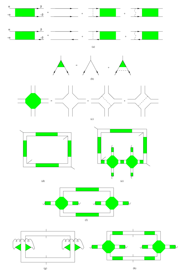
FIG. 1.: Suggested phase diagram in Clogston limit when $\Delta_{0}\tau_{s0}\ll 1$; Insert is the phase diagram of Chandrasekhar-Clogston theory. A superconducting glass phase appears at $H_{SG}=H^{0}_{c}-\delta H_{c}$ with $\delta H_{c}\sim H^{0}_{c}/G^{2}\ln G$. The thick line along $T=0$ axis represents the superconducting glass phase discussed in the paper; the dashed line stands for a possible finite temperature phase transition between the superconducting glass phase and a normal phase.

FIG. 2.: a). Dyson equation for diffusons and Cooperons. Solid lines correspond to electron Green functions in a metal; Dashed lines are for impurity scatterings preserving the spin while the wavy ones for spin orbit scatterings. b).Vertex correction of pair potentials. c). Hikami Box. d),e). Diagrams for the fluctuations of spin polarization energy. f) Diagrams representing the correlation function $\langle\delta K^{0}({\bf r}_{1},{\bf r}_{2})\delta K^{0}({\bf r}_{3},{\bf r}_{4})\rangle$. g),h). Diagrams representing the correlation function of supercurrent densities $\langle{\bf J}_{s}({\bf r}){\bf J}_{s}({\bf r^{\prime}})\rangle$. Solid wavy lines in g). represent the correlation function $\langle\delta\Delta({\bf r}_{1})\delta\Delta({\bf r}_{2})\rangle$ given in Eq. 17.

REFERENCES

- [1] W. Wu, P. W. Adams, Phys. Rev. Lett.74, 610(1995).
- [2] A. A. Abrikosov, Fundamentals of The Theory of Metals, North-Holland, 1988.
- [3] A. M. Clogston, Phys. Rev. Lett.9, 266(1962).
- [4] B. S. Chandrasekhar, Appl. Phys. Lett. 1, 7(1962).
- [5] P. A. Lee, D. Stone, Phys. Rev. Lett.55, 1622(1985).
- [6] B. Altshuler, Pisma Zh. Eksp. Teor. Fiz. 41, 530(1985)[JETP Lett. 41, 648(1985)]
- [7] B. Altshuler, B. I. Shklovskii, Zh. Eksp. Teor. Fiz. 91, 220(1986) [Sov. Phys. JETP. 64, 127(1986)]
- [8] A. M. Finkelshtein, Pisma Zh. Eksp. Teor. Fiz. 45, 37(1987)[JETP Lett. 45, 46(1987)] and references therein.
- [9] S. F. Edwards, P. W. Anderson, J. Phys. F 5, 965(1975).
- [10] B. Altshuler B. Spivak, Zh. Eksp. Teor. Fiz. 92, 609(1987) [Sov. Phys. JETP 65,343(1987)].
- [11] B. Spivak, A. Zyuzin, Pisma Zh. Eksp. Teor. Fiz. 47, 221(1988) [Sov. Phys. JETP Lett. 47, 267(1988)].
- [12] B. Spivak, A. Zyuzin, Mesoscopic fluctuations of Current Density in Disordered Conductors, Mesoscopic Phenomena in Solids edited by B. Altshuler, P. Lee and R. Webb, Elsevier Science Publishers B. V., 1991.
- [13] C. W. J. Beenakker, Phys. Rev. Lett. 67, 3836(1991).
- [14] B. Spivak, F. Zhou, Phys. Rev. Lett. 74, 2800(1995).
- [15] A. Aronov, B. Spivak, Fiz. Tverd. Tela 17, 2806 (1975) [ Sov. Phys. Solid State 17,1874 (1975)]. .
- [16] L. Bulaevski, V. Kuzzi, A. Sobianin, Pisma Zh. Eksp. Teor. Fiz. 25, 314(1977) [JETP Lett. 25, 7(1977)].
- [17] B. Spivak, S. Kivelson, Phys. Rev. B 43, 3740(1991).
- [18] S. Kivelson, B. Spivak, Phys. Rev. B 45,10492(1990).
- [19] F. Zhou, B. Spivak, Phys. Rev. Lett. 80, 5647(1998).
- [20] N. R. Werthamer, E. Helfand, P. C. Hohenberg, Phys. Rev. B 147, 295(1966).
- [21] K. Maki, Phys. Rev. B 148, 362(1966).
- [22] R. A. Ferrell, Phys. Rev. Lett. 3, 262(1959).
- [23] P. W. Anderson, Phys. Rev. Lett. 3, 325(1959).
- [24] A. A. Abrikosov, L. P. Gorkov, Sov. Phys. JETP 15, 752(1962).
- [25] A. A. Abrikosov, L. P. Gorkov, I. E. Dzyaloshinski, Methods of Quantum Field Theory in Statistical Physics, Dover, 1975.
- [26] We want to thank Professor Y. Kagan for raising this issue.
- [27] H. Yoshika, Jour. Phys. Soc. Japan 63, 405(1994).
- [28] J. Villain, Jour. Phys. C 10, 4793(1977).
- [29] Sajeev John, T. C. Lubensky, Phys. Rev. B 34, 4815(1986).
- [30] V. Vinokur, L. Ioffe, A. Larkin, M. Feigelman, Sov. Phys. JETP 66,198(1987).
- [31] M. Fisher, Phys. Rev. Lett. 62, 1415(1989).
- [32] P. Fulde, P. A. Ferrell, Phys. Rev. B 135, A550(1964).
- [33] A. I. Larkin, Yu. N. Ovchinnikov, Zh. Eksp. Teor. Fiz. 47, 1136(1964) [Sov. Phys. JETP 20, 762(1965)]
- [34] L.G. Aslamazov, Zh. Eksp. Teor. Fiz. 55, 1477-1482 (1968) [Sov. Phys. JETP 28, 773(1969)].
- [35] F. Zhou, C. Biagini, Phys. Rev. Lett. 81, 4188(1998).
- [36] I. M. Lifshitz, Adv. Phys. 13, 483(1964).
- [37] B. I. Halperin, M. Lax, Phys. Rev.148, 722(1966).
- [38] J. Zittartz, J. S. Langer, Phys. Rev.148, 741(1966).
- [39] I. E. Smolyarenko, B. L. Altshuler, Phys. Rev. B 55, 10451(1977).
- [40] B. Altshuler, B. Kravtsov, I. Lerner, Sov. Phys. JETP 64,1352(1986).
- [41] B. A. Muzykantskii, D. E. Khmelnitskii, Phys. Rev. B 51, 5480(1995).
- [42] K. Efetov, V. Falko, Phys. Rev. B 52, 17413(1995).
- [43] Strictly speaking, this statement is correct only when the bulk of the distribution function is concerned. In principal, the time reversal symmetry doesn’t exclude the possibility to have negative Josephson couplings. Furthermore, in the presence of prelocalized states, the correlational effect discussed in Ref.15,16 can also lead to a negative superfluid density. However, the probability to find such events is exponential small.
- [44] F. Zhou, C. Biagini, Phys. Rev. Lett. 81, 4724(1998).
- [45] S. Okuma, F. Komori, Y. Ootuka, S. Kobayashi, J. Phys. Soc. Jpn. 52, 2639(1983).
- [46] J. M. Graybeal, M. R. Beasley, Phys. Rev. B 29, 4167(1984).
- [47] R. C. Dynes, A. E. White, J. M. Graybeal, J. P. Garno, Phys. Rev. Lett. 57, 2195(1986).
- [48] A. F. Hebard, M. A. Paalanen, Phys. Rev. Lett. 65, 927(1990).
- [49] Y. Liu, K. A. McGreer, B. Nease, D. B. Haviland, G. Martinez, J. W. Halley and and A. M. Goldman, Phys. Rev. Lett.67, 2068(1991).
- [50] D. Thouless, Phys. Rev. B27, 6083(1983).
- [51] P. Brouwer, Phys. Rev. B58, 10135(1998).
- [52] F. Zhou, B. Spivak, B. Altshuler, Phys. Rev. Lett. 82, 608(1999).
- [53] M. Fisher, Phys. Rev. Lett. 57, 885(1986).
- [54] S. Chakravarty, S. Kivelson, G. Zimanyi, B. Halperin, Phys. Rev. B 35, 7256(1987).
- [55] V.J. Emery, S.A. Kivelson, Phys. Rev. Lett. 74, 3253 (1995).
- [56] S.Sachdev, cond-mat/9705074.
- [57] J. M. Kosterlitz, D. J. Thouless, J. Phys. C 6, 1181(1973).
- [58] B. W. Morris, S. G. Colborne, M. A. Moore, A. J. Bray, J. Canisius, J. Phys. C 19, 1157(1986).