Theory of transient spectroscopy
of multiple quantum well structures

Abstract

A theory of the transient spectroscopy of quantum well (QW) structures under a large applied bias is presented. An analytical model of the initial part of the transient current is proposed. The time constant of the transient current depends not only on the emission rate from the QWs, as is usually assumed, but also on the subsequent carrier transport across QWs. Numerical simulation was used to confirm the validity of the proposed model, and to study the transient current on a larger time scale. It is shown that the transient current is influenced by the nonuniform distribution of the electric field and related effects, which results in a step-like behavior of the current. A procedure of extraction of the QW emission time from the transient spectroscopy experiments is suggested.

I Introduction

Transient spectroscopy of quantum-well (QW) structures allows to study the emission processes from the QWs and thus to obtain information on QW parameters, such as the energy spectrum, photoionization cross-section, tunneling escape time, etc. [1, 2, 3] This technique is based on an analysis of the transient current or capacitance relaxation upon the application of a large-signal bias across the QW structure. It complements admittance spectroscopy, which studies the ac current in the QW structure upon application of a small-signal voltage. [4] The transient spectroscopy of QWs has many similarities with the deep level transient spectroscopy (DLTS) [5] and enables a simple theory to be derived for use in the processing of experimental data. [3] However, there is an important difference in the carrier capture by deep levels and that involving QWs. In the latter case, the presence of a continuous energy spectrum for the in-plane motion in the QW allows the capture by emission of a single optical phonon rather than by a multi-phonon processes typical for deep levels. [6] As a result, the corresponding capture times are several orders of magnitude less than for deep levels and often do not exceed a few picoseconds. [7] This quantitative difference results in serious qualitative consequences. The processes of carrier transport between neighboring QWs can no longer be considered as infinitely fast. These processes may play a decisive role in the relaxation kinetics changing noticeably the formulae of a simple theory, similar to the case of structures with very high concentration of deep levels. [8] In this work we present a theoretical description of the transient spectroscopy of QWs and discuss its possible applications. We obtain more general analytical expressions for the parameters of the transient current than those of Ref. [3]. The analytical model is confirmed by numerical simulation, and the procedure of the extraction of the QW parameters from experimental data is discussed.

II Analytical model

We consider a QW structure containing $M$ QWs (n-doped at sheet density $N_{D}$) of width $L_{w}$ separated by undoped barriers of width $L_{b}$ large enough to prevent inter-well tunneling (see Fig. 1). This structure is typical for quantum well infrared photodetectors (QWIPs). [9] The QW structure is provided with a heavily doped (Ohmic) collector and a blocking emitter contact (for example, containing a Schottky barrier or p-n junction) which is often used to avoid DC current and thus to simplify the interpretation of experimental data. [3]

During the first period of the transient spectroscopy experiment, [3] the forward bias is applied to the emitter, and all QWs are filled by electrons with the equilibrium sheet density $N_{0}\approx N_{D}$. In the second period, a large reverse bias $V$ is applied to extract electrons from the QWs, and transient current is recorded. The problem has some similarities with the treatment presented for the kinetics of electron packet in a system of undoped QWs. [10]. Immediately after the application of $V$, the electric field in the QW structure is uniform and given by $E_{0}=(V+V_{bi})/L$, where $V_{bi}$ is the built-in voltage between the emitter and collector, and $L=ML_{w}+(M+1)L_{b}\approx(M+1)L_{b}$ is the structure thickness. This field causes fast removal of delocalized electrons from the structure at almost fixed $N_{0}$. This is a very fast (on a ps time scale) component of the transient current [11] limited by carrier capture and transit times, which is manifested as an instantaneous current step in the case of limited time resolution of a measurement setup. We shall be interested here in a subsequent slow current relaxation caused by the QW recharging. The initial part of this relaxation (after completion of the fast transient) can be easily calculated.

In the presence of external illumination, the emission rate from the $i$-th QW with electron density $N_{i}$ is $GN_{i}={\sigma\Phi N_{i}+\gamma\exp[(\varepsilon_{f}-\varepsilon_{i})/kT]}$, where $\sigma$ is the photoionization cross-section, $\Phi$ is the incident photon flux, $\varepsilon_{i}$ is the QW ionization energy, $\varepsilon_{f}(N_{i})$ is the Fermi energy of the electrons in the QW, and $\gamma$ is the thermoionization coefficient. In our estimates and further numerical simulations, we shall restrict our analytical calculations to the case of relatively low temperatures or high light intensities giving $G\cong\sigma\Phi$. This restriction is not compulsory since all analytical formulae are applicable for an arbitrary relation between the optical and thermal generation.

We assume that the carriers emitted from the QWs drift with a constant velocity $v_{d}$ towards the collector. While traversing a QW, carriers are captured by the QW with a probability $p$ ($0<p\leq 1$). Carriers emitted from the $k$-th QW give the following contribution to the carrier concentration in the $i$-th barrier (between $i$-th and $(i+1)$-th QWs):

$$n_{ki}=\frac{GN_{k}}{v_{d}}\,(1-p)^{i-k},\qquad(i\geq k).$$ (1)

The total concentration in the $i$-th barrier $n_{i}$

$$n_{i}=\sum_{k=1}^{i}n_{ki}=\frac{G}{v_{d}}\sum_{k=1}^{i}N_{k}(1-p)^{i-k}.$$ (2)

Since the change of a QW charge is determined by the balance between carrier capture and emission, we can, with the help of Eq. (2), obtain the system determining the kinetics of all $N_{i}$:

$$\frac{dN_{i}}{dt}=-GN_{i}+n_{i-1}v_{d}\,p=G\left[-N_{i}+\sum_{k=1}^{i-1}N_{k}p(1-p)^{i-1-k}\right]$$ (3)

and, hence, of the current in the external circuit $I(t)$ which could be expressed in terms of $N_{i}(t):$

$$I(t)=\frac{ev_{d}}{M+1}\sum_{i=1}^{M}n_{i}=\frac{eG}{M+1}\sum_{i=1}^{M}\sum_{k=1}^{i}N_{k}(t)(1-p)^{i-k}.$$ (4)

In principle, we can obtain analytical (though rather cumbersome) solution of the linear system of Eq. (3) for an arbitrary $t$. However, it would not be correct. The change in $N_{i}$ causes re-distribution of the electric field and, hence, of the drift velocity in the system. This means that $v_{d}$ is no longer constant but changes from point to point in an unknown way so that the behaviour of $I(t)$ remains unknown. That is why we restrict ourselves to the initial stage of the slow relaxation when we can still assume that in the right-hand side of Eq. (3) $N_{i}=N_{0}$ and $v_{d}={\rm const}.$ This gives

$$\frac{dN_{i}}{dt} = -GN_{0}(1-p)^{i-1};$$ (5)

$$I(0) = \frac{I_{e}}{p(M+1)}\left\{1-\frac{1-p}{pM}\left[1-(1-p)^{M}\right]\right\};$$ (6)

$$\frac{dI}{dt}(0) = -\frac{GI_{e}}{p^{2}M(M+1)}\left[1-(1+Mp)(1-p)^{M}\right]$$ (7)

where $I_{e}=eGN_{0}M$ is the total emission rate from all QWs. Eqs. (6),(7) give us the relaxation time constant (inverse normalized slope of the current):

$$\tau=-\left(\frac{dI/dt}{I}\right)^{-1}=\frac{pM-(1-p)[1-(1-p)^{M}]}{G\left[1-(1+pM)(1-p)^{M}\right]}.$$ (8)

In the most interesting case, when $p\ll 1$ and $M\gg 1$ (which corresponds to practical QWIPs), parameters $I_{0}$ and $\tau$ are expressed as:

$$I_{0} = I_{e}\times g[1-g(1-\exp(-1/g))],$$ (9)

$$\tau = \frac{1}{G}\times\frac{1-g[1-\exp(-1/g)]}{g[1-(1+1/g)\exp(-1/g)]},$$ (10)

where $g=1/(pM)$ is a transport parameter. If we characterize QW capture processes by the capture time $\tau_{c}$ or the capture velocity $v_{c}=L_{p}/\tau_{c}$, which is related to capture probability as $p=1/(1+v_{d}/v_{c})$, [12, 13] then $g=\tau_{c}/\tau_{tr}+1/M\approx\tau_{c}/\tau_{tr}$, where $\tau_{tr}=L/v_{d}$ is the transit time. Therefore, the parameter $g$ corresponds to the photocurrent gain of a QWIP.[9]

It should be noted that the amplitude of the transient current $I_{0}$ is equal to the amplitude of the fast transient (primary photocurrent) in a photoexcited QWIP. [11] In general, the time constant for the transient current $\tau$ is determined not only by the emission time $1/G$, but also by a transport parameter $g,$ similarly to the case of DLTS for a very high concentration of deep centers.[8] Particularly, in the case $g\ll 1$ we have $\tau\approx 1/(gG)\gg 1/G$. Hence, one cannot obtain the photoionization cross-section from the transient spectroscopy experiment ignoring the correction factor (see Eqs. (8)–(10)) dependent on $g$. Only in the limiting case $g\gg 1$ (or $pM\ll 1$), the relaxation time tends to $1/G$ which corresponds to the simple model of Ref. [3]. To fulfill this condition, one has to use QW structure with small capture probability and small number of QWs. In this case $I_{0}=0.5\times I_{e}$, which corresponds to a high-frequency gain value of 0.5 for extrinsic photoconductors and QWIPs with large value of the low-frequency gain $g$. [11, 14, 15] Note that the capture probability $p$ is a function of the electric field, decreasing with field, so that the simplified approach predicting $\tau=1/G$ can be accurate at high fields, but inaccurate at low fields.

We point out that the value of the photocurrent gain $g$ can be determined from the transient photocurrent in QWIP illuminated by a step-like infrared radiation, where the ratio of the amplitude of the fast transient to the steady-state photocurrent is equal to $\{1-g[1-\exp(-1/g)]\}$. [11]

III Numerical simulation

The model presented above is justified only for the initial part of the transient, since we neglected the modulation of the electric field due to the QW recharging. To check this model and to obtain a description of the transient current for a wider time interval, we also studied the transient processes using numerical simulation. A time dependent QWIP simulator [11, 16] was used with a zero-current boundary condition for the reverse-biased emitter contact. We simulated the transient spectroscopy experiment of Ref. [3] on GaAs/Al_0.25Ga_0.75As QW structure with the area $S=2\times 10^{-4}$ cm^-2 containing 10 donor-doped QWs with $L_{w}=$60 Å QWs and $N_{D}=5\times 10^{11}$ cm^-2, undoped barriers with $L_{b}=$350 Å, Schottky emitter contact ($V_{bi}=0.75$ V) and collector GaAs contact doped with donors at 10¹⁸ cm${}^{-3}.$ The photoexcitation conditions were similar to those used in the experiment. [3]

Figure 2(a) shows the transient current calculated for a reverse bias of 1 V, which for the given $V_{bi}$ corresponds to the applied field $E_{0}\approx$40 kV/cm. The capture probability was chosen to be $p=0.04$ so that $g=2.5$. The initial part of the transient ($t\lesssim\tau^{\prime}$ where $\tau^{\prime}\approx 43$ $\mu$s is the position of the first step in Fig. 2(a)) is very well described by an exponential function with the amplitude and time constant calculated by our analytical model without any fitting parameters. The time constant obtained is $\tau\approx 345$ $\mu$s, while the emission time is somewhat smaller, $1/G=300$ $\mu$s.

Starting from the time moment $t=\tau^{\prime}$, the transient current decays more rapidly, and displays a series of steps and shoulders. These features are due to the redistribution of the electric field caused by the depleting of QWs (see Fig. 2(b,c)). The $i$-th step occurs when the electric field in the $(M+1-i)$-th barrier becomes zero. When this happens, the electron density in the $(M+1-i)$-th QW returns to its equilibrium value $N_{0}$, and this well does not contribute to the emission current. The electron transport in the region between this QW and collector is purely diffusive. Using Eq. (5) and the condition of zero electric field in the $M$-th barrier $E_{0}=\sum_{i=1}^{M}\frac{e\Delta N_{i}}{\varepsilon\varepsilon_{0}}\frac{i}{M+1}$ ($\varepsilon\varepsilon_{0}$ is the dielectric constant), we obtain the following estimate for the time constant $\tau^{\prime}$:

$$\tau^{\prime}\approx\frac{\varepsilon\varepsilon_{0}E_{0}}{e\,GN_{0}M}\,\frac{1}{g^{2}\,[1-(1+1/g)\exp(-1/g)]}.$$ (11)

For the case of Fig. 2 this estimate gives $\tau^{\prime}\approx 39$ $\mu$s, which is in a good agreement with the results of numerical calculations ($\tau^{\prime}\approx 43$ $\mu$s).

Since $\tau^{\prime}\ll\tau$ (unless $g$ is very small), only a small initial part of the transient process is described by the exponential function with time constant $\tau$ and amplitude $I_{0}$. Thus, the fitting of experimental data by an exponential function to extract the time constant $\tau$ should be done over the interval $0\lesssim t<\tau^{\prime}$. The fitting over longer time intervals can result in a significant error in estimating $\tau$ (the dashed line on Fig. 2(a) is an “intuitive” exponential fitting with the time constant $\tau=130$ $\mu$s). It should be stressed that the measurement circuit should have $RC$-time constant ($R$ is the load resistance and $C$ is the QW structure high-frequency capacitance) much smaller than time constant $\tau^{\prime}$ for correct evaluation of $\tau$.

To check the influence of the QW capture velocity $v_{c}$ on the time constant $\tau$, we simulated the transient response for different values of $v_{c}$. The values of the amplitude and time constant of the initial part of the transient current extracted from numerical simulation are shown in Fig. 3. A good agreement between these results and formulas Eq. (6),(8) proves the validity of the analytical model.

So far we have assumed that the photoionization cross-section (or emission rate) is independent of the local electric field. While this is a good approximation for bound-to-continuum transitions, the photoionization cross section for bound-to-bound and bound-to-quasi-bound transitions depends strongly on electric field. [9] To investigate this effect, we compared the results of simulation for the cases of field-dependent and field-independent cross-section (see Fig. 4). We used the model of the field-dependent cross-section proposed in Ref. [3]:

$$\sigma(E)=\sigma_{0}\times 0.5\text{\thinspace erfc}[(\varepsilon_{2}-eEL_{w}/2)/(\sqrt{2}\Delta\varepsilon)],$$ (12)

where $\sigma_{0\text{ }}$is the optical cross-section, erfc($x$) is the complementary error function, $\varepsilon_{2}$ is the ionization energy of the second level, and $\Delta\varepsilon$ is the variance of $\varepsilon_{2}$ due to fluctuations. [3] The values $\varepsilon_{2}=4$ meV and $\Delta\varepsilon=3.5$ meV also taken from Ref. [3], were used. It is seen from Fig. 4 that the field dependence of cross-section washes out steps on the $I(t)$ curve. Moreover, the initial part of the curve, $0<t<\tau^{\prime},$ deviates significantly from an exponential function of the analytical model. Physically, this is caused by the decrease of the photoemission current from near-collector QWs due to the electric field redistribution. This effect makes the extraction procedure of the time constant $\tau$ from the slope of the transient current more complicated. However, the transient current amplitude $I_{0}$ is not affected by the field redistribution. Since the amplitude is directly related to the photoemission current ($I_{0}=0.5I_{e}$) in the case $g\gg 1$, we propose to use the amplitude of the transient current rather than its slope to extract the photoionization cross-section from experimental data.

IV Conclusions

A theory of the transient spectroscopy of QW structures is presented. Analytical expressions for the initial stage of relaxation current are derived. It is shown that the time constant of the transient current is a function of both the photoionization cross-section and the transport parameter $g$ becoming $g$-independent at $g\gg 1$. Numerical simulation is used to check the validity of the analytical model and study the transient current in more detail. The procedure of extraction the QW emission rate from the experimental data is discussed.

This work is supported in part by the NSF under Grant No. ECS-9809746. H. R. and A. S. also gratefully acknowledge the support of NSERC.

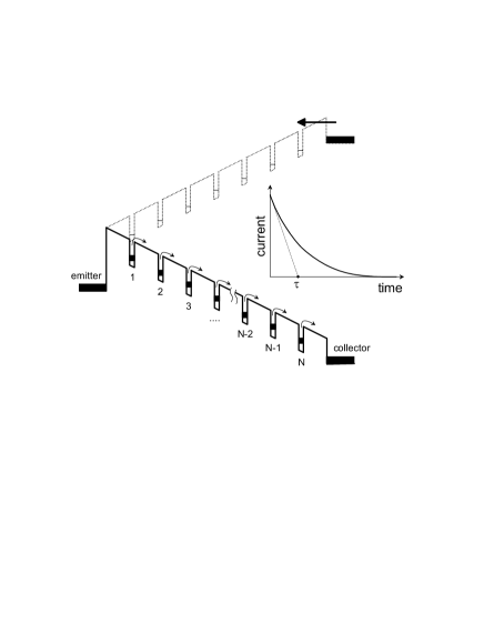
FIG. 1.: Schematic illustration of the conduction band diagram and the transient current in the transient spectroscopy experiment.

FIG. 2.: (a) Transient current, (b) electron density in QWs, and (c) electric field in the barriers for structure with 10 QWs. In (a), solid line – numerical simulation, dashed line - analytical model, and dotted line – exponential fitting of the transient current on a large time scale. In (b) and (c), labels indicate the index of the QW and barrier, respectively.

FIG. 3.: Dependence of the inverse normalized time constant $G/\tau$ and amplitude of the transient current $I_{0}/I_{e}$ on the value of gain $g$. Solid lines – analytical model, markers – numerical simulation.

FIG. 4.: Comparison of the transient currents for the cases of the field-dependent (solid line) and field-independent (dashed line) photoionization cross-sections. The inset shows the field dependence of the photoionization cross-section.

REFERENCES

- [1] P. A. Martin, K. Meehan, P. Gavrilovic, K. Hess, N. Holonyak, and J. J. Coleman, J. Appl. Phys. 54, 4689 (1983).
- [2] E. Martinet, E. Rosencher, F. Chevoir, J. Nagle, and P. Bois, Phys. Rev. B 44, 3157 (1991).
- [3] F. Luc, E. Rosencher, and P. Bois, Appl. Phys. Lett. 62, 2542 (1993).
- [4] D. V. Lang, M. B. Panish, F. Capasso, J. Allam, R. A. Hamm, A. M. Sergent, and W. T. Tsang, Appl. Phys. Lett. 50, 736 (1987).
- [5] D. V. Lang, J. Appl. Phys. 45, 3023 (1974).
- [6] V. N. Abakumov, V. I. Perel, and I. N. Yasievich, Sov. Phys. Semicond. 12, 1 (1978).
- [7] P. W. M. Blom, C. Smit, J. E. M. Haverkort, and J. H. Wolter, Phys. Rev. B 47, 2072 (1993).
- [8] A. Y. Shik, Sov. Phys. Semicond. 18, 1100 (1984).
- [9] B. F. Levine, J. Appl. Phys. 74, R1 (1993).
- [10] A. M. Georgievskii, V. A. Solov’ev, B. S. Ryvkin, N. A. Strugov, E. Yu. Kotel’nikov, V. E. Tokranov, and A. Ya. Shik, Semiconductors 31, 378 (1997).
- [11] M. Ershov, Appl. Phys. Lett. 69, 3480 (1996).
- [12] E. Rosencher, B. Vinter, F. Luc, L. Thibaudeau, P. Bois, and J. Nagle, IEEE J. Quantum Electron. 30, 2875 (1994).
- [13] V. D. Shadrin, V. V. Mitin, V. A. Kochelap, and K. K. Choi, J. Appl. Phys. 77, 1771 (1995).
- [14] S. A. Kaufman, N. S. Khaikin, and G. T. Yakovleva, Sov. Phys. Semicond. 3, 485 (1969).
- [15] M. M. Blouke, E. E. Harp, C. R. Jeffus, and R. L. Williams, J. Appl. Phys. 43, 188 (1972).
- [16] M. Ershov, V. Ryzhii, and C. Hamaguchi, Appl. Phys. Lett. 67, 3147 (1995).