A Non-Crossing Approximation for the Study of Intersite Correlations

Abstract

We develop a Non-Crossing Approximation (NCA) for the effective cluster problem of the recently developed Dynamical Cluster Approximation (DCA). The DCA technique includes short-ranged correlations by mapping the lattice problem onto a self-consistently embedded periodic cluster of size $N_{c}$. It is a fully causal and systematic approximation to the full lattice problem, with corrections ${\cal{O}}(1/N_{c})$ in two dimensions. The NCA we develop is a systematic approximation with corrections ${\cal{O}}(1/N_{c}^{3})$. The method will be discussed in detail and results for the one-particle properties of the Hubbard model are shown. Near half filling, the spectra display pronounced features including a pseudogap and non-Fermi-liquid behavior due to short-ranged antiferromagnetic correlations.

1 Introduction

One of the most challenging tasks in theoretical condensed matter physics is the description of strongly correlated electron systems. The Coulomb interaction between electrons plays a dominant role in these systems and usually strongly influences the electronic properties and the physics of the ground-state phase. The discovery of heavy Fermion systems in the late seventies HFreviews and high-$T_{c}$ super-conductors ten years later high_Tc has stimulated strong experimental and theoretical interest in this field. However, despite a multitude of attempts to describe such strongly correlated electron systems theoretically, a complete understanding of the observed rich physics has not yet been accomplished. Even the simplest model for strongly correlated electron systems, the Hubbard model (HM), must be considered unsolved in more than one dimension lieb_wu after almost forty years of intensive study. Exact diagonalization or quantum Monte-Carlo studies for two or three dimensions are restricted to small lattice sizes and predictions for the thermodynamic limit are maybe problematic dagotto_review .

However, in the limit of infinite dimensions $D=\infty$, correlated lattice models undergo a significant simplification. Their dynamics become purely local and therefore the lattice problem can be mapped onto a generalized single impurity Anderson model coupled to a host, which has to be determined self-consistently Bra_Mie ; Janis ; Jarr92 ; Geo_Kot . The Dynamical Mean Field Approximation used in the context of real materials thus assumes that only local dynamics are present. Despite the neglect of nonlocal correlations, this method has been shown to capture several important features of e.g. the Hubbard model Jarr92 ; jarrell92 ; TP95 . Nevertheless it has some significant shortcomings due to the mapping onto a purely local model. For instance, it does not include the effect of nonlocal correlations like antiferromagnetic spin fluctuations on the one-particle properties, and is not capable of describing nonlocal order parameters. However, both effects are believed to be especially important for a description of the High-$T_{c}$ materials. Here the one-particle spectra have shadow bands due to short-ranged antiferromagnetic fluctuations, preformed pseudogaps due to superconducting or spin fluctuationsshadow ; preformed0 ; preformed1 ; preformed2 ; preformed3 , and the superconducting order parameter is of nonlocal ($d$) character.

In order to include these types of nonlocal dynamics into the theory there have been several efforts to add so-called $\frac{1}{D}$ corrections to the DMFA Dongen ; Schi_Ing ; obermeier . However, these methods either experience causality problems Dongen ; Schi_Ing (because of the necessary inclusion of nonlocal Green functions in self-energy diagrams which do not have a negative semidefinite imaginary part), or are restricted to the calculation of a few moments of the spectral function moments .

These shortcomings do not apply to the Dynamical Cluster Approximation (DCA). This method systematically includes nonlocal short-ranged correlations while preserving causality hettler1 ; hettler2 . The DCA is a scheme which maps the lattice problem onto a self-consistently embedded effective finite-size cluster model. Due to the finite size of the cluster, nonlocal corrections to the local dynamics can be systematically included as the cluster size increases. The basic idea of the DCA is to take into account nonlocal physics by calculating the self energy at selected points $\bf K$ in the Brillouin zone and consider the self energy at these points to represent the self-energy in the surrounding of these points ${\bf K}+{\bf k}^{\prime}$: $\Sigma({\bf K})\approx\Sigma({\bf K}+{\bf k}^{\prime})$. The theory then maps the lattice problem onto an effective finite-size system with periodic boundary conditions coupled to an external bath and the resulting system is solved self-consistently. The DCA has two well defined limits: It recovers the DMFA as the cluster size goes to 1 and becomes the exact solution for the model under consideration as the cluster size goes to infinity.

The use of the DCA as an approximation can be justified as long as the momentum dependence of the self-energy of the real system is weak. This is obviously realized in high spatial dimensions where a coarse grid of $\bf K$-points should capture all the basically short-ranged dynamics. In two- or three-dimensional systems the approximation is more crude, but can be motivated by the observation that the dominant structures in the one-particle dynamics are generated by local renormalizations, while nonlocal effects only lead to minor renormalizations of these structures. Note that this assumption automatically inhibits studies very close to phase transitions since there strong, long-ranged fluctuations must be expected. However, sufficiently away from phase boundaries correlated systems indeed show only mild momentum dependence of the one-particle self energy as compared to its frequency dependence.

So far only Quantum Monte Carlo simulations and exact enumeration have been used to solve this problem of a cluster in an external bath hettler2 ; hettler1 . In the DMFA the NCA has successfully been applied to the effective single impurity problem pruschke ; pruschke2 ; obermeier1 ; schmalian2 ; Maier . In this paper we introduce an extended version of the NCA to solve the effective periodic cluster model of the DCA.

The paper is organized as follows. First a short review of the DMFA is given, which is reproduced by the DCA for a single site cluster. Then we provide a microscopic definition of the DCA in terms of its Laue function, and rederive the DCA algorithm using Baym’s $\Phi$ functional formalism. We then define the effective cluster model onto which the lattice system is mapped by the DCA. An extended version of the NCA applicable to an impurity cluster of arbitrary size is discussed in detail and finally results for the one-particle properties of the Hubbard model are shown and compared to corresponding results of the DMFA.

2 Dynamical Mean Field Approximation

In this paper we consider the single-band Hubbard model described by the Hamiltonian

$$H=\sum_{ij\sigma}t_{ij}c^{\dagger}_{i\sigma}c_{j\sigma}+U\sum_{i}n_{i\uparrow}n_{i\downarrow}\quad\mbox{,}$$ (1)

where $c_{i\sigma}^{\dagger}$ ($c_{i\sigma}$) creates (destroys) an electron at site $i$ with spin sigma and $n_{i\sigma}$ are the corresponding number operators. Lattice models of this kind simplify significantly in infinite dimensions, while retaining their full local dynamics. Metzner and Vollhardtmetzner showed that the necessary rescaling of the kinetic energy as $1/\sqrt{D}$ leads to a collapse of all nonlocal diagrams in a skeleton expansion for the self-energy. Consequently the corresponding Baym-Kadanoff $\Phi$ functional can be expressed in terms of local quantities only.

Müller-Hartmann MueHa89 was able to deduce the same result by inspecting the momentum dependence of vertices in diagrammatic approaches as $D\rightarrow\infty$. For Hubbard-like models, the momentum dependence of each vertex in a diagrammatic expansion of the functional $\Phi$ is completely characterized by the Laue function

$$\Delta({\bf k}_{1},{\bf k}_{2},{\bf k}_{3},{\bf k}_{4})=\sum_{\bf r}e^{i({\bf k}_{1}-{\bf k}_{2}+{\bf k}_{3}-{\bf k}_{4})}\quad\mbox{,}$$ (2)

where ${\bf k}_{1}$ and ${\bf k}_{3}$ (${\bf k}_{2}$ and ${\bf k}_{4}$) are the momenta entering (leaving) the vertex. In a conventional diagrammatic approach $\Delta({\bf k}_{1},{\bf k}_{2},{\bf k}_{3},{\bf k}_{4})=N\delta_{{\bf k}_{1}+{\bf k}_{3},{\bf k}_{2}+{\bf k}_{4}}$, which expresses momentum conservation on the vertex. However as $D\to\infty$ Müller-Hartmann showed that the Laue function reduces to

$$\Delta_{D\rightarrow\infty}({\bf k}_{1},{\bf k}_{2},{\bf k}_{3},{\bf k}_{4})=1+{\cal O}(1/D)\quad\mbox{.}$$ (3)

The DMFA assumes the same Laue function (3) even in the context of finite dimensions. Therefore both the infinite-dimensional theory and the DMFA neglect momentum conservation at the internal vertices of irreducible diagrams and the momenta in the corresponding $\Phi_{DMFA}$ functional may be freely summed over the whole Brillouin zone. This leads to a collapse of the momentum dependent contributions to the functional $\Phi_{DMFA}$ and only local terms remain. This is illustrated in Fig. 1 for a second order diagram.

Figure 1: The Laue function (3) leads to a collapse of the momentum dependence of the DMFA Baym-Kadanoff $\Phi_{DMFA}$ functional, illustrated for a second order contribution.

The self-energy (a functional derivative of the functional $\Phi_{DMFA}$ with respect to a Green function leg) also becomes a functional of local propagators only and therefore becomes a constant in momentum space. Consequently the lattice problem can be mapped onto an effective impurity problem.

The DMFA has proven to capture the key features of strongly correlated electron systems and to provide insight in the complicated dynamics mediated by correlations. Despite its great success in the description of correlated electron systems the DMFA has some significant shortcomings due to the neglect of non-local dynamics.

3 Dynamical Cluster Approximation

The DCA extends the DMFA through the inclusion of short-ranged dynamical correlations. The DCA was introduced and discussed in detail in hettler1 ; hettler2 . In this paper we will rederive the DCA algorithm with an argument which is complimentary to that used by Müller-Hartmann MueHa89 to describe the DMFA.

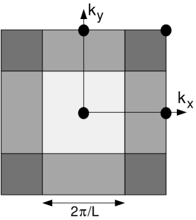
Figure 2: The cluster momenta K (filled circles) and coarse graining cells (different fill patterns) for a $N_{c}=4$ cluster in the Brillouin zone of a two dimensional lattice. The cells adjacent to the Brillouin zone boundary extend periodically to the opposite site.

The basic idea of the DCA is to partially restore the momentum conservation relinquished by the DMFA. To this end the Brillouin-zone is divided into $N_{c}=L^{D}$ cells of size $(2\pi/L)^{D}$ (see Fig. 2). Each cell is represented by a cluster momentum $\bf K$ in the center of the cell. We require that momentum conservation is (partially) observed for momentum transfers between cells, i.e. for momentum transfers larger than $\Delta k=2\pi/L$, but neglected for momentum transfers within a cell, i.e less than $\Delta k$. This requirement can be established by using the Laue function hettler2

$$\Delta_{DCA}=N_{c}\delta_{{\bf M}({\bf k}_{1})+{\bf M}({\bf k}_{3}),{\bf M}({\bf k}_{2})+{\bf M}({\bf k}_{4})}\quad\mbox{,}$$ (4)

where ${\bf M}({\bf k})$ is a function which maps ${\bf k}$ onto the cluster momentum ${\bf K}$ of the cell containing $\bf k$. With this choice of the Laue function the momenta of each internal leg in the corresponding functional $\Phi_{DCA}$ may be freely summed over the cell and each leg is replaced by the coarse grained average

$$\bar{G}({\bf K})=\frac{N_{c}}{N}\sum_{\tilde{\bf k}}G({\bf K}+\tilde{\bf k})\quad\mbox{.}$$ (5)

This is schematically illustrated in Fig. 3.

Figure 3: The DCA choice of the Laue function (4) leads to the replacement of the lattice propagators $G({\bf k}_{1})$, $G({\bf k}_{2})$, … by coarse grained propagators $\bar{G}({\bf K})$, $\bar{G}({\bf K}^{\prime})$, … (Eq. 5) in the internal legs of $\Phi_{DCA}$, illustrated for a second order diagram.

The coarse grained Green function $\bar{G}({\bf K})$ and corresponding self-energy $\bar{\Sigma}({\bf K})$

$$\bar{\Sigma}({\bf K})=\frac{N_{c}}{N}\sum_{\tilde{\bf k}}\Sigma({\bf K}+\tilde{\bf k})$$ (6)

are functions of the cluster momenta ${\bf K}$ only. The $\tilde{\bf k}$ summation in (5) and (6) runs over the $N/N_{c}$ momenta of the cell about the cluster momentum $\bf K$ and $G$ ($\Sigma$) is the full lattice propagator (self-energy).

With this definition of $\Delta_{DCA}$, the DCA estimate of the Baym-Kadanoff functional $\Phi_{DCA}$ becomes hettler2

$$\Phi_{DCA}(\bar{G})=\sum_{l}\frac{1}{2l}{\rm tr}\left[\bar{\Sigma}^{(l)}\bar{G}\right]$$ (7)

where $\bar{\Sigma}^{(l)}$ is the set of irreducible, coarse grained self-energy diagrams of $l^{\rm th}$ order in the interaction $U$ and the trace indicates summation over frequency, cluster momenta and spin. The DCA result for the free energy of the lattice is

$$\Omega_{DCA}=-k_{B}T(\Phi_{DCA}-{\rm tr}\Sigma G-{\rm tr}\,{\rm ln}[-G])\quad\mbox{.}$$ (8)

$\Omega_{DCA}$ is stationary with respect to the lattice Green function $G$

$$\frac{\delta{\Omega}_{DCA}}{\delta G}=k_{B}T[-\bar{\Sigma}+\Sigma]=0\quad\mbox{,}\,$$ (9)

if $\bar{\Sigma}$ is taken as an approximation for the self-energy $\Sigma$ of the full lattice Green function $G$ (the left hand side of (9) follows from $\delta\bar{G}_{\bf K}/\delta G_{\bf k}=\delta_{{\bf K},{\bf M}({\bf k})}$ and $\delta\Phi_{DCA}/\delta\bar{G}=\bar{\Sigma}$). We have shown previously that $\Sigma=\bar{\Sigma}+{\cal{O}}(1/N_{c})$ in two dimensions and includes dynamical intersite correlations of range $\pi/\Delta k=L/2$ hettler2 .

The coarse grained Green function (5) then takes the form

$$\bar{G}({\bf K},z)=\frac{N_{c}}{N}\sum_{\tilde{\bf k}}\frac{\displaystyle 1}{\displaystyle z-\epsilon_{{\bf K}+\tilde{\bf k}}+\mu-\bar{\Sigma}({\bf K},z)}\quad\mbox{,}$$ (10)

where the self-energy at momentum ${\bf k}={\bf K}+\tilde{\bf k}$, $\Sigma({\bf k})$ is replaced by its coarse grained average $\bar{\Sigma}({\bf K})$ and $z=\omega+i\delta$. Note that the choice of the coarse grained Green function (10) has two well defined limits with respect to the cluster size $N_{c}$. For $N_{c}=1$ the $\tilde{\bf k}$ summation runs over the entire first Brillouin-zone, $\bar{G}$ is the local Green function, thus the DMFA algorithm is recovered. When $N_{c}=\infty$ the $\tilde{\bf k}$ summation vanishes and the DCA becomes equivalent to the exact solution of the Hubbard model.

In order to apply the NCA to solve the effective cluster problem it is convenient to write the coarse grained Green function (10) in a more suitable form. We use the independence of the self-energy $\bar{\Sigma}({\bf K})$ on the integration variable $\tilde{\bf k}$ to write $\bar{G}$ in the form

$$\bar{G}({\bf K},z)=\frac{\displaystyle 1}{\displaystyle z-\bar{\epsilon}_{\bf K}+\mu-\bar{\Sigma}({\bf K},z)-\Gamma({\bf K},z)}\quad\mbox{,}$$ (11)

where ${\rm Im}\Gamma({\bf K})<0$ (see Appendix A). This is just the Green function of an effective cluster model with periodic boundary conditions coupled to a Fermionic bath described by the host function $\Gamma({\bf K})$. Hence we can obtain the coarse grained self energies $\bar{\Sigma}({\bf K})$ by solving a generalized cluster model.

The DCA cluster problem may then be solved by iteration. The iteration loop starts with a guess for the initial cluster self-energy. By computing the coarse grained lattice Green function (10) we get the input quantities for the effective cluster model. The effective dispersion $\bar{\epsilon}_{\bf K}$ is given by the average

$$\bar{\epsilon}_{\bf K}=\frac{N_{c}}{N}\sum_{\tilde{\bf k}}\epsilon_{{\bf K}+\tilde{\bf k}}$$ (12)

and the cluster electrons are coupled to the host function $\Gamma({\bf K})$. This will be described in more detail in section 4 and 5. Given the effective dispersion $\bar{\epsilon}_{\bf K}$ and the host $\Gamma({\bf K})$ the interacting Green function $G_{c}({\bf K})$ of the effective cluster model can be calculated by some suitable method. The cluster self energy is then obtained via $\Sigma_{c}({\bf K},z)=z-\bar{\epsilon}_{\bf K}+\mu-\Gamma({\bf K},z)-G_{c}^{-1}({\bf K},z)$ and the iteration closes by calculating a new $\bar{G}({\bf K})$ with Eq. 10. This procedure is repeated until $G_{c}({\bf K})=\bar{G}({\bf K})$ within the desired accuracy.

4 Effective Cluster Model

To solve the cluster problem with the NCA, we must first define a Hamiltonian for the cluster. The parameters of the Hamiltonian are given by the Green function (11). The corresponding cluster Hamiltonian

$$H_{cluster}=H_{loc}+H_{med}$$ (13)

is most conveniently constructed in momentum space. Its local part is given by

$$H_{loc} = \sum_{{\bf K}\sigma}\bar{\epsilon}_{\bf K}f^{\dagger}_{{\bf K}\sigma}f_{{\bf K}\sigma}$$ (14)

$$+ \frac{U}{N_{c}}\sum_{\stackrel{{\scriptstyle{\bf K},{\bf K}^{\prime}}}{{\bf Q}}}f^{\dagger}_{{\bf K}+{\bf Q}\uparrow}f_{{\bf K}\uparrow}f^{\dagger}_{{\bf K}^{\prime}-{\bf Q}\downarrow}f_{{\bf K}^{\prime}\downarrow}\quad\mbox{,}$$

where $f^{\dagger}_{{\bf K}\sigma}$ ($f_{{\bf K}\sigma}$) creates (destroys) an electron with momentum $\bf K$ and spin $\sigma$. $U$ is the local Coulomb repulsion for two electrons residing on the same cluster site. Since this interaction is local, it is unchanged by the coarse-graining procedurehettler2 . Note that the effective dispersion $\bar{\epsilon}_{\bf K}$ of the cluster states is given by the average bare dispersion in the cell (12). The coupling of the local cluster states with the host has the form

$$H_{med} = \frac{1}{\sqrt{N}}\sum_{{\bf K},{\bf k}^{\prime}\sigma}V_{{\bf K},{\bf k}^{\prime}}(f^{\dagger}_{{\bf K}\sigma}c_{{\bf K}+{\bf k}^{\prime}\sigma}+h.c.)$$ (15)

$$+ \sum_{{\bf k}\sigma}\varepsilon_{\bf k}c^{\dagger}_{{\bf k}\sigma}c_{{\bf k}\sigma}\quad\mbox{,}$$

where $c^{\dagger}_{{\bf K}+{\bf k}^{\prime}}$ ($c_{{\bf K}+{\bf k}^{\prime}}$) describe the effective medium in terms of free fermions with a dispersion $\varepsilon_{\bf k}$. Note that in contrast to the single impurity model, the local states given by $f^{\dagger}_{{\bf K}\sigma}$ couple only to fermions with momenta ${\bf k}={\bf K}+{\bf k}^{\prime}$ within the cell about the cluster momentum ${\bf K}$. Therefore the corresponding hybridization function

$$\Gamma^{\prime}({\bf K},z)=\frac{1}{N}\sum_{{\bf k}^{\prime}}\frac{\displaystyle|V_{{\bf K},{\bf k}^{\prime}}|^{2}}{\displaystyle z-\varepsilon_{{\bf K}+{\bf k}^{\prime}}}$$ (16)

becomes $\bf K$-dependent and the interacting cluster Green function finally reads

$$G_{c}({\bf K},z)=\frac{\displaystyle 1}{\displaystyle z-\bar{\epsilon}_{\bf K}+\mu-\Sigma_{c}({\bf K},z)-\Gamma^{\prime}({\bf K},z)}\quad\mbox{.}$$ (17)

$\Sigma_{c}({\bf K},z)$ denotes the proper one-particle self energy effects due to the local Coulomb repulsion between the $f$-electrons.

Comparing this result with the coarse-grained Green function of the lattice (11) one finds identical structures provided that the cluster self-energy $\Sigma_{c}({\bf K})$ equals that of the lattice $\bar{\Sigma}({\bf K})$, and that

$$\Gamma^{\prime}({\bf K})=\Gamma({\bf K})\,.$$ (18)

The latter substitution ensures that the solution of the effective cluster model is also the solution of the coarse-grained lattice problem discussed in the last section.

5 Extended Version of the Non Crossing Approximation

In the following we show how to solve the effective cluster model with an extended version of the NCA. The effective cluster model is defined by the Hamiltonian (13) with the effective medium fixed by Eq. 18. The NCA is a perturbational expansion around the molecular limit, i.e. it starts with the eigenstates of the local part $H_{loc}$ of the cluster Hamiltonian (13). The expansion is performed with respect to the coupling to the effective medium $H_{med}$, where the quasi-free fermions are described by the host function $\Gamma({\bf K})$, see Eq. 18. The Fermionic operators defined on the cluster are expanded in terms of the Hubbard operators $X_{mn}=\left|m\right>\left<n\right|$, e.g.

$$f_{{\bf K}\sigma}=\sum_{m,n}F^{{\bf K}\sigma}_{mn}X_{mn}\quad\mbox{,}$$ (19)

where $\{\left|m\right>\}$ are the eigenstates of the local Hamiltonian

$$H_{loc}=\sum_{m}E_{m}X_{mm}$$ (20)

with eigenenergies $E_{m}$ and $F^{{\bf K}\sigma}_{mn}=\langle m|f_{{\bf K}\sigma}|n\rangle$. The hybridization term (15) becomes

$$H_{med} = \frac{1}{\sqrt{N}}\sum_{{\bf K},{\bf k}^{\prime}\sigma}\sum_{m,n}V_{{\bf K},{\bf k}^{\prime}}(c^{\dagger}_{{\bf K}+{\bf k}^{\prime}}F^{{\bf K}\sigma}_{mn}X_{mn}+h.c.)$$ (21)

$$+ \sum_{{\bf k}\sigma}\varepsilon_{\bf k}c^{\dagger}_{{\bf k}\sigma}c_{{\bf k}\sigma}\quad\mbox{.}$$

Since the Hubbard-operators do not obey standard Fermionic or Bosonic commutation relations, the conventional Feynman diagram technique cannot be used for a perturbation expansion and the concept of resolvents must be introduced instead keiter . Their matrix-elements in the space of the local eigenstates have the form

$$[\hat{R}^{-1}]_{mn}(z)=(z-E_{m})\delta_{mn}-\hat{\Sigma}_{mn}(z)\quad\mbox{.}$$ (22)

In general non-diagonal elements $\hat{R}_{mn}$ of the resolvent exist, but if the hybridization term $H_{med}$ does not break the symmetry of the cluster local Hamiltonian $H_{loc}$ they are zero. $\hat{\Sigma}$ describes self-energy effects due to the hybridization with the effective medium. Note that $\hat{\Sigma}$ collects the renormalizations of the individual local states $\{|m\rangle\}$ and must not be confused with the proper one-particle self energy of the cluster, $\bar{\Sigma}({\bf K},z)$.

In the NCA the self-energy matrix $\hat{\Sigma}$ is obtained by calculating the two diagrams illustrated in Fig. 4, which correspond to

Figure 4: NCA self-energy of the resolvent $\hat{R}$ due to the coupling of the local cluster states to the host $\Gamma({\bf K})$.

$$\hat{\Sigma}(z) = -\frac{1}{\pi}\sum\limits_{{\bf K}\sigma}\left[\int\limits_{-\infty}^{+\infty}\!d\varepsilon\,f(\varepsilon){\rm Im}\Gamma({\bf K},\varepsilon)\hat{F}^{{\bf K}\sigma}\hat{R}(z+\varepsilon)(\hat{F}^{{\bf K}\sigma})^{\dagger}\right.$$ (23)

$$+ \left.\int\limits_{-\infty}^{+\infty}\!d\varepsilon\,f(-\varepsilon){\rm Im}\Gamma({\bf K},\varepsilon)(\hat{F}^{{\bf K}\sigma})^{\dagger}\hat{R}(z-\varepsilon)\hat{F}^{{\bf K}\sigma}\right]\,\mbox{.}$$

The coupled singular integral equations (22) and (23) have to be solved self-consistently.

Higher order corrections to these equations come in the form of vertex corrections or crossing diagrams. For the orbitally non-degenerate single impurity Anderson model it is well known that to obtain the correct value for the low-energy scale one has to sum all diagrams up to fourth order in the coupling $V$pru89 . For a cluster of size $N_{c}\geq 1$ and finite value for $U$, this requirement would mean that one must include vertex corrections. From our former experience with vertex corrections for the single impurity case ($N_{c}=1$) we expect a strong renormalization of low-energy scales. However, for high energy features in the spectra or high temperature properties like magnetism the vertex corrections yield only negligible effects. They also do not affect general local properties like universality or scalingfischer .

In the present context, the hybridization strength is not an adjustable parameter, so it does not make sense to use it to classify the higher-order corrections. In fact, both the effective hybridization strength between the cluster and its host, and the degeneracy and magnitude of the cluster states depend upon $N_{c}$. Therefore, a far more important expansion parameter is the inverse cluster size $1/N_{c}$. Since the eigenenergies $E_{m}$ of the cluster scale as $N_{c}$, the resolvent behaves like $\hat{R}\sim{\cal O}(1/N_{c})$. Taken together the sum over the cluster momenta $\bf K$ and the resolvent in (23) are of order one. Thus the $N_{c}$-dependence of the NCA-self energy matrix $\hat{\Sigma}$ is determined by the $N_{c}$-dependence of $\Gamma$. We show in Appendix B that the host function $\Gamma$ is of order ${\cal O}(1/N_{c})$. Therefore for $N_{c}\rightarrow\infty$ the NCA-self energies vanish - as expected since the coupling to the host vanishes - and the cluster problem is solved exactly by the eigenstates $\{|m\rangle\}$. In the form (23) the NCA equations are exact up to the second order in the coupling (15), i.e. first order in $\Gamma\sim{\cal O}(1/N_{c})$.

To estimate the role of vertex corrections we show in Fig. 5 one of the leading order corrections to the NCA-self energy (23). This crossing diagram involves two $\Gamma$-lines and three resolvents $\hat{R}$, but only two sums over the cluster momenta $\bf K$, therefore this diagram is of order ${\cal O}(1/N_{c}^{3})$. In fact all crossing diagrams are of this order or higher. Hence for $N_{c}\rightarrow\infty$ the NCA algorithm becomes exact with corrections ${\cal O}(1/N_{c}^{3})$. We are thus confident that at least the qualitative aspects of our results will be unaffected by higher order diagrams. Since on the other hand an inclusion of vertex corrections is associated with a tremendous numerical effort, we refrain from taking them into account for the time being.

Figure 5: Leading order crossing diagram is of order ${\cal O}(1/N_{c}^{3})$, since it involves five quantities of order ${\cal O}(1/N_{c})$ but only two sums over the cluster momenta $\bf K$.

With the expansion (19) the cluster Green function $G_{c}=\langle\langle f_{{\bf K}\sigma};f^{\dagger}_{{\bf K}\sigma}\rangle\rangle$ can be written in terms of the Hubbard operators as

$$G_{c}({\bf K},z)=\sum\limits_{\stackrel{{\scriptstyle mn}}{{m^{\prime}n^{\prime}}}}F^{{\bf K}\sigma}_{mn}F^{{\bf K}\sigma}_{n^{\prime}m^{\prime}}\langle\langle X_{mn};X_{m^{\prime}n^{\prime}}\rangle\rangle_{z}\;\;.$$ (24)

Within the NCA, the correlation function on the right-hand side of (24) can be written as

$$\langle\langle X_{mn};X_{m^{\prime}n^{\prime}}\rangle\rangle_{\omega}=\frac{\displaystyle 1}{\displaystyle\bar{Z}}\int\limits_{-\infty}^{+\infty}\! d\varepsilon \;e^{-\beta\varepsilon}(\rho_{n^{\prime}m}(\varepsilon)\hat{R}_{nm^{\prime}}(\varepsilon+\omega)$$ (25)

$$- \rho_{nm^{\prime}}(\varepsilon)\hat{R}_{n^{\prime}m}(\varepsilon-\omega))\;\mbox{.}$$

Here $\rho_{nm}$ is the spectral density of the resolvents, $\rho_{nm}=-\frac{1}{\pi}{\rm Im}\hat{R}_{nm}(\omega)$ and $\bar{Z}=Tr\int\limits_{-\infty}^{\infty}\!d\varepsilon\,e^{-\beta\varepsilon}\hat{\rho}(\varepsilon)$ is the cluster partition function.

6 Results

The DCA enables us to include short-ranged nonlocal dynamical correlations neglected in the DMFA. The main goal of this section will be to show that this is indeed the case and to present some systematics on how these nonlocal correlations evolve and in what way their influence depends on system parameters like filling and band structure. To this end we present results for the Hubbard model (1) on a square lattice in two dimensions. For nearest-neighbor hopping the dispersion is $\epsilon_{\bf k}=-2t(\cos k_{x}+\cos k_{y})$, i.e. the bandwidth of the noninteracting system $W=8t$. Calculations were performed for a 1x1 cluster ($N_{c}=1$), which is equivalent to a DMFA calculation, and for a 2x2 cluster ($N_{c}=4$). A comparison of the results for both cluster sizes is used to study the effect of nonlocal correlations present in the $N_{c}=4$, but neglected in the $N_{c}=1$ calculation.

The total number of cluster eigenstates scales with the cluster size $N_{c}$ like $4^{N_{c}}$. The large number of eigenstates (256) for the 2x2 cluster results in an expensive numerical calculation. The complexity of the problem can be reduced by taking into account the symmetries of the cluster Hamiltonian (13). Since our studies are restricted to the paramagnetic phase we can drop the spin index due to the SU(2) symmetry of the cluster Hamiltonian (13). A further reduction in complexity can be achieved by using the point-group symmetry of the cluster. However, this depends strongly on the choice of the cluster momenta $\bf K$ within the first Brillouin zone. A priori, there is no restriction in the choice of the cluster momenta $\bf K$ within the first Brillouin-zone, since in the derivation of the DCA algorithm no special assertion about the cluster $\bf K$ points was made. One e.g. could choose all $\bf K$ momenta to lie on the Fermi surface. However, to identify eigenstates which are degenerate due to the geometric symmetry, one has to classify the eigenstates according to the cluster momenta $\bf K$. Since the cluster Hamiltonian (13) conserves the cluster momentum, its many-particle eigenstates can be classified according to their total momentum, which is just the sum of the momenta of the participating one particle states. This approach restricts the freedom in choosing the cluster momenta ${\bf K}$ to exactly one possibility. The only set of cluster momenta $\bf K$ which form a group under addition is $K_{\alpha l}=l\pi$, where $l=0,1$ and $\alpha=x$ or $y$. This set corresponds to periodic boundary conditions for the cluster in real space. With this choice of the cluster momenta we are able to classify the eigenstates according to their total particle number, total momentum, total spin and their z-component of the spin. The degeneracy in the cluster momentum points $(0,\pi)$ and $(\pi,0)$ and the spin symmetry finally lead to an effective number of 123 non-degenerate eigenstates which have to be considered. Then effectively only resolvents with different energies occur in our calculations.

The remaining numerical task of calculating the coupled equations (22) and (23) self-consistently becomes formidable as the cluster size increases. Although the study of larger cluster sizes is in-principle possibleED , presently this restricts our calculations to a cluster size of $N_{c}=4$. Also the evaluation of two-particle correlation functions is formally possible, but the associated numerical effort scales much worse with the cluster size $N_{c}$ than calculations on the one particle level. Hence our calculations are currently limited to one-particle Green functions.

We will present results for local single-particle spectra as well as for the bandstructure. Since within the DCA we calculate the self-energy at the selected momenta $\bf K$ only, we need to perform a bilinear interpolation of the self energy between the cluster momenta $\bf K$ to calculate nonlocal spectra. We also show results for the self-energy at the Fermi-surface. The shape of the Fermi-surface is not a priori clear. In order to evaluate the Fermi surface we take the bilinear interpolated self-energy and calculate the occupation $n(\bf k)$ in momentum space along various directions in the Brillouin zone. The maximum value of $|{\rm d}n({\bf k})/{\rm d}{\bf k}|$ along these directions then marks the Fermi-surface and we get the self-energy at the Fermi surface from the interpolated form.

In the following we will concentrate at first on a generic set of values for the temperature $T$ and Coulomb parameter $U$, namely $T=W/15$ and $U=W/2$. These values for $U$ and $W$ assure that for the half filled case the system is metallic and far from the Mott-Hubbard transition, which is expected to occur at values $U\approx W$. This choice allows us to directly compare the properties of the expected metallic phases at and off half filling. The equally interesting question, of how the Mott-Hubbard transition at half filling will be affected by nonlocal correlations is left out for the time being and will be the subject of a forthcoming publication.

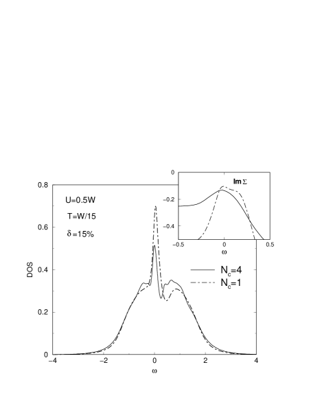
Figure 6: Local density of states for the 15% doped 1x1 ($N_{c}=1$) and 2x2 ($N_{c}=4$) cluster at fixed temperature $T=W/15$ and interaction $U=0.5W$. Inset: Imaginary part of the corresponding self energies in a narrow region around $\omega=0$.

Fig. 6 shows the density of states for both the 1x1 and 2x2 clusters for a doping of $\delta=15\%$. Both spectra display qualitatively similar features, namely the typical Hubbard bands and an enhanced density of states at the Fermi level $\omega=0$. For both cluster sizes the imaginary part of the corresponding self energies shows a parabolic minimum at the Fermi level as expected for a Fermi liquid, where $\left.-{\rm Im}\Sigma(\omega)\right|_{\omega\rightarrow 0}\propto\omega^{2}+\pi T^{2}$. In the case of the 2x2 cluster the self energy at the Fermi wave vector $\bar{\Sigma}(k_{F},\omega)$ is obtained from the above mentioned bilinear interpolation. Here $k_{F}$ lies along the diagonal from $(0,0)$ to $(\pi,\pi)$; however, for this set of parameters the self energy on the Fermi surface is almost isotropic and does not change its qualitative behavior as a function of the wave vector on the Fermi surface. The influence of nonlocal short-ranged dynamical correlations is visible in the 2x2 cluster calculation only in a slightly enhanced scattering rate at the Fermi level and therefore in a slightly reduced density of states as compared to the 1x1 result. The additional structures on top of the Hubbard bands can be traced back to the complex multiplet structure of the cluster. However, the qualitative physics remains unchanged by increasing the cluster size. This observation is consistent with the fact that at such strong doping antiferromagnetic fluctuations have practically died out and should thus show no significant influence on the physics of the system. The appearance of the quasi-particle resonance at low enough temperatures is well known in the case of the 1x1 cluster (DMFA): There it was shown that the evolution of this quasi-particle resonance with decreasing temperature is accompanied by a reduction of the effective local magnetic moment jarrell92 ; AdvPhy . This interplay of both effects is a fingerprint of the Kondo effect occurring in the single impurity Anderson model, which underlies the DMFA. Our results thus suggest that for the lattice system the physics is quite similar and the quasi-particle resonance at the Fermi level reflects Kondo like physics. It is important to note that this means that the Kondo like behavior in the Hubbard model is, at least for moderately to strongly doped systems, a real feature of the model and not an artifact of the limit of large dimensions.

For weakly doped or half filled systems, short-ranged antiferromagnetic spin fluctuations will be present and strong even at temperatures well above a magnetic transition. One thus expects that physics of the system will be strongly influenced and may even develop non-Fermi-liquid-like behavior.

Figure 7: Local density of states for the 1x1 ($N_{c}=1$) and 2x2 ($N_{c}=4$) cluster at fixed temperature $T=W/15$, interaction $U=0.5W$ and half filling. Inset: Imaginary part of the corresponding self energies in a narrow region around $\omega=0$.

Since these fluctuations will be strongest in the extreme case of half filling, we will consider this case next. Fig. 7 shows the results for both cluster sizes with the same parameters as in Fig. 6 but at half filling. Whereas the 1x1 cluster result displays the same features as in the doped case - enhanced density of states at the Fermi level accompanied by a parabolic minimum in the imaginary part of the self energy - the spectrum of the 2x2 cluster calculation is completely different from the doped case: Instead of forming a quasi-particle resonance as in the DMFA, the density of states develops a pseudogap at zero frequency and the corresponding imaginary part of the self energy which is again almost isotropic displays a strongly enhanced scattering rate at the Fermi energy. This surprising and interesting behavior has two possible explanations. The first and physically most appealing one is that short-ranged antiferromagnetic fluctuations do indeed drive the system from a Fermi liquid into a non Fermi liquid at temperatures high compared to the Néel temperature. Note that the underlying mechanism is very similar to the interpretation of the pseudogaps observed in the high-$T_{c}$ compounds well above $T_{c}$. The second interpretation is that the nonlocal corrections yield a reduction in the critical value $U_{c}$ at which the Mott-Hubbard metal-insulator transition occurs.

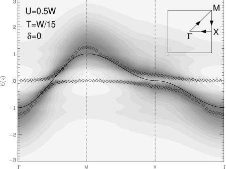
Figure 8: Contour-plot of the spectral density for the 2x2 cluster calculation along the main symmetry directions as indicated in the inset for the same parameters as in Fig. 7. The dark color marks regions with high spectral density. The open symbols indicate the maxima of the spectral function. The solid line marks the dispersion for the noninteracting system.

A contour-plot of the spectral density $A({\bf k},\omega)$ obtained with the bilinear interpolation scheme discussed earlier along the main symmetry directions in the Brillouin zone is shown in Fig. 8. The dark shading marks regions with high spectral density. The open symbols in Fig. 8 represent the positions of the most pronounced local maxima of $A({\bf k},\omega)$ and can be viewed as effective band structure of the 2D Hubbard model for the set of parameters under consideration. Compared to the bandstructure of the noninteracting system (illustrated by the solid line) the interactions have various effects on the spectrum. The band of the noninteracting system splits into two separated bands above and below the Fermi-energy. Note that the spectral density corresponding to the nearly dispersionless features of the two bands is very low and comparatively broad in the regions without states of the noninteracting system. We again notice the opening of the pseudogap at the Fermi-energy which is most pronounced at the X-point $(\pi/2,\pi/2)$. But in addition to these effects we now can resolve additional incoherent background structures at the points $\Gamma$ at $E(k)\approx 1$ and M at $E(k)\approx-1$. These additional states are just shifted by the wave vector ${\bf Q}=(\pi,\pi)$ with respect to the main bandstructure.

Figure 9: Spectral density at the points $\Gamma$ and M for the same parameters as in Fig. 7 and 8. Note the occurrence of shadow structures with small spectral weight in addition to the main structures.

In order to better resolve these structures we show the corresponding spectral density at the points $\Gamma$ and M in Fig. 9. In addition to the main structure at $\omega<0$ for the point $\Gamma$ ($\omega>0$ for M) we notice satellites at $\omega>0$ for $\Gamma$ ($\omega<0$ for M) with small spectral weight. These new states are absent in the non-interacting system as well as in the DMFA and result from the nonlocal antiferromagnetic correlations. Even in the paramagnetic phase the short-ranged antiferromagnetic spin fluctuations are sufficient to produce this indication of the ordered phase. Such a precursor effect of the antiferromagnetic long range order can for example be seen in the cuprates shadow in Fermi-surface measurements. The observation of these spin-fluctuation-induced shadow states accompanied by an opening of a pseudogap strongly supports the first suggested scenario of the antiferromagnetic spin fluctuations driving the system to a non Fermi liquid.

To gain more insight in the nature of the pseudogap and elucidate the physics of the observed non Fermi liquid behavior we added a next nearest neighbor hopping $t^{\prime}$ to the hopping integrals $t_{ij}$ in the Hamiltonian (1). The dispersion then becomes $\epsilon_{\bf k}=-2t(\cos k_{x}+\cos k_{y})+4t^{\prime}\cos k_{x}\cos k_{y}$ and the Fermi surface is no longer nested because $\epsilon_{{\bf k}+{\bf Q}}\neq-\epsilon_{\bf k}$ for the nesting vector ${\bf Q}=(\pi,\pi)$. By including $t^{\prime}$ we can thus frustrate the lattice and gradually suppress antiferromagnetic spin fluctuations. On the other hand, since we keep the non-interacting bandwidth $W$ and therefore the ratio $U/W$ fixed when including the $t^{\prime}$, we do not expecte this change to affect the Mott-Hubbard transition very drastically. Therefore, if the pseudogap is a precursor of the Mott-Hubbard transition we do not expect it to be influenced dramatically when we increase $t^{\prime}$.

Figure 10: Local density of states for the 2x2 ($N_{c}=4$) cluster at fixed temperature $T=W/15$, interaction $U=0.5W$ and half filling for various values of the next nearest neighbor hopping integral $t^{\prime}$.

Fig. 10 shows the behavior of the local density of states as the next nearest neighbor hopping $t^{\prime}$ and therefore the lattice frustration increases. First note that we lose particle hole symmetry for $t^{\prime}\neq 0$ because the bare density of states is no longer particle hole symmetric. Obviously, as $t^{\prime}$ increases, the pronounced pseudogap for $t^{\prime}=0$ gets gradually reduced. However, even for the maximum value $|t^{\prime}|=|t|$ we still see a small dip at zero frequency, which possibly can be attributed to the fact that even for a completely frustrated system extreme short-ranged fluctuations will be present, which are however strongly reduced in magnitude as compared to the nested situation. We thus conclude that indeed the nonlocal, short-ranged antiferromagnetic spin correlations are responsible for the development of the pseudogap at the Fermi energy in the Hubbard model with $t^{\prime}=0$ at half filling, which in fact must be viewed as precursor of an antiferromagnetically ordered state at much lower temperatures. One highly interesting question to be addressed in our future work will be of what precise nature this non Fermi liquid state is and how it might be related to several phenomenological scenarios proposed for the two-dimensional Hubbard model.

As a further illustration of the ability of the DCA to include nonlocal correlations, we show results for a larger interaction strength $U=1.3W$ and lower temperature $T=W/30$. For the hopping integrals we chose $t=0.25$ and $t^{\prime}=-0.35t$ to immitate the measured Fermisurface of underdoped cuprates in the non-interacting system preformed0 ; schmalian . Since we expect the spectra to display sharp features at this low temperature, we refrain from performing a bilinear interpolation of the self-energy and show results for the coarse grained spectra only. Fig. 11 shows the coarse grained spectral functions $\bar{A}({\bf K},\omega)=-1/\pi\Im m\bar{G}({\bf K},\omega)$ at ${\bf K}=(0,0)$ and ${\bf K}=(\pi,0)$ for a doping $\delta=10\%$ and temperature $T=W/30$ in a narrow region around the Fermienergy.

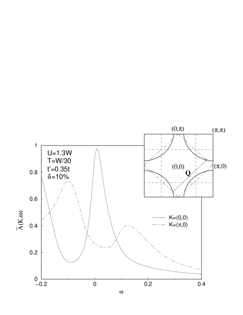
Figure 11: Coarse grained spectral function of the cells around ${\bf K}=(0,0)$ and $(\pi,0)$ for $N_{c}=4$ and a doping concentration $\delta=10\%$, temperature $T=W/30$ and hopping integrals $t=0.25$ and $t^{\prime}=-0.35t$. The inset shows the Fermisurface of the corresponding non-interacting system (solid line), the nested ${\bf k}$-points (dot-dashed line) and the boundaries of the coarse graining cells (dashed lines).

First we notice a strong anisotropy in the coarse grained functions. For the states located in the cell around ${\bf K}=(0,0)$ the spectrum is peaked at the Fermi-energy and only slightly broadened due to the finite temperature as characteristic for a Fermi liquid. The situation is completely different in the cell around the point $(\pi,0)$. All the spectral weight is transfered to broad features at higher energies, which represents the incoherent part of the spectrum. Therefore a pseudogap opens at the Fermi-energy.

Our results are qualitatively in agreement with calculations schmalian for the spin fluctuation model, in which the magnetic interaction between the quasiparticles is held responsible for the anomalous normal state properties of the cuprates. This method provides a direct explanation for the anisotropic behavior of the spectral density. Within this approach the electron-electron interaction is mediated by an imperially determined dynamical spin susceptibility. Since this susceptibility is strongly peaked at the antiferromagnetic wave vector ${\bf Q}=(\pi,\pi)$, one has to distinguish two different regions of the Fermi surface: Quasiparticles in regions of the Fermisurface which can be connected by the wave vector $\bf Q$ are called hot quasiparticles because they feel the full effects of the spin fluctuation induced interaction because of nesting. This is illustrated in the inset of Fig. 11, which displays the corresponding non-interacting Fermisurface for the chosen parameters. One can notice that the hot quasiparticles are located in the cell around $(\pi,0)$ and therefore represented by the coarse grained spectral function at ${\bf K}=(\pi,0)$. On the other hand the cold quasiparticles located along the diagonal couple only weakly to the spin excitations, since the Fermisurface in this region is not nested. This part of the Femisurface falls in the cell around ${\bf K}=(0,0)$ and therefore the spectrum in this cell displays Fermi-liquid like behavior. The spectrum around $(\pi,0)$ on the other hand gets strongly renormalized due to the strong coupling to the spin excitations. This phenomenological picture provides a direct explanation of our results qualitatively consistent with the calculations for the spin fluctuation model.

Calculations for larger doping ($\delta=20\%$) (not shown here) show that this effect of the anisotropic behavior of the spectrum and the opening of the pseudogap in the hot regions disappears. This observation can also be understood within the picture of the spin fluctuation induced correlations, since the antiferromagnetic spin fluctuations become strongly suppressed upon doping.

7 Conclusion

We motivated the recently introduced Dynamical cluster approximation (DCA) by its microscopic definition based on a choice for the Laue function. It partially restores the momentum conservation at the internal vertices which was relinquished in the Dynamical Mean Field Approximation (DMFA). The resulting theory maps the lattice problem onto a self-consistently embedded periodic cluster of size $N_{c}$. The DCA is a fully causal and systematic approximation to the full lattice problem with corrections ${\cal{O}}(1/N_{c})$ in two dimensions. We develop a Non Crossing Approximation (NCA) to solve the effective cluster problem which is a systematic $\Phi$-derivable approximation to the cluster problem with corrections ${\cal{O}}(1/N_{c}^{3})$.

We applied our DCA-NCA formalism to the Hubbard model on a square lattice and calculated the single-particle properties when $N_{c}=1$ and $N_{c}=4$. For a highly doped system, with $\delta=15\%$ and a Hubbard $U$ of half the bare bandwidth, nonlocal correlations present when $N_{c}=4$ turned out to be unimportant and both cluster sizes yield qualitatively similar results with an enhanced density of states and a minimum in the scattering rate at the Fermi energy. Thus, independent of the cluster size, the highly doped system showed Fermi liquid character. However, as the doping decreases, the non-local correlations become far more important, and the half-filled system displays strikingly different results for the two cluster sizes. Whereas the $N_{c}=1$ cluster result still displays Fermi liquid like behavior, the $N_{c}=4$ cluster calculation shows the opening of a pseudogap in the density of states and therefore non Fermi liquid character. Calculations with a next nearest neighbor hopping $t^{\prime}$ show evidence that this pseudogap is due to antiferromagnetic spin correlations and therefore a single particle precursor of the antiferromagnetic phase transition. The pseudogap persists upon weak doping in qualitative agreement with the spin fluctuation model for the cuprates.

Hence our calculations have shown that for the weakly doped system, nonlocal correlations play an important role on the single particle properties and change the character of the system from a Fermi liquid to a non Fermi liquid. These non-local features are missing in the DMFA spectra, but appear in the DCA spectra as soon as the cluster size exceeds one.

Acknowledgements: It is a pleasure to acknowledge discussions with P.G.J. van Dongen, D. Hess, M. Hettler, H.R. Krishnamurthy, E. Müller-Hartmann, and F.-C. Zhang. This work was supported by NSF grants DMR-9704021, DMR-9357199, the Graduiertenkolleg “Komplexität in Festkörpern” and the NATO Collaborative Research Grant CRG970311. Computer support was provided by the Ohio Supercomputer Center and the Leibnitz-Rechenzentrum, Munich.

Appendix A On the analyticity of $\Gamma({\bf K},z)$

The following proof of the analyticity of $\Gamma({\bf K},z)$ is based on the derivation of an analytic expression for the cluster Green’s function

$$\bar{G}({\bf K},z)=\frac{N_{c}}{N}\sum\limits_{{\bf k}^{\prime}}\frac{1}{z+\mu-\epsilon_{{\bf K}+{\bf k}^{\prime}}-\Sigma_{c}({\bf K},z)}\;\;.$$

The self-energy function $\Sigma_{c}({\bf K},z)$ is assumed to be analytic in the upper and lower half of the complex plane with ${\rm sign}(\Im m\Sigma_{c}({\bf K},z))=-{\rm sign}\Im m(z)$. Our proof employs standard methods of projection technique grosso ; magnus . To this end we abbreviate $\xi_{\bf K}=z+\mu-\Sigma_{c}({\bf K},z)$, $\Im m(\xi_{\bf K})>0$ and introduce a $N/N_{c}$ dimensional set of linearly independent vectors $|{{\bf k}^{\prime}}\rangle$ and a linear hermitian operator ${\cal H}_{\bf K}$ satisfying ${\cal H}_{\bf K}|{{\bf k}^{\prime}}\rangle=\epsilon_{{\bf K}+{\bf k}^{\prime}}|{{\bf k}^{\prime}}\rangle$ and $\sum\limits_{{\bf k}^{\prime}}|{{\bf k}^{\prime}}\rangle\langle{{\bf k}^{\prime}}|=1$. There obviously exists another vector $|{f_{0}}\rangle$ with $\langle{{\bf k}^{\prime}}|f_{0}\rangle=\sqrt{N_{c}/N}$ for all ${\bf k}^{\prime}$. With these conventions we may write

$$\bar{G}({\bf K},z)=\langle{f_{0}}|\frac{1}{\xi_{\bf K}-{\cal H}_{\bf K}}|{f_{0}}\rangle\;\;.$$

The resolvent operator may be trivially rewritten as

$$\frac{1}{\xi_{\bf K}-{\cal H}_{\bf K}}=\frac{1}{\xi_{\bf K}}+\frac{1}{\xi_{\bf K}}{\cal H}_{\bf K}\frac{1}{\xi_{\bf K}-{\cal H}_{\bf K}}$$

and thus

$$\langle{f_{0}}|\frac{1}{\xi_{\bf K}-{\cal H}_{\bf K}}|{f_{0}}\rangle=\frac{1}{\xi_{\bf K}}+\frac{1}{\xi_{\bf K}}\langle{f_{0}}|{\cal H}_{\bf K}\frac{1}{\xi_{\bf K}-{\cal H}_{\bf K}}|{f_{0}}\rangle\;\;,$$

where we made use of $\langle{f_{0}}|{f_{0}}\rangle=1$. We now define two projection operators $P=|{f_{0}}\rangle\langle{f_{0}}|$ and $Q=1-P$ and insert $1=P+Q$ after ${\cal H}_{\bf K}$ in the second term, leading to

$$\langle{f_{0}}|\frac{1}{\xi_{\bf K}-{\cal H}_{\bf K}}|{f_{0}}\rangle=\begin{array}[t]{l}\displaystyle\frac{1}{\xi_{\bf K}}+\frac{1}{\xi_{\bf K}}\langle{f_{0}}|{\cal H}_{\bf K}|{f_{0}}\rangle\langle{f_{0}}|\frac{1}{\xi_{\bf K}-{\cal H}_{\bf K}}|{f_{0}}\rangle\\[14.22636pt] \displaystyle+\frac{1}{\xi_{\bf K}}\langle{f_{0}}|{\cal H}_{\bf K}Q\frac{1}{\xi_{\bf K}-{\cal H}_{\bf K}}|{f_{0}}\rangle\;\;.\end{array}$$

Since furthermore

$$\frac{1}{\xi_{\bf K}-{\cal H}_{\bf K}}=\begin{array}[t]{l}\displaystyle\frac{1}{\xi_{\bf K}-{\cal H}_{\bf K}Q-{\cal H}_{\bf K}P}=\displaystyle\frac{1}{\xi_{\bf K}-{\cal H}_{\bf K}Q}+\\[14.22636pt] \displaystyle\frac{1}{\xi_{\bf K}-{\cal H}_{\bf K}Q}{\cal H}_{\bf K}P\frac{1}{\xi_{\bf K}-{\cal H}_{\bf K}}\end{array}$$

and due to $Q|{f_{0}}\rangle=0$

$$Q\frac{1}{\xi_{\bf K}-{\cal H}_{\bf K}Q}|{f_{0}}\rangle=0$$

we finally obtain

$$\begin{array}[t]{l}\displaystyle\langle{f_{0}}|\frac{1}{\xi_{\bf K}-{\cal H}_{\bf K}}|{f_{0}}\rangle=\displaystyle\frac{1}{\xi_{\bf K}}+\frac{1}{\xi_{\bf K}}\langle{f_{0}}|{\cal H}_{\bf K}|{f_{0}}\rangle\langle{f_{0}}|\frac{1}{\xi_{\bf K}-{\cal H}_{\bf K}}|{f_{0}}\rangle\\[14.22636pt] \displaystyle+\frac{1}{\xi_{\bf K}}\langle{f_{0}}|{\cal H}_{\bf K}Q\frac{1}{\xi_{\bf K}-{\cal H}_{\bf K}Q}{\cal H}_{\bf K}|{f_{0}}\rangle\langle{f_{0}}|\frac{1}{\xi_{\bf K}-{\cal H}_{\bf K}}|{f_{0}}\rangle\;\;.\end{array}$$

With $Q^{2}=Q$ we may rewrite

$${\cal H}_{\bf K}Q\frac{1}{\xi_{\bf K}-{\cal H}_{\bf K}Q}{\cal H}_{\bf K}={\cal H}_{\bf K}Q\frac{1}{\xi_{\bf K}-Q{\cal H}_{\bf K}Q}Q{\cal H}_{\bf K}\;\;.$$

With the abbreviations

$$\Gamma({\bf K},z)=\langle{f_{0}}|{\cal H}_{\bf K}Q\frac{1}{\xi_{\bf K}-Q{\cal H}_{\bf K}Q}Q{\cal H}_{\bf K}|{f_{0}}\rangle$$

and

$$\bar{\epsilon}_{\bf K}=\langle{f_{0}}|{\cal H}_{\bf K}|{f_{0}}\rangle=\frac{N_{c}}{N}\sum\limits_{{\bf k}^{\prime}}\epsilon_{{\bf K}+{\bf k}^{\prime}}$$

the final result is

$$\bar{G}({\bf K},z)=\frac{1}{\xi_{\bf K}-\bar{\epsilon}_{\bf K}-\Gamma({\bf K},z)}\;\;.$$ (26)

Note however that the averaging procedure replaces the kinetic energy of the lattice $\epsilon_{\bf k}$ by a quantity coarse grained onto the cluster.

We are now left with the proof that ${\rm sign}\Im m(\Gamma({\bf K},z))=-{\rm sign}\Im m(z)$ is fulfilled. This however can easily be done by repeating the above step for the new vector $|{f_{1}}\rangle=Q{\cal H}_{\bf K}|{f_{0}}\rangle={\cal H}_{\bf K}|{f_{0}}\rangle-\bar{\epsilon}_{\bf K}|{f_{0}}\rangle$, $\langle{f_{0}}|{f_{1}}\rangle=0$, appearing in the definition of $\Gamma({\bf K},z)$. Note that this is simply the first step in a Schmitt-Graham procedure to generate an orthogonal set of vectors. With $\tilde{\cal H}_{\bf K}=Q{\cal H}_{\bf K}Q$ it follows

$$\Gamma({\bf K},z)=\frac{b_{0}^{2}}{\xi_{\bf K}-a_{1}-\bar{\Gamma}({\bf K},z)}\;\;,$$ (27)

where

$$\begin{array}[]{l}\displaystyle b_{0}^{2}=\frac{\langle{f_{1}}|{f_{1}}\rangle}{\langle{f_{0}}|{f_{0}}\rangle}\geq 0\\[14.22636pt] \displaystyle a_{1}=\frac{\langle{f_{1}}|{\cal H}_{\bf K}|{f_{1}}\rangle}{\langle{f_{1}}|{f_{1}}\rangle}\\[14.22636pt] \displaystyle\bar{\Gamma}({\bf K},z)=\frac{1}{\langle{f_{1}}|{f_{1}}\rangle}\langle{f_{1}}|\tilde{\cal H}_{\bf K}\tilde{Q}\frac{1}{\xi_{\bf K}-\tilde{Q}\tilde{\cal H}_{\bf K}\tilde{Q}}\tilde{Q}\tilde{\cal H}_{\bf K}|{f_{1}}\rangle\;\;,\end{array}$$

where $\tilde{Q}$ now projects onto the subspace orthogonal to $|{f_{0}}\rangle$ and $|{f_{1}}\rangle$. It is clear from the above result that this procedure can be repeated, leading to a sequence of mutually orthogonal vectors $|{f_{n}}\rangle={\cal H}_{\bf K}|{f_{n-1}}\rangle-a_{n-1}|{f_{n-1}}\rangle-b_{n-2}^{2}|{f_{n-2}}\rangle$ and a continued fraction representation of $\bar{G}({\bf K},z)$ with coefficients

$$\begin{array}[]{l}\displaystyle b_{n-1}^{2}=\frac{\langle{f_{n}}|{f_{n}}\rangle}{\langle{f_{n-1}}|{f_{n-1}}\rangle}\geq 0\\[14.22636pt] \displaystyle a_{n}=\frac{\langle{f_{n}}|{\cal H}_{\bf K}|{f_{n}}\rangle}{\langle{f_{n}}|{f_{n}}\rangle}\end{array}$$

for $n\geq 1$. It is important to emphasize that the resulting coefficients $b_{n-1}^{2}$ are non-negative by construction. This however immediately leads to the desired relation ${\rm sign}\Im m(\Gamma({\bf K},z))=-{\rm sign}\Im m(z)$ and hence to the causality of $\Gamma({\bf K},z)$.

Appendix B Proof of $\Gamma({\bf K})\sim{\cal O}(1/N_{c})$

The following proof is based on the definitions (10,11) of the coarse grained Green function $\bar{G}$. With $g^{-1}({\bf K})=\omega-\bar{\epsilon}_{\bf K}-\bar{\Sigma}({\bf K})$ we can rewrite $\bar{G}$ in the form

$$\bar{G}({\bf K}) = \frac{N_{c}}{N}\sum_{\tilde{\bf k}}G({\bf K}+\tilde{\bf k})$$ (28)

$$= \frac{1}{g^{-1}({\bf K})-\Gamma({\bf K})}\quad\mbox{,}$$

where we dropped the frequency argument for convenience. By defining

$$t_{{\bf K}+\tilde{\bf k}}=\epsilon_{{\bf K}+\tilde{\bf k}}-\bar{\epsilon}_{\bf K}\quad\mbox{,}$$ (29)

such that $N_{c}/N\sum_{\tilde{\bf k}}t_{{\bf K}+\tilde{\bf k}}=0$ we can make use of the exact relation

$$G({\bf K}+\tilde{\bf k})=g({\bf K})+g({\bf K})t_{{\bf K}+\tilde{\bf k}}G({\bf K}+\tilde{\bf k})\quad\mbox{.}$$ (30)

By inserting (30) in (28) it is straightforward to show that $\Gamma({\bf K})$ is given by

$$\Gamma({\bf K})=\frac{\displaystyle\frac{N_{c}}{N}\sum_{\tilde{\bf k}}t^{2}_{{\bf K}+\tilde{\bf k}}G({\bf K}+\tilde{\bf k})}{\displaystyle 1+\frac{N_{c}}{N}\sum_{\tilde{\bf k}}t_{{\bf K}+\tilde{\bf k}}G({\bf K}+\tilde{\bf k})}\quad\mbox{.}$$ (31)

By performing a Taylor series expansion of $t_{{\bf K}+\tilde{\bf k}}$ around the cluster points $\bf K$ it can be seen that $t_{{\bf K}+\tilde{\bf k}}$ is of order ${\cal O}(\Delta k)$, where $\Delta k=2\pi/N_{c}^{1/D}$. Therefore we see from Eq. 31 that $\Gamma({\bf K})$ is of order ${\cal O}((\Delta k)^{2})$ and for two dimensions we finally get the result

$$\Gamma({\bf K})\sim{\cal O}(1/N_{c})\quad\mbox{.}$$ (32)

References

- (1) N. Grewe and F. Steglich, Handbook on the Physics and Chemistry of Rare Earths, Eds. K.A. Gschneidner, Jr. and L.L. Eyring (Elsevier, Amsterdam, 1991) Vol. 14, P. 343; D. W. Hess, P. S. Riseborough, J. L. Smith, Encyclopedia of Applied Physics Eds. G. L. Trigg (VCH Publishers Inc., NY), Vol.7 (1993) p. 435.
- (2) J.G. Bednorz and K.A. Müller, Z. Phys. 64, 189 (1986)
- (3) E.H. Lieb and F.Y. Wu, Phys. Rev. Lett., 20, 1445 (1968)
- (4) E. Dagotto, Correlated Fermions in high-temperature superconductors, Rev. Mod. Phys. 66, 763 (1994)
- (5) U. Brandt and C. Mielsch, Z. Phys. B75, 365 (1989)
- (6) V. Janiš, Z. Phys. B83, 227 (1991)
- (7) M. Jarrell, Phys. Rev. Lett. 69, 168 (1992)
- (8) A. Georges and G. Kotliar, Phys. Rev. B45, 6479 (1992)
- (9) M. Jarrell and Th. Pruschke, Z. Phys. B, 90, 187-194 (1993).
- (10) Th. Pruschke, Th. Obermeier, J. Keller and M. Jarrell, Physica B 223 & 224, 611(1996).
- (11) P. Aebi et al., Phys. Rev. Lett. 72 2757 (1994)
- (12) H. Ding et al., Nature (London) 382, 51 (1996)
- (13) R.E. Walsted and W.W. Warren, Appl. Magn. Reson. 3, 469 (1992)
- (14) J. Loram et al., Phys. Rev. Lett., 71, 1740 (1993)
- (15) J.L. Tallon et al., Phys. Rev. Lett., 75 4414 (1995)
- (16) P.G.J. van Dongen, Phys. Rev. B 50, 14016 (1994). It follows immediately from Eq. A9 therein, that the spectral weight has an acausal part of order [P.G.J. van Dongen, private communication]
- (17) A. Schiller and K. Ingersent, Phys. Rev. Lett. 75, 113, (1995)
- (18) Th. Obermeier, Th. Pruschke, J. Keller, Physica B, 230-232, 892 (1997)
- (19) Tran Minh-Tien, Phys. Rev. B 58, 15965 (1998)
- (20) M.H. Hettler, A.N. Tahvildar-Zadeh and M. Jarrell, Phys. Rev. B 58 7475
- (21) M.H. Hettler et al., preprint cond-mat/9903273
- (22) Th. Pruschke, D.L. Cox, M. Jarrell, Phys. Rev. B 47 3553 (1993)
- (23) Th. Pruschke, Q. Qin, Th. Obermeier and J. Keller, J. of Phys. -Condens. Matter 8, 3161 (1996)
- (24) Th. Obermeier, Th. Pruschke and J. Keller, Phys. Rev. B 56, 8479 (1997)
- (25) J. Schmalian, P. Lombardo, M. Avignon, K.H. Bennemann, Physica B 223-224, 602 (1995); P. Lombardo, M. Avignon, J. Schmalian, K.H. Bennemann, Phys. Rev. B 54, 5317 (1996)
- (26) Th. Maier, M.B. Zölfl, Th. Pruschke and J. Keller, Eur. Phys. J. B 7, 377 (1999)
- (27) W. Metzner and D. Vollhardt, Phys. Rev. Lett. 62, 324 (1989)
- (28) E. Müller-Hartmann, Z. Phys. B, 74, 507–512 (1989)
- (29) H. Keiter, J.C. Kimball, Intern. J. Magnetism 1, 233 (1971)
- (30) Th. Pruschke and N. Grewe, Z. Phys. B 74, 439 (1998)
- (31) K. Fischer, Ph.D. thesis at the Max-Planck-Institut für Komplexe Systeme, Dresden, 1995; K. Fischer, Phys. Ref. B, 13575 (1997)
- (32) Th. Pruschke, M. Jarrell and J.K. Freericks, Adv. in Phys. 42, 187 (1995)
- (33) It is possible that an exact-diagonalization based generalization of the approach presented here will make larger clusters more tractable. The first step in our NCA approach involves diagonalizing the molecular cluster. If this was the limiting step in our technique, we should be able to treat clusters as large as those presently studied by exact diagonalization. However, the remaining numerical task of calculating the coupled equations (22) and (23) self-consistently is necessary for the NCA to be derivable, but it becomes formidable as the cluster size increases. The -derivability is important since it guarantees that our results will be consistent at the one and two-particle level. If we were to relax this condition, and neglect the higher-order, and higher, non-crossing diagrams by using bare resolvents in (23), then we could treat significantly larger clusters and the approximation would still be correct up to .
- (34) J. Schmalian et al., preprint cond-mat/9804129.
- (35) G. Grosso and G. Pastori Parravicini, in Memory Function Approaches to Stochastic Problems in Condensed Matter, edited by M.W. Evans, P. Grigolini and G. Pastori Parravicini, Advances in Chemical Physics, Vol. 62(Wiley, New York 1985), p. 133.
- (36) A. Magnus in The Recursion Method and its Applications, edited by D.G. Pettifor. D.L. Weaire, Springer Series in Solid State Sciences Vol. 58 (Springer Berlin 1985).