Calculations of exchange interaction in impurity band of two-dimensional semiconductors with out of plane impurities

Abstract

We calculate the singlet-triplet splitting for a couple of two-dimensional electrons in the potential of two positively charged impurities which are located out of plane. We consider different relations between vertical distances of impurities $h_{1}$ and $h_{2}$ and their lateral distance $R$. Such a system has never been studied in atomic physics but the methods, worked out for regular two-atomic molecules and helium atom, have been found to be useful. Analytical expressions for several different limiting configurations of impurities are obtained an interpolated formula for intermediate range of parameters is proposed. The $R$-dependence of the splitting is shown to become weaker with increasing $h_{1},h_{2}$.

I Introduction

Two-particle exchange interaction is the main mechanism of the spin-spin interaction in the impurity band of semiconductors. The recent experiments[2, 3] on the metallic phase in two-dimensional system show that a magnetic field parallel to the plane of the two-dimensional electron gas can destroy this phase. This suggests that the spin interaction plays an important role in the formation of the metallic state. The study of low-dimensional spin systems is usually based on the Heisenberg Hamiltonian $\sum_{\langle ik\rangle}J_{ik}{\bf s_{i}\cdot s_{k}}$, where ${\bf s}$ is the spin 1/2 operator, and $i,k$ denote different spins. Thus, the knowledge of the exchange constants $J_{ik}$, which are equal to half of the singlet-triplet energy splitting for two electrons located at different sites is very important.

In our previous paper[4] we have calculated these parameters and have obtained analytical expression for the ground state and excited states of the Heisenberg Hamiltonian at small impurity density. We assumed, however that impurities are located in the same plane as electron gas. This is not the case in usual semiconductor structures, where impurities are separated from electrons by the so-called spacer layer and residual impurities are also out of plane containing electron gas. In this paper we concentrate on the problem of spin splitting in the system of two electrons bound to the Coulomb centers which are located outside the plain.

Fig. 1. illustrates the general geometry of the problem.

FIG. 1.: General geometry of the problem

The total Hamiltonian of our artificial molecule is

$$\hat{H}=-\frac{\Delta_{1}}{2}-\frac{\Delta_{2}}{2}-\sum_{j,i=1}^{2}\frac{1}{\sqrt{h_{j}^{2}+(x_{i}-(-1)^{j}a)^{2}+y_{i}^{2}}}+\frac{1}{r_{12}}+\frac{1}{\sqrt{R^{2}+(h_{2}-h_{1})^{2}}}$$ (1)

Hereafter we use effective atomic units (a.u.) which means that all distances are measured in units of the effective Bohr radius $a_{B}=\hbar^{2}\epsilon/m^{*}e^{2}$, and energies in units of $m^{*}e^{4}/\hbar^{2}\epsilon^{2}$, where $m^{*}$ is the effective mass of the electron, and $\epsilon$ is the dielectric constant. The projection of the distance between impurities onto the plane of electron gas is $R\equiv 2a$ and the $x$-coordinates of the impurities are $\pm a$.

Three parameters, which determine the behavior of the system, are $h_{1},\ h_{2},$ and $R$. Of course, there is no analytical solution for $J(h_{1},h_{2},R)$ for the whole range of parameters. In the present work we investigate the different analytical limits of the Hamiltonian (1) and present an interpolated formula, which connects these limits.

If $h_{1}\sim h_{2}\sim h$ the method of the calculations is primarily determined by the ratio $h/R$. This can be understood by looking at the single-particle unperturbed potential (see Fig. 2).

$$V_{1}(x,y)=-\frac{1}{\sqrt{h_{1}^{2}+(x+a)^{2}+y^{2}}}-\frac{1}{\sqrt{h_{2}^{2}+(x-a)^{2}+y^{2}}}.$$ (2)

FIG. 2.: The cross section $y=0$ of the single-particle potential $V_{1}(x,y)$. The dotted line is the Helium-like atom ($h_{1},h_{2}>R$), and the solid line is the Hydrogen-like molecule ($h_{1},h_{2}<R$).

Function $V_{1}(x,y)$ has either one or two minima. The transition from one case to another happens when a minimum near the origin changes for a maximum. For the case of equal heights $h_{1}=h_{2}=h$ the function $V_{1}(x,y)$ has one minimum if $h/R\geq 1/\sqrt{2}$.

The case $h_{1},h_{2}<R$ corresponds to a $2D$ Hydrogen-like molecule, when there are two well-separated minima. In this case the splitting is exponentially small and determined by the degree of overlapping of wave-functions in the classically forbidden under-barrier region (especially at $r_{1},r_{2}\approx 0$).

The opposite case $h_{1},h_{2}>R$ corresponds to a $2D$ Helium-like atom when only one minimum exists, and the interaction term $1/r_{12}$ should be taken into account from the very beginning.

If the difference between $h_{1}$ and $h_{2}$ is large enough then the electrons will spend most of their time in the potential well of the impurity closest to the plane. The potential $V_{1}(x,y)$ has one minimum in this case. Therefore this case corresponds to a perturbed “Helium” atom (or perturbed ion $H^{-}$).

The paper is organized as follows. In Section 2 we consider the case of a hydrogen-like molecule ($R>2h$). By making use of semiclassical methods we obtain analytical results for a pure two-dimensional hydrogen molecule ($h_{1},\ h_{2}=0,\ R\gg 1$)[4]. The perturbation theory results ($h_{1,2}\ll 1<R$) and the saddle point method ($1<h_{1,2}\ll R$) represent other analytical limits in this case. The details of the calculations are given in appendices A,B.

In Section 3 we discuss a helium-like atom ($h_{1,2}>R$). We start from the result for pure two-dimensional helium[4] ($R=h_{1,2}=0$) and calculate the perturbation theory corrections. The quadratic approximation is applied to the limit $h_{1,2}>R>1$. Section 4 is devoted to the interpolated formula, which connects the two different limits for the distance $R$ at fixed vertical coordinates of impurities $h_{1},h_{2}$. Our results are summarized in the Conclusion.

II Hydrogen-like molecule

A General formula, $R\gg 1$.

The exchange constant $J_{ik}$ is defined as one-half of the energy difference between the lowest two-particle energies for total spins $S=1$ and $S=0$:

$$2J = (E_{g}^{S=1}-E_{g}^{S=0})\ \equiv(E_{A}-E_{S}),\quad\mbox{ where }$$ (3)

$$\hat{H}\Psi_{S} = E_{S}\Psi_{S},$$ (4)

$$\hat{H}\Psi_{A} = E_{A}\Psi_{A}.$$ (5)

Here $\Psi_{S}$ and $\Psi_{A}$ denote the lowest symmetrical and antisymmetrical two-particle coordinate wave functions of the singlet and triplet states respectively. When $h_{1,2}<R$ and $R\gg 1$ the most appropriate method to determine the term splitting due to the spin-spin interaction is the Gor’kov-Pitaevskii method [5, 6, 7]. We apply it here to the two-dimensional electron system. In accordance with this approach we reduce the expression for $J$ to a surface integral over a hyperplane in the $4$-dimensional coordinate space. To this end, we multiply Eq. (4) by $\Psi_{A}$ and Eq. (5) by $\Psi_{S}$, take the difference between the results and calculate the integral over a part of the volume in the four dimensional configuration space of the electrons. We choose the integration volume as a region $x_{1}\leq x_{2}$. This is a four-dimensional volume to the left of the hyperplane $\Sigma$ determined by the equation $x_{1}=x_{2}$. Using the Hamiltonian (1) and Gauss’ theorem we obtain

$$(E_{S}-E_{A})\int\!\!\int_{\Omega}\Psi_{A}\Psi_{S}\,d{\bf r_{1}}\,d{\bf r_{2}}=\oint_{\sigma}(\Psi_{S}\nabla\Psi_{A}-\Psi_{A}\nabla\Psi_{S})\,{\bf d\sigma},$$ (6)

where $\sigma$ is a closed hypersurface, and $\Omega$ is the volume bounded by $\sigma$.

Now we introduce a combinations of the functions $\Psi_{1,2}=1/\sqrt{2}(\Psi_{S}\pm\Psi_{A})$. If the phases of $\Psi_{S,A}$ are properly chosen, the function $\Psi_{1}$ will be large only when electron 1 is near the left minimum and electron 2 is near the right minimum. The function $\Psi_{2}$, obtained by permuting ${\bf r_{1}}$ with ${\bf r_{2}}$, is localized almost entirely on the “far” side. A simple calculation gives

$$\int\!\!\int_{\Omega}\Psi_{S}\Psi_{A}\,d{\bf r_{1}}\,d{\bf r_{2}}=\frac{1}{2}\int\!\!\int_{\Omega}(\Psi_{1}^{2}-\Psi_{2}^{2})\,d{\bf r_{1}}\,d{\bf r_{2}}\approx 1/2.$$

Substituting the wave functions $\Psi_{1,2}$ into Eq. (6) we finally obtain that $(E_{S}-E_{A})$ can be expressed as the integral over the hyperplane $\Sigma$.

$$2J=-2\int\left[\Psi_{2}\frac{\partial\Psi_{1}}{\partial x_{1}}-\Psi_{1}\frac{\partial\Psi_{2}}{\partial x_{1}}\right]_{x_{1}=x_{2}}~{}dx_{2}~{}dy_{1}~{}dy_{2}.$$ (7)

Eq. (7) shows that the main contribution to the exchange constant is given by the region where the electrons are close to each other. Indeed, the $x$ coordinates of both electrons coincide ($x_{1}=x_{2}$), however, the $y$ coordinates may be different. In this case there are strong correlations between the positions of the electrons due to Coulomb repulsion. This means that we should go beyond the approximation where the two-particle wave function of the electrons is represented as a product of single-particle wave functions.

The details of the calculation of the wave functions $\Psi_{1,2}$ and the surface integral (7) are presented in the appendices A,B. The final result is:

$$2J(\alpha,\beta,R)=R^{\frac{2}{\alpha}+\frac{2}{\beta}-\frac{1}{\mu}}e^{-\mu R}\left[D\left(\alpha,\beta,R\right)+D\left(\beta,\alpha,R\right)\right],$$ (8)

where the function $D\left(\alpha,\beta,R\right)$ is determined by Eq. (B17). Here

$$\frac{\alpha^{2}}{2}=-E(h_{1}),\ \frac{\beta^{2}}{2}=-E(h_{2})$$

are “ionization energies” in the potential $1/\sqrt{r^{2}+h^{2}}$, and $\mu=\alpha+\beta$.

B Two-dimensional hydrogen molecule and perturbation theory for $h_{1},\ h_{2}\ll 1$

In the case $\alpha=\beta$ the function $D(\alpha,\alpha,R)$ is independent of $R$:

$$D_{0}(\alpha)\equiv 2\,D\left(\alpha,\alpha,R\right)=8\sqrt{\pi}A_{\alpha}^{4}\left(\frac{1}{4\alpha}\right)^{1/2\alpha}\Gamma\left(\frac{\alpha+1}{2\alpha}\right)\int_{0}^{1}\exp\left(-t/\alpha\right)(2-t)^{1/2\alpha}t^{3/2\alpha}\,dt.$$ (9)

Therefore for the case $h_{1}=h_{2}$

$$2J(\alpha,\alpha,R)=D_{0}(\alpha)R^{7/2\alpha}\exp(-2\alpha R)$$ (10)

Here $A_{\alpha}$ is the normalization constant for the single particle wave function in the potential $1/\sqrt{r^{2}+h^{2}}$ (see Appendix A).

The case $h=0$ corresponds to the two-dimensional hydrogen molecule. In accordance with Appendix A we substitute $\alpha=2$ and $A_{\alpha}=4/\sqrt{2\pi}$ in Eq. (10) and we obtain

$$2J(2,2,R)=30.413\,R^{7/4}\exp(-4R)$$ (11)

We can carry out further analytical estimates for small $h_{1,2}$. When $h$ is much smaller than the Bohr radius we take $A_{\alpha}$ from (A14), put it into Eq. (9) and obtain

$$D_{0}(\alpha)=\frac{2^{3/\alpha+1}\alpha^{4+7/2\alpha}}{\pi^{3/2}}\frac{\Gamma\left(1/2+1/2\alpha\right)}{\Gamma\left(2/\alpha\right)^{2}}\int_{0}^{1}\exp\left(-t/\alpha\right)\left(2-t\right)^{1/2\alpha}t^{3/2\alpha}\,dt$$ (12)

Function $D_{0}(\alpha)$ is a regular function near the point $\alpha=2$ (see Fig. 3). It can be expanded in a Taylor series:

$$D_{0}(\alpha)\approx 30.413\left(1+1.665(\alpha-2)+0.456(\alpha-2)^{2}+\ldots\right)$$ (13)

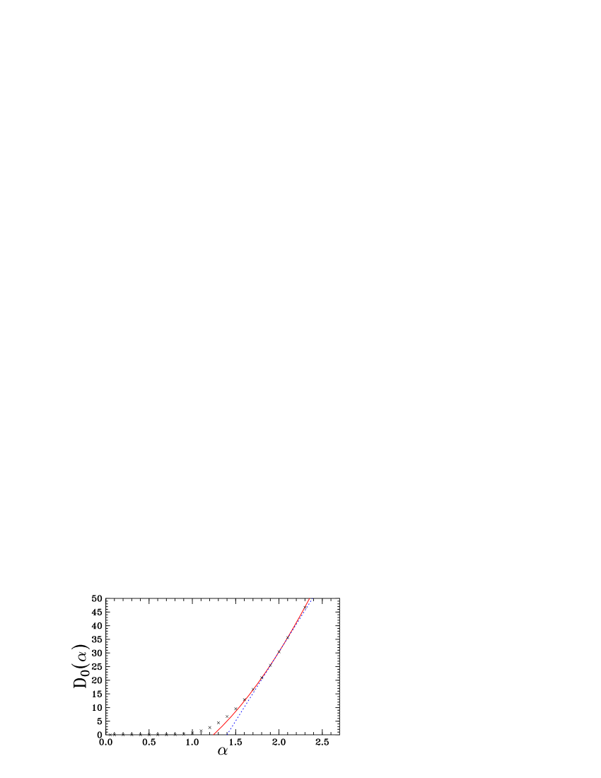
FIG. 3.: Exact (crosses), linear (dashed line) and quadratic (solid line) approximations for function $D_{0}(\alpha)$.

Taking into consideration that (see Appendix A)

$$\alpha\approx 2-\Delta_{E}/2$$

with

$$\Delta_{E}=16h\left(1+2h\ln(2h)\right),$$

finally we obtain

$$J(\alpha,\alpha,R)\approx J(2,2,R)\left[1-0.833\Delta_{E}\right]R^{\frac{7}{16}\Delta_{E}}\exp(\Delta_{E}R)\approx J(2,2,R)\left[1+\Delta_{E}(-0.833+R+\frac{7}{16}\ln(R))\right].$$ (14)

Thus, the splitting increases with $h$. Indeed, when the impurity centers go out of the plane the interaction between them and the electrons becomes smaller. Therefore, radii of bound single electron wave functions and overlapping increase.

When $h_{1}\neq h_{2}$ and $h_{1},h_{2}\ll 1$ the formula for $J$ should be rewritten in the form:

$$J(\alpha,\beta,R)\approx J(2,2,R)\left[1+\Delta_{E}(-d_{1}+R+7/16)+\delta_{E}d_{2}\right],$$ (15)

where

$$\Delta_{E},\delta_{E}=(\Delta_{E_{1}}\pm\Delta_{E_{2}})/2$$

and $d_{1},d_{2}$ are some coefficients which can be extracted from the expansion $D(\alpha,\beta,R)$ for small $h_{1,2}$.

C $1\ll h\ll R$. Saddle point method.

At $h\gg 1$, one can easily find that $E(h)\approx-1/h$ (See also Appendix A). Then $\alpha\approx\sqrt{2}/\sqrt{h}\ll 1$. and the integral in $D_{0}(\alpha)$ as well as the Gamma-function can be estimated by the saddle-point method:

$$\int_{0}^{1}e^{-t\lambda}(2-t)^{\lambda/2}t^{3\lambda/2}\,dt \approx \frac{e^{-\lambda/2}}{2}\sqrt{\frac{\pi}{\lambda}},$$ (16)

$$\Gamma(\lambda/2+1/2) \approx \sqrt{\pi(\lambda-1)}\left(\frac{\lambda-1}{2}\right)^{\frac{\lambda-1}{2}}\exp\left(-\frac{\lambda-1}{2}\right),$$ (17)

where $\lambda\equiv 1/\alpha$. Thus,

$$D_{0}(\alpha)\approx\frac{4}{\pi}\frac{1}{h^{3}}\frac{e^{-\lambda}}{\sqrt{\lambda}}\left[\frac{\lambda}{4}\right]^{\lambda/2}\sqrt{2\pi}\left[\frac{\lambda}{2}\right]^{\lambda/2}e^{-\lambda/2}=\sqrt{\frac{32\alpha}{\pi}}\frac{1}{h^{3}}\left[\alpha^{2}8e^{3}\right]^{-1/(2\alpha)},$$ (19)

and

$$2J(\alpha,\alpha,R)=\sqrt{\frac{32\alpha}{\pi}}\frac{1}{h^{3}}\left[\alpha^{2}8e^{3}\right]^{-1/(2\alpha)}R^{7/(2\alpha)}\exp(-2\alpha R),\qquad h\gg 1,R/h\gg 1.$$ (20)

III Helium-like atom

A Pure $2D$ Helium atom.

When two impurities are close to each other ($R\lesssim\sqrt{2}h$) there is only one minimum for the single-particle potential $V_{1}(x,y)$. Hence, the semiclassical expression (7) for the exchange constant is not applicable anymore and we have to exploit other methods.

For the case $h_{1,2}=0,\ R\approx 0$ we use a variational approach for the two-dimensional helium atom. We consider impurities as the “nucleus” with a charge $Z=2$ and the trial functions are

$$\Psi_{S} = e^{-\alpha s}\cosh(\beta t),$$ (21)

$$\Psi_{A} = e^{-\alpha s}\left[\alpha t\cosh(\beta t)+\left(\alpha s-2\right)\sinh(\beta t)\right],$$ (22)

$$s,t = r_{1}\pm r_{2}.$$ (23)

Here $\alpha$ and $\beta$ are free parameters, which have to be determined from the variational principle. The details of the calculations were presented in[4]. We obtained the following results for the energies:

$$E(^{1}S) = -11.635\ \mbox{a.u.}$$ (24)

$$E(^{3}S) = -8.193\ \mbox{a.u.}.$$ (25)

Thus, in this case

$$2J=3.567\,(\pm 1\%)\mbox{a.u.}$$ (26)

B Small corrections due to finite size of the “nucleus”

When the distance between impurities (or distance from impurities to the plane) is small in comparison with the Bohr radius we can use first-order perturbation theory to estimate the level’s energy shift:

$$\Delta E=\int\Psi^{2}(r_{1},r_{2})\sum_{i=1}^{2}\Delta V(\vec{r}_{i})\,dV_{1}\,dV_{2}.$$ (27)

But the integral over all variables except one is equal to

$$\int\Psi^{2}(r_{1},r_{2})\,dV_{2}=\frac{1}{2}\rho(r_{1}),$$ (28)

where $\rho(r)$ is the electron density (normalized to two - the number of particles). Therefore,

$$\Delta E=\int\rho(r)\Delta V(\vec{r}_{1})\,dV\approx\rho(0)\int_{0}^{2\pi}\int_{0}^{\infty}\exp(-2\alpha r)\Delta V(\vec{r}_{1})\,r\,dr\,d\phi.$$ (29)

Here we take into consideration the fact that the main contribution from density gives the term which is simply proportional to the exponent (for the $S=0$ state $\alpha_{0}=2Z_{0}$ and for the $S=1$ state $\alpha_{1}=Z_{1}+Z_{2}/3$).

For the case $h_{1}=h_{2}=0$, $R\ll 1$ the difference between the point “Helium” nucleus and the real potentials for the single electron is

$$\Delta V(\vec{r})=\frac{2}{r}-\frac{1}{\sqrt{r^{2}+a^{2}-2ra\cos(\phi)}}-\frac{1}{\sqrt{r^{2}+a^{2}+2ra\cos(\phi)}}$$ (30)

The double integral for the last two terms of (30) can be reduced to the single integral

$$8a\left[\int_{0}^{1}K(x)\exp(-2a\alpha x)x\,dx+\int_{1}^{\infty}K(1/x)\exp(-2a\alpha x)\,dx\right].$$ (31)

Here $K(x)$ is a complete elliptic integral of the first kind.

For an estimate of the first integral we can use the fact that $\exp(-2a\alpha x)\approx 1$ in the region $r<a$ and in the second integral we put

$$K(1/x)\sim\frac{\pi}{2}+\ln(\frac{x}{\sqrt{x^{2}-1}}).$$

Thus

$$\Delta E=8a\,\rho(0)\left(1+\ln(2)\right),$$ (32)

and hence, the exchange constant is

$$2J(0,0,R)=2J(0,0,0)-4\left(1+\ln(2)\right)\Delta\rho(0)R=3.567-30.4R.$$ (33)

Here

$$\Delta\rho(0)=\rho_{0}(0)-\rho_{1}(0)=2\frac{16}{2\pi}\left[Z_{0}^{2}-\frac{1}{2}\left(Z_{1}^{2}+\frac{Z_{2}^{2}}{27}\frac{8Z_{2}^{2}}{9Z_{1}^{2}-2Z_{1}Z_{2}+Z_{2}^{2}}\right)\right]\approx 4.49.$$ (34)

For the case $R=0$ and $h_{1},h_{2}\ll 1$

$$\Delta E = 2\pi\rho(0)\int_{0}^{\infty}\exp(-2\alpha r)\left(\frac{2}{r}-\frac{1}{\sqrt{h_{1}^{2}+r^{2}}}-\frac{1}{\sqrt{h_{2}^{2}+r^{2}}}\right)r\,dr\approx$$ (35)

$$\approx 2\pi\rho(0)\left[h_{1}+h_{2}+\alpha h_{1}^{2}\ln(\alpha h_{1})+\alpha h_{2}^{2}\ln(\alpha h_{2})\right]$$ (36)

Therefore,

$$J(h_{1},h_{2},0)\approx 2J(0,0,0)-2\pi\left(h_{1}+h_{2}\right)\Delta\rho(0)=3.567-28.2(h_{1}+h_{2}).$$ (37)

It is worthwhile to stress that the convergence region of the perturbation theory is very small ($R<0.1a_{B}$) because of the large numerical factors in the second terms of Eqs. (33) and (37) .

C Case $R\ll h^{3/4}$, $h\gg 1$. Quadratic approximation

If the impurities are far enough from the plane $h_{1}\sim h_{2}=h\gg 1$ and $\sqrt{2}h>R$, the single-particle potential (2) has an oscillatory shape near its single minimum. Therefore, taking into consideration its Taylor expansion near zero the potential in two-electron hamiltonian (1) has the following form:

$$U(x_{1},x_{2},y_{1},y_{2}) = -\frac{4}{\sqrt{h^{2}+a^{2}}}+\frac{h^{2}-2a^{2}}{\left(h^{2}+a^{2}\right)^{5/2}}\left[(x_{1}^{2}+x_{2}^{2}+y_{1}^{2}+y_{2}^{2}\right]+$$ (38)

$$+ \frac{3a^{2}}{\left(h^{2}+a^{2}\right)^{5/2}}\left[(y_{1}^{2}+y_{2}^{2}\right]+\frac{1}{\sqrt{(x_{1}-x_{2})^{2}+(y_{1}-y_{2})^{2}}}+O\left(\left(h^{2}+a^{2}\right)^{-5/2}\right).$$ (39)

Introducing the notations:

$$\omega_{+}^{2}=2\frac{h^{2}-2a^{2}}{\left(h^{2}+a^{2}\right)^{5/2}},\ \omega_{-}^{2}=\frac{6a^{2}}{\left(h^{2}+a^{2}\right)^{5/2}}$$

and substituting the variables

$$\xi,\eta = \frac{x_{1}\pm x_{2}}{\sqrt{2}},$$ (40)

$$u,v = \frac{y_{1}\pm y_{2}}{\sqrt{2}}$$ (41)

we separate center-mass ($\xi,u$) and relative motion ($\eta,v$):

$$\hat{H}_{cmm} = -\frac{\Delta_{\xi,u}}{2}+\frac{\omega_{+}^{2}}{2}\left[\xi^{2}+u^{2}\right]+\frac{\omega_{-}^{2}}{2}u^{2}$$ (42)

$$\hat{H}_{rm} = -\frac{\Delta_{\eta,v}}{2}+\frac{\omega_{+}^{2}}{2}\left[(\eta^{2}+v^{2}\right]+\frac{1}{\sqrt{2}\sqrt{\eta^{2}+v^{2}}}+\frac{\omega_{-}^{2}}{2}v^{2}=$$ (43)

$$= -\frac{\Delta_{r,\varphi}}{2}+\frac{\omega_{+}^{2}}{2}r^{2}+\frac{1}{\sqrt{2}r}+\frac{\omega_{-}^{2}}{2}r^{2}\sin(\varphi)^{2}$$ (44)

The energy splitting between the singlet and the triplet states is determined by the relative motion part of the Hamiltonian. If we neglect by the last ”perturbed” term in (44), the potential for the relative motion is independent of $\varphi$. Therefore

$$\Psi(\eta,v)=\phi(r)\exp(im\varphi)/\sqrt{2\pi}.$$

The state with $S=0$ corresponds to an even function of coordinates and the state with $S=1$ corresponds to an odd function. Parity is determines by the two-dimensional angular momentum $m$.

$$\vec{r}\rightarrow-\vec{r}\Rightarrow r\rightarrow r,\ \varphi\rightarrow\pi+\varphi.$$

Thus, symmetric ($S=0$) wave functions correspond to even angular momenta ($|m|=0,2,4...$) and antisymmetric wave functions correspond to odd angular momenta ($|m|=1,3,5...$)

The exchange constant is $2J=E_{01}-E_{00}$, where $E_{n_{r},|m|}$ are the energy levels for the potential

$$U(r)=\frac{\omega_{+}^{2}}{2}r^{2}+\frac{1}{\sqrt{2}r}.$$

This potential can be approximated by an oscillatory one after expanding around its equilibrium position $r_{0}=2^{-1/6}/\omega_{+}^{2/3}$:

$$U(r)\approx U(r_{0})+\frac{3\omega_{+}^{2}}{2}\left(r-r_{0}\right)^{2}$$

Thus, in this limit we obtain

$$2J\approx\sqrt{3}\omega_{+}=\left(9\frac{[2h^{2}-R^{2}]^{2}}{[h^{2}+R^{2}/4]^{5}}\right)^{1/4},\quad R\ll h.$$ (45)

Taking into account that first-order corrections must be small in comparison with the energy splitting we obtain more accurate condition for the applicability of Eq. (45):

$$\frac{<\Delta\hat{H}_{rm}^{(1)}>}{2J}\sim\frac{\omega_{-}^{2}r_{0}^{2}}{\omega_{+}}\ll 1.$$ (46)

It is equivalent to the condition $R\ll h^{3/4}$.

IV Interpolation

Let us consider equal heights of the impurities above the plane: $h_{1}=h_{2}=h$. In the asymptotic region, for large distances between the impurities, we have

$$2J(h,R)=D_{0}(\alpha)R^{7/2\alpha}\exp(-2\alpha R),\qquad R\gg h.$$ (47)

Here $D_{0}(\alpha)$ is determined by Eq. (9) and $-\left[\alpha(h)\right]^{2}/2$ is the single-particle ground state energy in the potential $-(r^{2}+h^{2})^{-1/2}$ (see Appendix A). In the opposite helium-like limit we have

$$2J(h,0)=\left\{\begin{array}[]{ll}-3.567,&h=0\\ \sqrt{\frac{6}{h^{3}}},&1\lesssim h.\end{array}\right.$$ (48)

Let us now make a plausible assumption that for small distances between the impurities ($R\lesssim h$) the behavior of the exchange constant is

$$2J(h,R)\approx 2J(h,0)\exp\left(-\gamma R-\gamma_{2}R^{2}\right),$$ (49)

where $\gamma=\gamma(h)$ is a free parameter, and $\gamma_{2}=\gamma_{2}(\gamma)$. Such form of the functional dependence follows from the fact that the most accurate numerical calculations for the three-dimensional hydrogen molecule[8] are fitted accurately at small distances by the formula $2J(0)\exp(-\gamma_{1}R-\gamma_{2}R^{2})$ with just two independent parameters $\gamma_{1},\ \gamma_{2}$[9]. Let us match the second derivative of $\ln\left(2J(h,R)\right)$. In the two regions it must have the following behavior [See Eqs. (47,49)]

$$\frac{\partial^{2}\ln(2J)}{\partial R^{2}}\approx\left\{\begin{array}[]{ll}-2\gamma_{2},&R\leq h\\ -\frac{7}{2\alpha R^{2}},&R\gg h.\end{array}\right.$$ (50)

The simplest formula that satisfies both conditions is

$$\frac{\partial^{2}\ln(J)}{\partial R^{2}}=-\frac{2\gamma_{2}}{1+4/7\gamma_{2}\alpha R^{2}}.$$ (51)

After integrating over $R$ twice we obtain

$$\ln(2J) = C-\gamma R-\frac{7}{2\alpha}AR\arctan(AR)+\frac{7}{4\alpha}\ln(1+A^{2}R^{2}).$$ (52)

where $C$ and $\gamma$ are integration constants and $A=\sqrt{4\alpha\gamma_{2}/7}$. It is obvious that we have to put $C=\ln\left(2J(h,0)\right)$ in order to fulfill (49). On the other hand to guarantee the correct asymptotic exponent of Eq. (47) we have to impose a constrain

$$A=\frac{4\alpha(2\alpha-\gamma)}{7\pi}.$$ (53)

Finally, the interpolated formula has the form

$$2J(h,R)=2J(h,0)\left[1+A^{2}R^{2}\right]^{7/4\alpha}\exp\left[-R\left(\gamma+\frac{2(2\alpha-\gamma)}{\pi}\arctan(AR)\right)\right].$$ (54)

Two parameters in this formula, $J(h,0)$ and $\gamma(h)$, are not defined yet. Additional numerical calculations are needed to determine them. The parameter $2J(h,0)$ decreases from 3.567 at $h=0$ to $\sqrt{6/h^{3}}$ for $h\gg 1$ [see Eq. (48)]. For intermediate values of $h$ it can be determined by applying a variational approach similar to that of Ref. [4], to the helium-like atom. We can do a rough estimate of $J(h,0)$ using an interpolation between these two limits:

$$2J(h,0)=\frac{3.567}{1+\frac{3.567h^{3/2}}{\sqrt{6}}}$$ (55)

The parameter $\gamma(h)$ can be estimated by considering small and large $h$. In our previous paper[4] we have found a reliable interpolated formula for splitting in the case $h=0$. It reads

$$2J(0,R)=3.567\left(1+1.81R^{2}\right)^{7/8}\exp\left(-0.3R-2.355R\arctan\left(1.346R\right)\right).$$ (56)

To get this equation from Eqs. (54),(53) at $h\rightarrow 0$ one should put $\gamma(0)=0.3$. We can argue that $\gamma(h)$ should decrease with increasing $h$. Indeed, Eq. (45) shows that function $J(h,R)$ is an algebraic rather than exponential function of $R$ at $R\ll h^{3/4}$. To satisfy this condition one should assume that $\gamma(h)\sim h^{-3/4}$ at $h\gg 1$. Then it follows from Eq. (53) that $A=8\alpha^{2}/7\pi$ at $h\gg 1$, where $\alpha$ is determined by Eq. (A15). Thus $A\sim 1/h$ at $h\gg 1$.

The function $\gamma(h)$ can be chosen, for example, in the following form

$$\gamma(h)=\frac{0.3}{1+h^{3/4}}.$$

It takes into consideration the main features. We would like to stress that there is practically no dependence on $\gamma$ in the exchange constant (54), since it is small even for $h=0$ and it disappears completely due to cancellation of two terms in Eq. (54) at large $R$.

The results are summarized in Fig. 4, where a semi-logarithmic plot of the exchange constant vs. $R$ for three different heights is presented. The solid line shows $2J(0,R)$ for the pure two-dimensional hydrogen molecule. The curve $h=0.8$ corresponds to the atomic parameter $\alpha\approx 1$ and, consequently, it has a two times smaller asymptotic exponent in the exchange constant. Of course, this case corresponds to the intermediate values of the parameter $h$. Therefore, an approximate realistic magnitude of $2J(h,0)$ was chosen. The last curve shows that in the limit of large $h$ the behavior of the splitting energy is flat, and almost independent of $R$ for $R\ll h^{3/4}$, in accordance with Eq. (45). The value of $\alpha$ is taken from the oscillator limit (A15) and $2J(h,0)$ corresponds to the lower formula in (48).

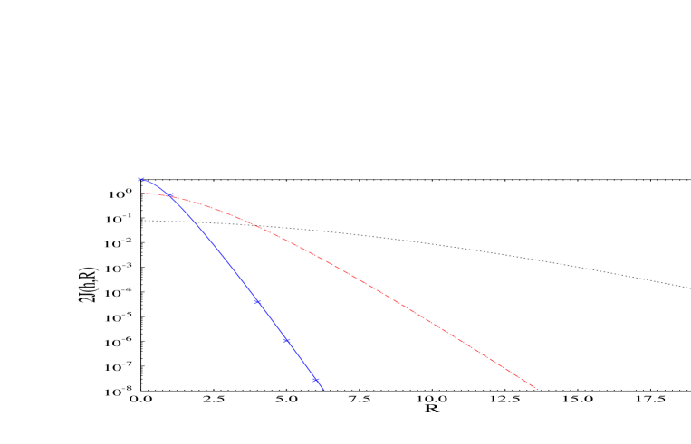
FIG. 4.: The exchange constant as a function of $R$ and $h$. The curves for three different heights are presented. The crosses correspond to the numerical data for $R=0$ and $R=1$ and asymptotic form (11) for the pure two-dimensional case ($h=0$). The solid line is the interpolated formula (56). Dot-dashed and dotted lines present the interpolated formula (54) with $h=0.8$ and 10 respectively.

V Conclusion

We have calculated analytically different limits of the singlet-triplet energy splitting in the two-electron Hamiltonian (1) in the following cases.

1. Hydrogen-like molecule.

   1. $h_{1},h_{2}=0,R>1$, which corresponds to a $2D$ Hydrogen molecule, Eq. (11).

   2. $h_{1,2}\ll 1,\ R>1$, a Hydrogen-like molecule, where perturbation theory is applicable, Eqs. (8,10,14,15).

   3. $1\ll h_{1},h_{2}\ll R$, saddle point method, (Eq. (20)).

2. Helium-like atom.

   1. $R=h_{1}=h_{2}=0$ corresponds to the $2D$ Helium atom, Eq. (26).

   2. $R\ll 1,h_{1}=h_{2}=0$, $2D$ Helium atom with perturbation theory corrections, Eq. (33).

   3. $R=0,h_{1},h_{2}\ll 1$, $2D$ Helium atom with perturbation theory corrections, Eq. (37).

   4. $h_{1},h_{2}>R>1$, quadratic approximation for the Helium-like atom, Eq. (45).

Finally, we have presented the interpolated formula (54) connecting the limits 1 and 2. This formula can be used for calculations of the ground state in spin glasses and semiconductors based on the Heisenberg Hamiltonian. We have shown that the $R$-dependence of the splitting becomes weaker with increasing $h_{1},h_{2}$.

A Eigenvalues and eigenfunctions in $2D$ central potentials

The Schrödinger equation for a radial wave function in a central field is

$$\left\{\frac{\partial^{2}}{\partial r^{2}}+\frac{1}{r}\frac{\partial}{\partial r}-\frac{m^{2}}{r^{2}}-2U(r)+2E\right\}R(r)=0.$$ (A1)

For the Coulomb potential, $U(r)=-Z/r$, the eigenvalues and eigenfunctions are well-known:

$$E_{n} = -\frac{Z^{2}}{2\,(n-1/2)^{2}},$$ (A2)

$$n = 1,2,3...$$ (A3)

$$m = -n+1,-n+2,...n-1$$ (A4)

$$\varphi_{nm}(\vec{r}) = \frac{Ze^{im\phi}}{\sqrt{2\pi}}\sqrt{\frac{16\,(n-|m|-1)!}{(2n-1)^{3}\left[(n+|m|-1)!\right]^{3}}}\left[\frac{4rZ}{2n-1}\right]^{|m|}\exp\left(-\frac{2rZ}{2n-1}\right)L_{n+|m|-1}^{2|m|}\left(\frac{4rZ}{2n-1}\right),$$ (A5)

where $L_{l}^{k}(\rho)$ is the generalized Laguerre polynomials, and the level degeneracy is $g(n)=2n-1$.

The most important for applications here $1s$ and $2s$ states have the following form.

$$\varphi_{10}(r) = \frac{4Z}{\sqrt{2\pi}}e^{-2rZ}$$ (A6)

$$\varphi_{20}(r) = \frac{4Z}{3\sqrt{6\pi}}e^{-2rZ/3}\left[1-\frac{4rZ}{3}\right]$$ (A7)

Thus, for the ground state with $Z=+1$

$$\alpha = 2$$ (A9)

$$A_{\alpha} = \frac{4}{\sqrt{2\pi}}$$ (A10)

Let us consider now the potential

$$U(r)=-1/\sqrt{r^{2}+h^{2}}.$$ (A11)

Far away from the “atomic residue” $U(r)\sim-1/r$ and the wave function for the $s$-state obeys the Schrödinger equation

$$-\frac{\Delta}{2}\varphi-\frac{1}{r}\varphi=-\frac{\alpha^{2}}{2}\varphi$$

with the solution

$$\varphi(r)=A_{\alpha}r^{1/\alpha-1/2}e^{-\alpha r}$$ (A12)

up to $\varphi/r^{2}$ accuracy. Here $A_{\alpha}$ and $\alpha$ are atomic parameters. Their magnitudes are determined by the behavior of the electron inside the “atom”.

The results of the numerical calculations for the normalization constant and the eigenvalues are presented in Figure 5.

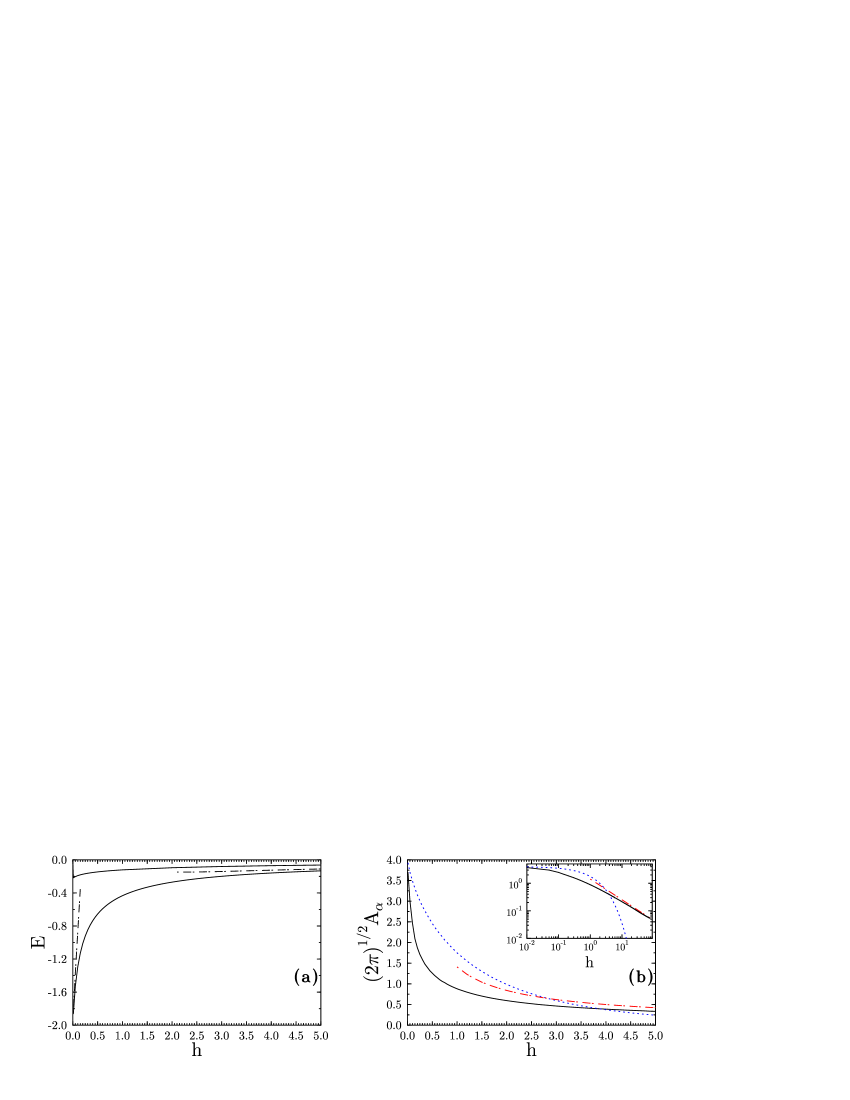
FIG. 5.: (a) Ground and first energies as functions of the parameter $h$. Solid lines are numerical results. The dot-dashed lines correspond to perturbation theory for small $h$ and an asymptotic oscillatory energy $-h^{-1}+h^{-3/2}$ for $h\gg 1$. (b) The constant $A_{\alpha}$ for the ground state. Numerical results (solid line) and analytical estimates for both regimes are shown. Dotted line corresponds to Eq. (A14) and dot-dashed line is the quadratic approximation (A17). The inset is a log-log scale plot.

Simple analytical estimates for the cases of small and large $h$ for ground state energy and the asymptotic coefficient $A_{\alpha}$ can be made.

When $h\ll 1$ the potential is only slightly different from the Coulomb potential and the contribution to the energy can be obtained using perturbation theory:

$$\Delta_{E}=\langle 0|V|0\rangle=16\int_{0}^{\infty}\left(\frac{1}{r}-\frac{1}{\sqrt{h^{2}+r^{2}}}\right)\exp(-4r)r\,dr\approx 16h\left(1+2h\ln(2h)\right)$$ (A13)

Note, that due to the big factor in front of $h$ in (A13) the convergence radius for the perturbation series is small enough.

Supposing that the asymptotic form (A12) of the wave function is valid for all values of $r$, we obtain the following simple estimate for $A_{\alpha}$

$$2\pi A_{\alpha}^{2}\int_{0}^{\infty}r^{2/\alpha}\exp(-2\alpha r)\,dr=1\Rightarrow A_{\alpha}=\frac{2^{1/\alpha-1/2}\alpha^{1/\alpha+1}}{\sqrt{\pi\Gamma(2/\alpha)}}.$$ (A14)

In the opposite case, when $h\gg 1$ the solution has to be close to the oscillatory one

$$E=-\frac{1}{h}+\frac{1}{h^{3/2}}(n+1),$$ (A15)

where $n=0,1,2...$. The main contribution to the normalization comes from the Gaussian part of the wave function because the contribution of the Coulomb tails is negligible. One gets for the state with $n=0$

$$\varphi(r)\approx\varphi_{osc}(r)=\sqrt{\frac{\omega}{\pi}}\exp\left(-\omega r^{2}/2\right),$$ (A16)

where $\omega=1/h^{3/2}$. Then,

$$A_{\alpha}=\frac{1}{\sqrt{\pi}h^{3/4}}.$$ (A17)

The agreement between the behavior of the estimate (A17) and the numerical calculations can be observed in the inset in Fig. 3.

B Exchange constant for $2D$ Hydrogen-like molecule

Since $J(R)$ is exponentially small as $R\rightarrow\infty$, $\Psi_{A}$ and $\Psi_{S}$ are solutions of the same Schrödinger equation, and therefore, with exponential accuracy their combinations

$$\Psi_{1,2}=\frac{\Psi_{S}\pm\Psi_{a}}{\sqrt{2}}$$

are also the solutions of the same Schrödinger equation with the Hamiltonian (1). They correspond to the states of ”distinguishable” particles, when, e.g. for $\Psi_{1}({\bf r_{1},r_{2}})$, the first electron is principally located near first ion at $x=-a$ and the second electron near the second ion with $x=a$. The electron energy

$$E=-\alpha^{2}/2-\beta^{2}/2-1/R,$$

is accurate to terms $\sim 1/R^{2}$. Therefore we are looking for $\Psi_{1,2}$ in a form

$$\Psi_{1}(\vec{r}_{1},\vec{r}_{2}) = \phi_{\alpha}(|\vec{r}_{1}+\vec{a}|)\phi_{\beta}(|\vec{r}_{2}-\vec{a}|)\chi(\vec{r}_{1},\vec{r}_{2}),$$ (B1)

$$\Psi_{2}(\vec{r}_{1},\vec{r}_{2}) = \phi_{\alpha}(|\vec{r}_{2}+\vec{a}|)\phi_{\beta}(|\vec{r}_{1}-\vec{a}|)\chi(\vec{r}_{2},\vec{r}_{1}),$$ (B2)

where $\phi_{\alpha,\beta}$ have an asymptotic behavior (see Appendix A)

$$\varphi_{\alpha}(r)=A_{\alpha}r^{1/\alpha-1/2}e^{-\alpha r},$$

and $\chi$ is a slowly varying function of $\vec{r_{1}},\vec{r_{2}}$. Substituting $\Psi_{1}$ into wave equation and neglecting the second derivatives of $\chi$, we obtain

$$\alpha\frac{\partial\chi}{\partial x_{1}}-\beta\frac{\partial\chi}{\partial x_{2}}+\left[\frac{1}{\sqrt{(x_{1}-x_{2})^{2}+(y_{1}-y_{2})^{2}}}+\frac{1}{2a}-\frac{1}{a-x_{1}}-\frac{1}{a+x_{2}}\right]\chi=0.$$ (B3)

Equation (B3) valid under conditions

$$|x_{1,2}|\leq a,y_{12}\equiv|y_{1}-y_{2}|\ll\sqrt{a}$$ (B4)

$$R\alpha,R\beta\gg 1,R|\alpha-\beta|\ll 1.$$ (B5)

The general solution of (B3) is

$$F(C_{1}(x_{1},x_{2}),C_{2}(\chi,x_{1},x_{2},y_{12})=0,$$ (B6)

where $C_{1},\ C_{2}$ are integrals of the motion of the ordinary differential equations:

$$\frac{dx_{1}}{\alpha}=-\frac{dx_{2}}{\beta}=-\frac{d\chi}{\chi}\left[\frac{1}{\sqrt{(x_{1}-x_{2})^{2}+y_{12}^{2}}}+\frac{1}{2a}-\frac{1}{a-x_{1}}-\frac{1}{a+x_{2}}\right]^{-1}.$$

Hence

$$\frac{dx_{1}}{\alpha}=-\frac{dx_{2}}{\beta}\Rightarrow C_{1}=x_{1}/\alpha+x_{2}/\beta,$$ (B7)

$$\frac{dx_{1}}{\alpha}\left[\frac{1}{\sqrt{(x_{1}-x_{2})^{2}+y_{12}^{2}}}+\frac{1}{2a}-\frac{1}{a-x_{1}}-\frac{1}{a+x_{2}}\right]=-d\ln(\chi)\Rightarrow$$ (B8)

$$C_{2}=\chi\frac{\exp(x_{1}/2a\alpha)[a-x_{1}]^{1/\alpha}[a+x_{2}]^{1/\beta}}{\left[\sqrt{(x_{1}-x_{2})^{2}+y_{12}^{2}}-x_{1}+x_{2}\right]^{\frac{1}{\alpha+\beta}}}$$ (B9)

Combining (B6,B7) we can write the function $\chi$ as

$$\chi(x_{1},x_{2},y_{12})=\frac{\exp\left(-\frac{x_{1}}{2a\alpha}\right)\left[\sqrt{(x_{1}-x_{2})^{2}+y_{12}^{2}}-x_{1}+x_{2}\right]^{\frac{1}{\alpha+\beta}}}{[a-x_{1}]^{1/\alpha}[a+x_{2}]^{1/\beta}}f\left(\frac{x_{1}}{\alpha}+\frac{x_{2}}{\beta}\right),$$ (B10)

where unknown function $f(u)$ is determined from the fact that $\chi\longrightarrow 1$ when $x_{1}\longrightarrow-a,\ x_{2}$ is arbitrary, or when $x_{2}\longrightarrow a$ and $x_{1}$ is arbitrary. Finally, after expanding $|\vec{r}\pm a|\simeq|a\pm x|+y_{12}^{2}/2|a\pm x|$ in the exponent, we obtain

$$\Psi_{1}(\vec{r}_{1},\vec{r}_{2}) = A_{\alpha}A_{\beta}\left(a+x_{1}\right)^{\frac{2-\alpha}{2\alpha}}\left(a-x_{2}\right)^{\frac{2-\beta}{2\beta}}\exp\left[-a(\alpha+\beta)+\beta x_{2}-\alpha x_{1}-\frac{\alpha y_{1}^{2}}{2(a+x_{1})}-\frac{\beta y_{2}^{2}}{2(a-x_{2})}\right]\chi(\vec{r}_{1},\vec{r}_{2}),$$ (B11)

$$\chi(x_{1},x_{2},y_{12}) =$$ (B12)

$$\left\{\begin{array}[]{l}e^{-\frac{a+x_{1}}{2a\alpha}}\left[\frac{2a}{a-x_{1}}\right]^{\frac{1}{\alpha}}\alpha^{-\frac{\alpha}{(\alpha+\beta)\beta}}\left[\frac{\beta(a+x_{1})+\alpha(a+x_{2})}{a+x_{2}}\right]^{\frac{1}{\beta}}\left[\frac{\sqrt{(x_{1}-x_{2})^{2}+y_{12}^{2}}-x_{1}+x_{2}}{\sqrt{\left(\beta(a+x_{1})+\alpha(a+x_{2})\right)^{2}+(\alpha y_{12})^{2}}+\beta(a+x_{1})+\alpha(a+x_{2})}\right]^{\frac{1}{\alpha+\beta}}\\ e^{-\frac{a-x_{2}}{2a\beta}}\left[\frac{2a}{a+x_{2}}\right]^{\frac{1}{\beta}}\beta^{-\frac{\beta}{(\alpha+\beta)\alpha}}\left[\frac{\beta(a-x_{1})+\alpha(a-x_{2})}{a-x_{1}}\right]^{\frac{1}{\alpha}}\left[\frac{\sqrt{(x_{1}-x_{2})^{2}+y_{12}^{2}}-x_{1}+x_{2}}{\sqrt{\left(\beta(a-x_{1})+\alpha(a-x_{2})\right)^{2}+(\beta y_{12})^{2}}+\beta(a-x_{1})+\alpha(a-x_{2})}\right]^{\frac{1}{\alpha+\beta}}\end{array}\right.$$ (B13)

Here the upper expression is given for $x_{1}+x_{2}\leq 0$, and lower expression for $x_{1}+x_{2}\geq 0$ correspondingly.

Substituting (B11) in Eq. (7), and differentiating only the exponent we obtain

$$2J=+2(\alpha+\beta)\int_{-a}^{a}\left[\Psi_{1}\Psi_{2}\right]_{x_{1}=x_{2}=x}\,d\,x\,d\,y_{1}d\,y_{2}$$ (B14)

Introducing notations $\mu=\alpha+\beta$ and $\nu=\beta-\alpha$ and taking into consideration that in the approximation (B4)

$$\sqrt{\left[(\beta+\alpha)(a-x)\right]^{2}+(\beta y_{12})^{2}}+(\beta+\alpha)(a-x)\approx 2(\beta+\alpha)(a-x).$$

the formula (B14) finally transforms to the

$$2J(\alpha,\beta,R)=R^{\frac{2}{\alpha}+\frac{2}{\beta}-\frac{1}{\mu}}e^{-\mu R}\left[D\left(\alpha,\beta,R\right)+D\left(\beta,\alpha,R\right)\right],$$ (B15)

where $D\left(\alpha,\beta,R\right)$ is the following function:

$$D\left(\alpha,\beta,R\right) = 4\sqrt{\pi}A_{\alpha}^{2}A_{\beta}^{2}\left(\frac{\mu}{2}\right)^{-1/\mu}\Gamma\left(\frac{2+\mu}{2\mu}\right)\left(2^{-\mu/\alpha}\frac{\mu}{\alpha}\right)^{\frac{2\alpha}{\mu\beta}}\times$$ (B17)

$$\int_{0}^{1}\frac{\exp\left(-(1-x)/\alpha-\nu Rx\right)(1+x)^{2/\beta-2/\alpha+1/\mu}(1-x)^{2/\alpha-1/\mu}}{\left(1-x\nu/\mu\right)^{1+1/\mu}}dx.$$

In the case $\alpha=\beta$ it is independent of $R$ at all:

$$D_{0}(\alpha)\equiv 2\,D\left(\alpha,\alpha,R\right)=8\sqrt{\pi}A_{\alpha}^{4}\left(\frac{1}{4\alpha}\right)^{1/2\alpha}\Gamma\left(\frac{\alpha+1}{2\alpha}\right)\int_{0}^{1}\exp\left(-t/\alpha\right)(2-t)^{1/2\alpha}t^{3/2\alpha}\,dt.$$ (B18)

In this case

$$2J(\alpha,\alpha,R)=D_{0}(\alpha)R^{7/2\alpha}\exp(-2\alpha R)$$ (B19)

For $2D$ $H_{2}$ molecule ($\alpha=2,\ A_{\alpha}=4/\sqrt{2\pi}$) it gives

$$2J(2,2,R)=30.413\,R^{7/4}\exp(-4R)$$ (B20)

For comparison we remind that in $3D$-case

$$2J_{3D}=1.636R^{5/2}\exp(-2R)$$

REFERENCES

- [1] e-mail: ilya@newt.phys.unsw.edu.au
- [2] S. V. Kravchenko et al., Phys. Rev. Lett., 77, 4938 (1996).
- [3] D. Simonian et al., Phys. Rev. Lett., 79, 2304 (1997).
- [4] I. V. Ponomarev, V. V. Flambaum, A. L. Efros, Phys. Rev. B, (1999) to be published.
- [5] L. P. Gorkov and L. P. Pitaevskii, Soviet Phys. Doklady, 8, 788 (1964); C.Herring and M. Flicker, Phys. Rev., 134, A362 (1964).
- [6] B. M. Smirnov and M. I. Chibisov, Soviet Phys. JETP, 21, 624 (1965).
- [7] V. V. Flambaum, I. V. Ponomarev, and O. P. Sushkov, Phys Rev. B, 59, 4163 (1999).
- [8] G. Staszewska and L. Wolniewicz, J. Mol. Specroscopy, 1999 (to be published); W. Kolos and L. Wolniewicz, Chem. Phys. Lett., 24, 457 (1974); L. Wolniewicz, JCP 99, 1851 (1993)
- [9] We found that for three-dimensional hydrogen molecule and .