Quantum Phase Transitions in Two-Dimensional Spin Systems with Ladder, Plaquette and Mixed-Spin Structures

1 Introduction

Recently low-dimensional spin systems with the gap for the excitation spectrum have been the subjects of considerable interest. The spin gap is generated by various mechanisms, which may be sensitive to the lattice structure, the competing interactions, the topological nature of spins, etc. A typical example is the spin plaquette system such as $\rm CaV_{4}O_{9}$, ${}^{\hbox{\immediate{\bf{?}},\penalty 1000\hskip 0.91003pt plus 0.70004pt minus 0.70004pt{\bf{?}},\penalty 1000\hskip 0.91003pt plus 0.70004pt minus 0.70004pt{\bf{?}},\penalty 1000\hskip 0.91003pt plus 0.70004pt minus 0.70004pt{\bf{?}},\penalty 1000\hskip 0.91003pt plus 0.70004pt minus 0.70004pt{\bf{?}},\penalty 1000\hskip 0.91003pt plus 0.70004pt minus 0.70004pt{\bf{?}},\penalty 1000\hskip 0.91003pt plus 0.70004pt minus 0.70004pt{\bf{?}},\penalty 1000\hskip 0.91003pt plus 0.70004pt minus 0.70004pt{\bf{?}})}}$ which may be described by the two-dimensional (2D) Heisenberg model on a 1/5 depleted square lattice or the meta-plaquette model.${}^{\hbox{\immediate{?},\penalty 1000\hskip 0.91003pt plus 0.70004pt minus 0.70004pt{?})}}$ The disordered ground state with the spin gap observed in these systems may result from the singlet-spin configuration formed in each plaquette. Another prototypical example is the coupled spin-ladder system${}^{\hbox{\immediate{\bf{?}})}}$ realized in the compounds such as SrCu₂O₃${}^{\hbox{\immediate{\bf{?}},\penalty 1000\hskip 0.91003pt plus 0.70004pt minus 0.70004pt{\bf{?}})}}$ and (Sr, Ca)₁₄Cu₂₄O₄₁.${}^{\hbox{\immediate{\bf{?}})}}$ For such ladder systems with even number of legs, the spin gap is generated to stabilize the disordered ground state. Interestingly enough, the introduction of non-magnetic impurities into this system induces the phase transition to the magnetically ordered state.${}^{\hbox{\immediate{?},\penalty 1000\hskip 0.91003pt plus 0.70004pt minus 0.70004pt{?},\penalty 1000\hskip 0.91003pt plus 0.70004pt minus 0.70004pt{\bf{?}})}}$ Furthermore, to the family of the spin gap systems we may add the mixed-spin system, in which the topological nature of spins as well as the lattice structure play an essential role to produce the spin gap. For instance, in one-dimensional (1D) systems, a mixed-spin chain with the alternating array of two kinds of spins has stimulated intensive experimental${}^{\hbox{\immediate{\bf{?}})}}$ and theoretical${}^{\hbox{\immediate{\bf{?}},\penalty 1000\hskip 0.91003pt plus 0.70004pt minus 0.70004pt{\bf{?}},\penalty 1000\hskip 0.91003pt plus 0.70004pt minus 0.70004pt{\bf{?}},\penalty 1000\hskip 0.91003pt plus 0.70004pt minus 0.70004pt{\bf{?}},\penalty 1000\hskip 0.91003pt plus 0.70004pt minus 0.70004pt{\bf{?}})}}$ studies. It is known that the 1D mixed-spin chain realizes either the ferrimagnetic or the singlet ground state depending on how we arrange different type of spins on the 1D lattice.${}^{\hbox{\immediate{?},\penalty 1000\hskip 0.91003pt plus 0.70004pt minus 0.70004pt{?},\penalty 1000\hskip 0.91003pt plus 0.70004pt minus 0.70004pt{?})}}$

Various spin gap systems mentioned above provide us with an interesting research area of quantum spin systems. Among others, the quantum phase transition from the spin gap phase to the magnetically ordered phase is one of the most interesting issues. Motivated by these hot topics we investigated in the previous paper${}^{\hbox{\immediate{\bf{?}})}}$ the competition between the magnetically ordered and disordered states in the 2D quantum spin system which includes both of the bond- and spin-alternations. By means of the non-linear sigma model and the modified spin wave approach, we evaluated the spin gap and the spontaneous staggered magnetization to discuss the quantum phase transitions. Although this study enabled us to qualitatively describe how the spin gap phase is driven to the antiferromagnetic one, the resulting phase diagram was not sufficient enough to give quantitative discussions.

The purpose of the present work is to study more quantitatively the quantum phase transitions for the 2D spin systems with ladder, plaquette, and mixed-spin structures. To this end we employ the series expansion method developed${}^{\hbox{\immediate{\bf{?}},\penalty 1000\hskip 0.91003pt plus 0.70004pt minus 0.70004pt{\bf{?}})}}$ and extensively used by many groups for ladders,${}^{\hbox{\immediate{\bf{?}})}}$ 2D systems,${}^{\hbox{\immediate{?},\penalty 1000\hskip 0.91003pt plus 0.70004pt minus 0.70004pt{\bf{?}},\penalty 1000\hskip 0.91003pt plus 0.70004pt minus 0.70004pt{\bf{?}})}}$ Kondo lattice models,${}^{\hbox{\immediate{\bf{?}})}}$ bilayer systems,${}^{\hbox{\immediate{\bf{?}})}}$ etc. In this approach, starting with properly chosen singlet-spin clusters, we introduce the couplings among the clusters perturbatively to carry out the series expansion of the physical quantities such as the staggered susceptibility. Then the critical point for the phase transition is determined by applying the Padé approximants${}^{\hbox{\immediate{\bf{?}})}}$ to the physical quantities thus obtained.

The paper is organized as follows. In §2, we first introduce the Hamiltonian for 2D spin systems and outline how to apply the series expansion techniques to our systems. In §3, by performing the series expansion for the staggered susceptibility and then employing the Padé approximants, we obtain the phase diagram to discuss the competition between the disordered and ordered states for three kinds of 2D quantum spin systems mentioned above. Brief summary is given in the last section.

2 Cluster Expansions

We consider a 2D antiferromagnetic quantum spin system, which is described by the following generalized Heisenberg Hamiltonian

$$H = H_{0}+H_{1},$$ (2.1)

$$H_{0} = J_{1}\sum_{(i,j)\in D_{1}}\mbox{\boldmath$S$}_{i}\cdot\mbox{\boldmath$S$}_{j},$$ (2.2)

$$H_{1} = J_{2}\sum_{(i,j)\in D_{2}}\mbox{\boldmath$S$}_{i}\cdot\mbox{\boldmath$S$}_{j}+J_{3}\sum_{(i,j)\in D_{3}}\mbox{\boldmath$S$}_{i}\cdot\mbox{\boldmath$S$}_{j},$$ (2.3)

where $\mbox{\boldmath$S$}_{j}$ is the spin operator at the $j$-th site on the square lattice and $J_{1}$, $J_{2}$, and $J_{3}$ are the antiferromagnetic exchange couplings ($J_{1},J_{2},J_{3}>0$). Note that the spin $\mbox{\boldmath$S$}_{j}$ is allowed to take different values at each cite, which enables us to treat the systems with mixed spins.

In order to apply cluster expansion techniques,${}^{\hbox{\immediate{?})}}$ the Hamiltonian is divided into two parts. Since we start with a strong-coupling singlet state, we take the unperturbed Hamiltonian $H_{0}$ as an assembly of independent singlet-spin clusters formed by the coupling $J_{1}$ (the corresponding bonds $(i,j)$ are sepecified by $D_{1}$). The interactions among independent clusters are then taken into account by series expansions in the perturbed term $H_{1}$. We introduce two types of perturbations, for which the corresponding sets of bonds $(i,j)$ are denoted by $D_{2}$ and $D_{3}$. The detail of $D_{1},D_{2}$, and $D_{3}$ will be given for each case in the following sections. We henceforth assume that $\lambda(\equiv J_{2}/J_{1})<1$ and $\alpha\lambda(\equiv J_{3}/J_{1})<1(0<\alpha<1)$. We will see that this parameter regime indeed includes physically interesting cases.

In the following, we discuss the quantum phase transitions for the 2D antiferromagnetic spin systems with ladder, plaquette, and mixed-spin structures. To this end, we introduce three kinds of singlet-cluster configurations, i.e., the dimer singlet, the plaquette singlet, and the mixed-spin-cluster singlet. The last one, which is unique for our systems, is composed of a specific singlet-spin configuration, e.g. $1/2\circ 1\circ 1/2$ (see Figs. 8 and 9). The introduction of the mixed-spin-cluster allows us to perform a systematic series expansion for 2D mixed spin systems. Starting with the above spin singlet states, we can carry out the series expansion with respect to $\lambda$ as well as $\alpha\lambda$. For the ladder, the plaquette, and the mixed-spin structures, we refer to the corresponding expansions as the dimer, the plaquette, and the mixed spin-cluster expansions, respectively. We naturally expect that the introduction of $H_{1}$ perturbs the singlet ground state with the excitation gap and gradually enhances the antiferromagnetic spin correlations, finally giving rise to the long-range magnetic order. This will be shown to be indeed the case for our systems.

We calculate the staggered spin susceptibility to determine the critical point for the transition. We thus add the following Zeeman term as a perturbation,

$$H_{\rm ST}=h\left[\sum_{i\in A}S_{i}^{z}-\sum_{i\in B}S_{i}^{z}\right],$$ (2.4)

where $h$ is the staggered magnetic field and $A$ ($B$) denotes one of the two sublattices. We estimate the ground state energy $E(h)$ of the total Hamiltonian $H+H_{\rm ST}$ up to the second order in $h$, and then obtain the magnetic susceptibility $\chi$ for the staggered field,

$$\chi=-\left.\frac{\partial^{2}E(h)}{\partial h^{2}}\right|_{h=0}.$$ (2.5)

This quantity is expanded as a power series in $\lambda$ as

$$\chi=\sum_{n=0}a_{n}\lambda^{n}.$$ (2.6)

We calculate the susceptibility up to the eighth order in $\lambda$ for the dimer expansion and the fourth order for both of the plaquette and the mixed-spin cluster expansions. We should recall here that the phase boundary between the magnetically ordered and disordered states is given by the critical line on which the staggered susceptibility is divergent. Therefore a further approximate procedure is necessary to deduce the sensible singularity by the asymptotic analysis of the power-series expansion. For this purpose, we make use of Padé approximants${}^{\hbox{\immediate{?})}}$ for the susceptibility obtained up to the finite order in $\lambda$. Besides ordinary Dlog Padé approximants, we also employ biased Padé approximants,${}^{\hbox{\immediate{?})}}$ for which we assume that the phase transition in our 2D quantum spin models should belong to the universality class of the 3D classical Heisenberg model.${}^{\hbox{\immediate{\bf{?}})}}$ Then the critical value of $\lambda_{c}$ is determined by the formula $\chi\sim(\lambda-\lambda_{c})^{-\gamma}$ with the known exponent $\gamma=1.4$.${}^{\hbox{\immediate{\bf{?}})}}$ We shall see below that the biased method provides a fairly good approximation for $\lambda_{c}$ in some cases, and in general is useful to check how well our Padé approximants work.

3 Quantum Phase Transitions

In this section, we discuss the quantum phase transitions by applying the series expansion to our models. We have two parameters in the perturbed term, $\lambda$ and $\alpha$, so that we can observe in different ways how the 2D antiferromagnetic correlations develop. To confirm the validity of our series expansions and Padé approximants, we first study the 2D system with ladder structure which was already studied extensively by various methods. Our results are compared with those of the quantum Monte Carlo (QMC) simulation in rather good agreement.${}^{\hbox{\immediate{\bf{?}},\penalty 1000\hskip 0.91003pt plus 0.70004pt minus 0.70004pt{\bf{?}},\penalty 1000\hskip 0.91003pt plus 0.70004pt minus 0.70004pt{\bf{?}})}}$ We then move to the plaquette spin systems and the mixed spin systems, and argue how the plaquette-singlet state and the mixed-spin singlet state are driven to the 2D magnetically ordered state.

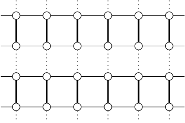
Fig.  1: 2D spin system with the ladder structure. The circle represents the spin $s=1/2$. We refer to the system as the coupled-ladder (coupled-dimer-chain) system, when the bold, the thin, and the dashed lines represent the coupling constants $1$, $\lambda_{\rm L}(\alpha_{\rm D}\lambda_{\rm D})$, and $\alpha_{\rm L}\lambda_{\rm L}(\lambda_{\rm D})$, respectively.

3.1 Ladder-structure systems

Let us start with a 2D spin system with the ladder structure, which is shown schematically in Fig. 1. In this figure, the circle represents the $s=1/2$ spin sitting on the square lattice. Note that this 2D model can be constructed from isolated dimers in two ways depending on how we may introduce the couplings among dimers perturbatively: we may refer to the system correspondingly as the coupled 2-leg ladders and the coupled dimer chains. In the former case, the bold, the thin, and the dashed lines in Fig. 1 represent the coupling constants $1(=J_{1}),\lambda_{\rm L}(=J_{2})$, and $\alpha_{\rm L}\lambda_{\rm L}(=J_{3})$, respectively. By tuning the value of $\alpha_{\rm L}$, we naturally interpolate the independent 2-leg ladders ($\alpha_{\rm L}=0$) and the 2D systems. On the other hand, in the latter case, by taking $1(=J_{1}),\lambda_{\rm D}(=J_{3})$, and $\alpha_{\rm D}\lambda_{\rm D}(=J_{2})$, we can investigate how the independent dimer chains ($\alpha_{\rm D}=0$) are combined to make the 2D systems. We distinguish these two constructions which may be complementary to each other because the available parameter regime is restricted in our series expansion approach.

Fig.  2: Phase diagram for the coupled-ladder system in Fig. 1. The solid (dashed) line indicates the phase boundary obtained by the biased [3/4] (Dlog [3/4]) Padé approximants. The filled circles represent the results of the QMC simulations. ${}^{\hbox{\immediate{?},\penalty 1000\hskip 0.91003pt plus 0.70004pt minus 0.70004pt{?},\penalty 1000\hskip 0.91003pt plus 0.70004pt minus 0.70004pt{?})}}$

Let us first regard the 2D system as the coupled 2-leg ladders as shown in Fig. 1. The starting Hamiltonian $H_{0}$ has the ground state with the spin gap due to the dimer singlets. We calculate the staggered susceptibility $\chi$ by means of the dimer expansion up to eighth order in $\lambda_{\rm L}$ for various values of $\alpha_{\rm L}$. The resulting power series for some particular values of $\alpha_{\rm L}$ are presented in Table I.

Table  I: Series coefficients $a_{n}$ for the dimer expansion of the staggered susceptibility per site $\chi$ for the coupled-ladder system.

n	$\alpha_{\rm L}=0.0$	$\alpha_{\rm L}=0.2$	$\alpha_{\rm L}=0.5$	$\alpha_{\rm L}=1.0$
0	1.0000000	1.0000000	1.0000000	1.0000000
1	2.0000000	2.2000000	2.5000000	3.0000000
2	2.5000000	3.3350000	4.7187500	7.3750000
3	1.7500000	3.7765000	7.7265625	17.062500
4	-0.44791667	2.9802427	11.400106	37.401693
5	-2.7586806	1.3427618	16.016045	79.689670
6	-2.6446759	0.32560333	22.218817	165.96349
7	1.2087764	1.3087535	30.989600	340.66295
8	5.9745629	3.6797174	43.252600	692.38191

Using Padé approximants, we get the phase diagram shown in Fig. 2. In this figure, the solid (dashed) line represents the phase boundary obtained by the biased [3/4] (Dlog [3/4]) Padé approximants. When $\alpha_{\rm L}=0$, the system is reduced to the isolated 2-leg ladders with the interleg (intraleg) coupling constant $1$ ($\lambda_{\rm L}$), which is known to have disordered ground state with spin gap.${}^{\hbox{\immediate{?})}}$ Increasing the parameter $\alpha_{\rm L}$ with a fixed $\lambda_{\rm L}$, the antiferromagnetic correlation grows up, and eventually the phase transition to the antiferromagnetically ordered state occurs. For instance, if we determine the phase boundary by means of biased [3/4] Padé appoximants, the critical value is given by $\alpha_{\rm L}=0.26$ for $\lambda_{\rm L}=1$.

We find that near $\alpha_{\rm L}\sim 0.8$ the phase boundary determined by the Dlog Padé approximants exhibits a pathological behavior, namely it branches out into upper and lower lines. It may be obvious that these lines may not be physically sensible. It is known that this type of pathology occasionally appears in Padé approximants. If we discard these spurious parts in critical lines, we then find that the results of two Padé approximants show the common behavior and are both in good agreement with those of the QMC simulations.${}^{\hbox{\immediate{?},\penalty 1000\hskip 0.91003pt plus 0.70004pt minus 0.70004pt{?},\penalty 1000\hskip 0.91003pt plus 0.70004pt minus 0.70004pt{?})}}$ Also, our results reproduce the critical value $\lambda_{\rm L}=0.54$ for $\alpha_{\rm L}=1$ which was previously obtained by Singh et al. ${}^{\hbox{\immediate{?})}}$ We should notice, however, that the biased Padé approximants may not always give more accurate results than the ordinary Dlog Padé approximants. We must carefully determine the phase boundary after trying various Padé approximants, as will be momentarily shown below.

Fig.  3: Phase diagram for the coupled-dimer-chain system in Fig. 1. The solid (dotted) line indicates the phase boundary obtained by the Dlog [4/3] (biased [4/3]) Padé approximants. The filled circles represent the QMC simulation results. ${}^{\hbox{\immediate{?},\penalty 1000\hskip 0.91003pt plus 0.70004pt minus 0.70004pt{?})}}$

We next regard the present system as the coupled dimer chains, for which the corresponding couplings are defined in Fig. 1. Repeating a similar calculation as in the previous case, we arrive at the phase diagram shown in Fig. 3. We list the obtained series for some values of $\alpha$ in Table II.

Table  II: Series coefficients $a_{n}$ for the dimer expansion of the staggered susceptibility per site $\chi$ for the coupled-dimer-chain system.

n	$\alpha_{\rm D}=0.0$	$\alpha_{\rm D}=0.2$	$\alpha_{\rm D}=0.5$	$\alpha_{\rm D}=1.0$
0	1.0000000	1.0000000	1.0000000	1.0000000
1	1.0000000	1.4000000	2.0000000	3.0000000
2	0.87500000	1.7750000	3.5000000	7.3750000
3	0.81250000	2.2865000	6.0312500	17.062500
4	0.77669271	2.9068927	10.016927	37.401693
5	0.74435764	3.6732624	16.341092	79.689670
6	0.71753608	4.6106279	26.245183	165.96349
7	0.69609122	5.7558135	41.690073	340.66295
8	0.67767823	7.1518929	65.617441	692.38191

In this figure, the solid and the dotted lines represent the phase boundaries obtained by the Dlog [4/3] and the biased [4/3] Padé approximants. In the latter analysis, we have two critical lines, one of which (labeled by crosses) exhibits a pathological behavior quite different from that of the Dlog Padé analysis. If we discard this line, we find that the results of two Padé approximants show the physically sensible behavior and are consistent with those of the QMC simulations${}^{\hbox{\immediate{?},\penalty 1000\hskip 0.91003pt plus 0.70004pt minus 0.70004pt{?})}}$ (the filled circles in Fig. 3).

Finally we wish to note that at the point $(\alpha_{\rm D},\lambda_{\rm D})=(0,1)$, our system just lies on the critical line which separates the ordered and disordered states, as seen from Fig. 3. Since the system in this case is reduced to the independent isotropic spin chains, our numerical results reproduce the well-known fact that the ground state of the spin-1/2 Heisenberg chain is in a critical spin liquid phase, so-called Tomonaga-Luttinger liquid phase, with neither the spin gap nor the long-range order.${}^{\hbox{\immediate{\bf{?}})}}$ We also note that the properties around this quantum critical point have been already studied by Affleck et al.${}^{\hbox{\immediate{?})}}$

The above studies on the ladder-structure systems seem to give rather satisfactory results, which encourage us to apply a similar series expansion approach to the analysis of other quantum spin systems.

3.2 Plaquette-structure systems

Let us now turn to the plaquette spin systems. We here consider two kinds of the models. First, we are concerned with the system shown in Fig. 4. The starting Hamiltonian $H_{0}$ describes a sum of the independent plaquettes, whose ground state is spin singlet with the excitation gap. Introducing the perturbed part $H_{1}$ may induce the competition between the plaquette-singlet correlation and the antiferromagnetic one. By this construction of the system, we naturally interpolate the isolated plaquettes $\lambda=0$ (or isolated ladders $\alpha=0$) and the normal square lattice.

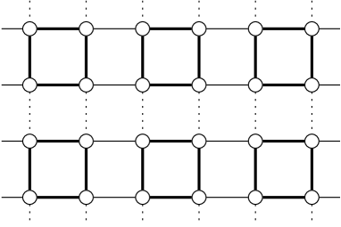
Fig.  4: 2D spin system with the plaquette structure. The circle represents the spin $s=1/2$. The bold, the thin, and the dashed lines represent the coupling constants 1, $\lambda$, and $\alpha\lambda$.

Fig.  5: Phase diagram for the plaquette system in Fig. 4. The solid line indicates the phase boundary obtained by the biased [1/2] Padé approximants.

The coefficients are calculated up to the fourth order in $\lambda$ by means of the plaquette expansion and tabulated in Table III for some particular values of $\alpha$.

Table  III: Series coefficients $a_{n}$ for the plaquette expansion of the staggered susceptibility per site $\chi$ for the 2D spin system with the plaquette structure.

n	$\alpha=0.0$	$\alpha=0.2$	$\alpha=0.5$	$\alpha=1.0$
0	1.3333333	1.3333333	1.3333333	1.3333333
1	1.7777778	2.1333333	2.6666667	3.5555556
2	1.6009195	2.6131044	4.3715197	7.9425797
3	1.1215579	2.9136374	6.8339620	17.102341
4	0.5614964	3.0347609	10.187867	35.146612

Using the biased [1/2] Padé approximants, we obtain the phase diagram shown in Fig. 5. In this phase diagram the system on the $\alpha=0$ axis is composed of the assembly of the independent 2-leg ladders, which belongs to the disordered spin-gap phase. Away from this axis, the 2D antiferromagnetic correlation grows up and the quantum phase transition to the ordered state occurs at the critical value $\alpha_{c}$. When $\lambda=1$, we find $\alpha_{c}=0.22$. We note that this plaquette system with $\lambda=1$ is equivalent to the coupled 2-leg ladders with $\lambda_{\rm L}=1$ discussed in the previous subsection, where we have obtained the slightly different critical value $\alpha_{\rm L}=0.26$. It is also to be noticed that the mean-field theory by the bond-operator representation and the QMC simulation also yield the corresponding values $\alpha_{c}=0.25$${}^{\hbox{\immediate{\bf{?}})}}$ and $0.32$${}^{\hbox{\immediate{?})}}$ for the system with $\lambda=1$. These results imply that it may be necessary to carry out higher order cluster expansions both for dimer and plaquette systems to obtain more accurate critical values of $\alpha$ in the region $\lambda$ $\stackrel{{\scriptstyle\scriptstyle>}}{{\scriptstyle\sim}}$ $1$ (This is indeed seen from Fig. 2 for the ladder system). Finally we wish to mention that for the special case ($\alpha=1$), where each plaquette is connected with nearest neighbor ones via the single coupling constant $\lambda$, similar results have been reported by Fukumoto and Oguchi.${}^{\hbox{\immediate{\bf{?}})}}$

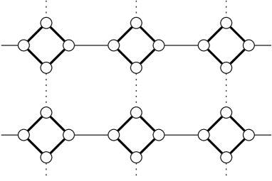
Fig.  6: 2D spin system composed of the plaquette chains. The circle represents the spin $s=1/2$. The bold, the thin, and the dashed lines indicate the coupling constants 1, $\lambda$, and $\alpha\lambda$.

Fig.  7: Phase diagram for the plaquette system in Fig. 6. The solid line represents the phase boundary obtained by the biased [2/2] Padé approximants.

Let us next consider the system shown in Fig. 6, which may be considered to be made out of plaquette chains,${}^{\hbox{\immediate{?},\penalty 1000\hskip 0.91003pt plus 0.70004pt minus 0.70004pt{\bf{?}},\penalty 1000\hskip 0.91003pt plus 0.70004pt minus 0.70004pt{?})}}$ because this model, for $\alpha=0$ with finite $\lambda$, is reduced to the isolated chains with plaquette structures. An interesting point is that this system is topologically equivalent to the 1/5 depleted square lattice ${}^{\hbox{\immediate{?},\penalty 1000\hskip 0.91003pt plus 0.70004pt minus 0.70004pt{?},\penalty 1000\hskip 0.91003pt plus 0.70004pt minus 0.70004pt{?})}}$ which is relevant to the study for the compound ${\rm CaV_{4}O_{9}}$. The phase diagram shown in Fig. 7 is obtained by the fourth order calculation and the biased [2/2] Padé approximants. The resulting series for some values of $\alpha$ are listed in Table IV.

Table  IV: Series coefficients $a_{n}$ for the plaquette expansion of the staggered susceptibility per site $\chi$ for the 2D spin system composed of the plaquette chains.

n	$\alpha=0.0$	$\alpha=0.2$	$\alpha=0.5$	$\alpha=1.0$
0	1.3333333	1.3333333	1.3333333	1.3333333
1	0.88888889	1.0666667	1.3333333	1.7777778
2	0.47985790	0.73608925	1.1924150	2.1449010
3	0.20889382	0.47565756	1.0634199	2.6268926
4	0.073161406	0.29653125	0.92711496	3.1394401

Let us first look at the results with the value of $\lambda$ being fixed. By increasing the value of $\alpha$ from zero, we observe the evolution of the plaquette chain to the depleted square lattice. For example, in the case of $\lambda=1$, we get the critical value $\alpha_{c}=0.82$. On the other hand, when we fix $\alpha=1$, we can see how the isolated plaquettes are uniformly coupled to form the 1/5 depleted square lattice, for which we obtain the critical value $\lambda_{c}=0.91$. This value is in good agreement with the result already obtained by QMC ${}^{\hbox{\immediate{?})}}$ and also by the plaquette expansion.${}^{\hbox{\immediate{?})}}$ As clear from these results, the plaquette structure is quite essential, but is not sufficient to produce the spin gap for the isotropic 1/5 depleted square lattice ($\lambda=\alpha=1$), for which we have the antiferromagnetic long-range order. So, it is necessary to introduce the dimer structure or frustrating couplings to have the spin gap in this case.${}^{\hbox{\immediate{?},\penalty 1000\hskip 0.91003pt plus 0.70004pt minus 0.70004pt{?})}}$

3.3 Mixed-spin systems

So far, we have restricted our discussions to the 2D spin-1/2 systems, for which the lattice structure plays an important role to generate the spin gap. As mentioned in the introduction, the mixed-spin systems with periodic array of different spins also have attracted much attention both experimentally and theoretically. In these systems, not only the lattice structure but also the topological nature of spins become important for the gap formation. In the previous papers,${}^{\hbox{\immediate{?},\penalty 1000\hskip 0.91003pt plus 0.70004pt minus 0.70004pt{?})}}$ we have investigated how the 1D mixed spin chains are coupled to form the 2D mixed spin system by means of the non-linear $\sigma$ model and the modified spin wave analysis. Although the quantum phase transitions between magnetically ordered and disordered phases were described at least qualitatively by the above approaches, the results obtained turned out to be far from quantitative discussions. The purpose in this subsection is to quantitatively explore the phase transitions in 2D mixed spin systems by using the series expansion method. To be specific, we wish to deal with two typical systems composed of $s=1/2$ and $s=1$, which are shown in Figs. 8 and 9.

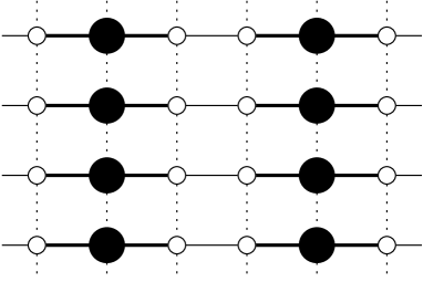
Fig.  8: 2D spin system with the columnar mixed-spin structure. The small (large filled) circle represents $s=1/2$ ($s=1$). The bold, the thin, and the dashed lines indicate the coupling constants $1$, $\lambda$, and $\alpha\lambda$.

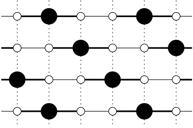
Fig.  9: 2D spin system with the diagonal mixed-spin structure. The small (large filled) circle represents $s=1/2$ ($s=1$). The bold, the thin, and the dashed lines indicate the coupling constants $1$, $\lambda$, and $\alpha\lambda$.

Let us first consider the system shown in Fig. 8, which we refer to as the ”columnar mixed-spin system”, for which the mixed spin chains are stacked uniformly in a vertical direction. In this figure, the small circle (large filled circle) represents $s=1/2(s=1)$ and the bold, the thin, and the dashed lines indicate the coupling constants $1(=J_{1}),\lambda(=J_{2})$, and $\alpha\lambda(=J_{3})$, respectively. When $\lambda=0(H_{1}=0)$, the wave function of the ground state is the direct product of mixed-spin-cluster singlets given by the spin arrangement of $1/2\circ 1\circ 1/2$. This is our starting configuration for the cluster expansion. The phase transition to the ordered state may be anticipated when the values of $\alpha$ and $\lambda$ are increased. We perform the mixed-spin cluster expansion up to the fourth order and list the series coefficients for some particular values of $\alpha$ in Table V.

Table  V: Series coefficients $a_{n}$ for the mixed-spin cluster expansion of the staggered susceptibility per site $\chi$ for the columnar mixed-spin system.

n	$\alpha=0.0$	$\alpha=0.2$	$\alpha=0.5$	$\alpha=1.0$
0	1.7777778	1.7777778	1.7777778	1.7777778
1	1.1851852	2.6074074	4.7407407	8.2962963
2	0.63981053	3.2769402	10.010760	28.642125
3	0.27852509	4.0253708	20.019578	88.590346
4	0.097548541	4.7431208	38.497553	259.24615

Employing the biased [2/1] Padé approximants for the staggered susceptibility, we end up with the phase diagram shown in Fig. 10 (solid line). We find that the system at the point $(\alpha,\lambda)=(0,1)$, which consists of independent mixed-spin chains, is in a disordered phase with spin gap. This result correctly reproduces the fact that the low-energy excitation in the present mixed spin chain has a gap, which is deduced via the topological properties of the system.${}^{\hbox{\immediate{?},\penalty 1000\hskip 0.91003pt plus 0.70004pt minus 0.70004pt{?})}}$ We note that for $\lambda=1$ the phase transition to the ordered phase occurs at the critical value $\alpha_{c}=0.16$.

Fig.  10: The phase diagram for the systems in Fig. 8 (the solid line) and Fig. 9 (the dashed line). The critical lines are determined by the biased [2/1] Padé approximants.

Next we turn to the system shown in Fig. 9. We refer to it as the ”diagonal mixed-spin system” since the mixed spin chains ($\alpha=0$) are stacked diagonally. The definition of the coupling constants is the same as that in Fig. 8. The mixed-spin cluster expansion up to the fourth order with the biased [2/1] Padé approximants yields the phase diagram shown in Fig. 10 (the dashed line). We tabulates the resulting series for some values of $\alpha$ in Table VI.

Table  VI: Series coefficients $a_{n}$ for the mixed-spin cluster expansion of the staggered susceptibility per site $\chi$ for the diagonal mixed-spin system.

n	$\alpha=0.0$	$\alpha=0.2$	$\alpha=0.5$	$\alpha=1.0$
0	1.7777778	1.7777778	1.7777778	1.7777778
1	1.1851852	2.3703704	4.1481481	7.1111111
2	0.63981053	2.8229887	8.3587481	23.614326
3	0.27852509	3.1554307	15.787595	73.062503
4	0.097548541	3.3658619	28.541914	216.50885

For $\alpha=0$, the system is correctly reduced to an assembly of isolated mixed-spin chains which have the disordered ground state. For $\lambda=1$ the phase transition to the ordered phase occurs at the critical value $\alpha_{c}=0.21$.

Carefully observing Fig. 10 one notices that two critical lines intersect each other in the vicinity of $\alpha=0.87$. In the region $\alpha<0.87$, the area of the disordered phase for the diagonal system is larger than that for the columnar one. This implies that when we increase $\lambda$ or $\alpha$ in this region, the antiferromagnetic correlation among spin clusters grows up more easily in the columnar system than in the diagonal one, because larger spins ($s=1$) are directly coupled with each other in the columnar case, and stabilize the long-range order more effectively.

On the other hand, when $\alpha>0.87$, the situation is reversed, namely, the disordered phase in the columnar system is more stable than that for the diagonal system. This may be understood by observing the behavior in the limit $\alpha\rightarrow\infty$. In this limit, the columnar system is reduced to the three-leg ladder, ${}^{\hbox{\immediate{?})}}$ while the diagonal one still forms the 2D network. Recall here that this three-leg ladder consists of two $s=1/2$ chains and one $s=1$ chain, which is known to have the spin gap.${}^{\hbox{\immediate{?},\penalty 1000\hskip 0.91003pt plus 0.70004pt minus 0.70004pt{?})}}$ Therefore, in the limit of $\alpha\rightarrow\infty$ the 2D antiferromagnetic correlation vanishes for the columnar system, while it may still survive for the diagonal one. This may explain the behavior observed in the region $\alpha>0.87$.

Up to now, the mixed-spin chains found experimentally are known to exhibit the ferrimagnetic ground state.${}^{\hbox{\immediate{?})}}$ It may be expected that the mixed-spin chains with singlet ground state, as discussed here, may be also synthesized experimentally in the future. It would thus be an interesting subject to observe how such disordered systems are driven to the magnetically ordered phase in the presence of the interchain couplings, impurities, etc.

4 Summary

We have investigated the quantum phase transitions in the 2D spin systems with ladder, plaquette, and mixed-spin structures. In order to quantitatively study the phase transitions, we have employed the systematic cluster expansion methods. It has turned out that the present approach improves to large extent our previous results on the phase diagram obtained by the non-linear $\sigma$ model as well as the modified spin wave analysis. For example, from the results on the ladder-structure systems we have confirmed that the dimer expansion analysis is comparable to the QMC simulation in some parameter regions. We have also studied the phase diagrams for the spin systems with the plaquette and the mixed-spin structures. For plaquette systems, starting with isolated plaquettes we have introduced the couplings among the plaquettes in two distinct ways: the one is naturally extrapolated to the 2D square lattice, while the other is to the 1/5 depleted square lattice. In particular, for the latter case, we have clarified how the plaquette chains studied previously are coupled to form the 1/5 depleted square lattice system. Also, for the mixed spin systems, we have considered two ways for stacking the spin chains, which are referred to as the columnar and diagonal systems. It has been pointed out that the stability of the disordered phase non-trivially depends on how to stack the mixed spin chains.

In this paper we have concentrated on the staggered susceptibility to establish the phase diagram. Not only to confirm our present results but also to get further information, it is desirable to calculate the elementary excitation spectrum in the same framework of the cluster expansion. In this direction, we have performed a preliminary calculation of the spin excitation gap for the columnar mixed spin system up to the fifth order in the coupling constant. The phase boundary determined in this way turns out to be in fairly good agreement with the one shown in Fig. 10. We thus believe that the present analysis of the staggered susceptibility, although it has been restricted to the fourth order, already captures essential properties of the spin systems discussed in this paper.

References

- [1] S. Taniguchi, T. Nishikawa, Y. Yasui, Y. Kobayashi, M. Sato, T. Nishioka, M. Kontani and K. Sano: J. Phys. Soc. Jpn. 64 (1995) 2758.
- [2] K. Kodama, H. Harashina, H. Sasaki, Y. Kobayashi, M. Kasai, S. Taniguchi, Y. Yasui, M. Sato, K. Kakurai, T. Mori and M. Nishi: J. Phys. Soc. Jpn. 66 (1997) 793.
- [3] K. Ueda, H. Kontani, M. Sigrist and P. A. Lee: Phys. Rev. Lett. 76 (1996) 1932.
- [4] M. Troyer, H. Kontani and K. Ueda: Phys. Rev. Lett. 76 (1996) 3822.
- [5] N. Katoh and M. Imada: J. Phys. Soc. Jpn. 64 (1995) 4105.
- [6] M. P. Gelfand, Z. Weihong, R. R. P. Singh, J. Oitmaa and C. J. Hamer: Phys. Rev. Lett. 77 (1996) 2794.
- [7] O. A. Starykh, M .E. Zhitomirsky, D. I. Khomskii, R. R. P. Singh and K. Ueda: Phys. Rev. Lett. 77 (1996) 2558.
- [8] Y. Fukumoto and A. Oguchi: J. Phys. Soc. Jpn. 67 (1998) 697.
- [9] T. M. Rice, S. Gopalan and M. Sigrist: Europhys. Lett. 23 (1993) 445; E. Dagotto and T. M. Rice: Science 271 (1996) 618.
- [10] Z. Hiroi, M. Azuma, M. Takano and Y. Bando: J. Solid State Chem. 95 (1991) 230; Z. Hiroi and M. Takano: Nature 377 (1995) 41.
- [11] M. Azuma, Y. Fujishiro, M. Takano, M. Nohara and H. Takagi: Phys. Rev. B 55 (1997) R8658.
- [12] E. M. McCarron, M. A. Subramanian, J. C. Calabrese and R. L. Harlow: Mater. Res. Bull. 23 (1988) 1355; T. Siegrist, L. F. Schneemeyer, S. A. Sunshine, J. V. Waszczak and R. S. Roth: Mater. Res. bull. 23 (1988) 1429; M. Uehara, T. Nagata, J. Akimitsu, H. Takahashi, N. Mri and K. Kinoshita: J. Phys. Soc. Jpn. 65 (1996) 2764.
- [13] H. Fukuyama, N. Nagaosa, M. Saito and T. Tanimoto: J. Phys. Soc. Jpn. 65 (1996) 2377; Y. Motome, N. Katoh, N. Furukawa and M. Imada: J. Phys. Soc. Jpn. 65 (1996) 1949; M. Sigrist and A. Furusaki: J. Phys. Soc. Jpn. 65 (1996) 2385; N. Nagaosa, A. Furusaki, M. Sigrist and H. Fukuyama: J. Phys. Soc. Jpn. 65 (1996) 3724; Y. Iino and M. Imada: J. Phys. Soc. Jpn. 65 (1996) 3728.
- [14] G. T. Yee, J. M. Manriquez, D. A Dixon, R. S. McLean, D. M. Groski, R. B. Flippen, K. S. Narayan, A. J. Epstein and J. S. Miller: Adv. Mater. 3 (1991) 309; Inorg. Chem. 22 (1983) 2624; Inorg. Chem. 26 (1987) 138.
- [15] S. K. Pati, S. Ramasesha and D. Sen: Phys. Rev. B 55 (1997) 8894; A. K. Kolezhuk, H.-J. Mikeska and S. Yamamoto: Phys. Rev. B 55 (1997) R3336; F. C. Alcaraz and A. L. Malvezzi: J. Phys. A 30 (1997) 767; H. Niggemann, G. Uimin and J. Zittartz: J. Phys. Cond. Matt.: 9 (1997) 9031.
- [16] H. J. de Vega and F. Woynarovich: J. Phys. A 25 (1992) 449; M. Fujii, S. Fujimoto and N. Kawakami: J. Phys. Soc. Jpn. 65 (1996) 2381.
- [17] T. Tonegawa, T. Hikihara, M. Kaburagi, T. Nishino, S. Miyashita and H.-J. Mikeska: J. Phys. Soc. Jpn. 67 (1998) 1000.
- [18] T. Fukui and N. Kawakami: Phys. Rev. B 55 (1997) R14709; Phys. Rev. B 56 (1997) 8799.
- [19] A. Koga, S. Kumada, N. Kawakami and T. Fukui: J. Phys. Soc. Jpn. 67 (1998) 622.
- [20] A. Koga, S. Kumada and N. Kawakami: J. Phys. Soc. Jpn. 68 (1999) 642.
- [21] R. R. P. Singh, M. P. Gelfand and D. A. Huse: Phys. Rev. Lett. 61 (1988) 2484.
- [22] M. P. Gelfand, R. R. P. Singh and D. A. Huse: J. Stat. Phys. 59 (1990) 1093; M. P. Gelfand: Solid State Commun. 98 (1996) 11.
- [23] J. Oitmaa, R. R. P. Singh and Z. Weihong: Phys. Rev. B 54 (1996) 1009; Z. Weihong, V. Kotov and J. Oitmaa: Phys. Rev. B 57 (1998) 11439.
- [24] M. P. Gelfand, R. R. P. Singh and D. A. Huse: Phys. Rev. B 40 (1989) 10801; Z. Weihong, C. J. Hamer and J. Oitmaa: cond-mat/9811030.
- [25] I. Affleck, M. P. Gelfand and R. R. P. Singh: J. Phys. A 27 (1994) 7313.
- [26] Z.-P. Shi, R. R. P. Singh, M. P. Gelfand and Z. Wang: Phys. Rev. B 51 (1995) 15630.
- [27] K. Hida: J. Phys. Soc. Jpn. 61 (1992) 1013; M. P. Gelfand: Phys. Rev. B 53 (1996) 11309;Y. Matsushita, M. P. Gelfand and C. Ishii: J. Phys. Soc. Jpn. 66 (1997) 3648; Z. Weihong: Phys. Rev. B 55 (1997) 12267.
- [28] A. J. Guttmann, in Phase Transitions and Critical Phenomena, edited by C. Domb and J. L. Lebowitz (Academic, New York, 1989), Vol. 13.
- [29] S. Chakravarty, B. I. Halperin and D. R. Nelson: Phys. Rev. B 39 (1989) 2344.
- [30] M. Ferer and A. Hamid-Aidinejad: Phys. Rev. B 34 (1986) 6481.
- [31] N. Katoh and M. Imada: J. Phys. Soc. Jpn. 63 (1994) 4529.
- [32] M. Imada and Y. Iino J. Phys. Soc. Jpn. 66 (1997) 568.
- [33] Y. Nonomura also studied this system by means of QMC simulations, (unpublished)
- [34] H. A. Bethe: Z. Phys. 71 (1931) 205; J. des Cloizeaux and J. J. Pearson: Phys. Rev. 128 (1962) 2131.
- [35] S. Gopalan, T. M. Rice and M. Sigrist: Phys. Rev. B 49 (1994) 8901.
- [36] Y. Fukumoto and A. Oguchi: J. Phys. Soc. Jpn. 67 (1998) 2205.
- [37] N. B. Ivanov and J. Richter: Phys. Lett. 232A 308.