Electrophoresis simulated with the cage model for reptation

Abstract

The cage model for polymer reptation is extended to simulate DC electrophoresis. The drift velocity $v$ of a polymer with length $L$ in an electric field with strength $E$ shows three different regions: if the strength of field is small, the drift velocity scales as $v\sim E/L$; for slightly larger strengths, it scales as $v\sim E^{2}$, independent of length; for high fields, but still $E\ll 1$, the drift velocity decreases exponentially to zero. The behaviour of the first two regions are in agreement with earlier reports on simulations of the Duke-Rubinstein model and with experimental work on DNA polymers in agarose gel.

Report no.: THU-99/13

I Introduction

A widely used tool to separate mixtures of DNA molecules by length is DC electrophoresis. The DNA is confined to an agarose gel, and an electric field is applied. Since DNA is negatively charged, it moves towards the positive electrode as a result of this electric field. As the drift velocity depends on the length, DNA fragments with different lengths end up in different bands, and can therefore easily be separated.

Since DNA fragments are usually much longer than the typical spacing between the gel strands, they are unable to move sideways. De Gennes [2] described the motion of a polymer in such an environment, and termed it reptation: the polymers move by diffusion of ‘defects’ along the chain of monomers. Each defect contracts the polymer by a certain amount of length, called its stored length. When a defect passes a monomer, the monomer is moved by this distance. Figure 1 shows an example where a defect travels past monomer B.

Two models are widely used to simulate reptation: the repton model, introduced by Rubinstein [3], and the cage model, introduced by Evans and Edwards [4]. In both models, monomers reside on sites of a simple cubic lattice (or in two dimensions a square lattice), and are connected by bonds; the dynamics consist of single-monomer moves.

In the repton model, stored length consists of zero-length bonds. For this model, it was already proposed by Rubinstein [3], and later proven by Prähofer and Spohn [5] that the diffusion constant $D$ of the polymer in the limit of long polymer length $L$ obeys the scaling $L^{2}D=1/3$. For finite lengths, the diffusion constant is known numerically exact up to length 20 and from Monte Carlo simulations up to length 250 [6]. The repton model has been adapted for the study of DC electrophoresis by Duke [7]. This Rubinstein-Duke model has been studied numerically for lengths up to 400 [8]. Simulations of this model are easy because it can, without loss of generality, be reduced to a one-dimensional model.

In the cage model, stored length consists of a pair of anti-parallel nearest-neighbour bonds, called ‘kinks’. The polymer diffusion constant in this model has been determined numerically exact for small $L$ [9], and with Monte Carlo simulations for polymers up to length 200 [10, 11]. As in the repton model, the polymer diffusion constant scales as $D\sim L^{-2}$. In this paper, we extend the cage model to simulate a charged polymer in an electric field. Interestingly, we find differences in the scaling of the polymer drift velocity as compared to the Duke-Rubinstein model.

In section II we describe the cage model and present how the model can be extended to simulate reptation in a non-zero electric field. We discuss in sections II C to II E how efficient simulations can be achieved with multispin coding; these sections are not needed for understanding other parts of the paper. In section III we discuss the simulation approach in detail. In section IV we discuss scaling arguments for the drift velocity. The results are presented in section V which includes statements about the polymer shapes and comparisons to previous reports.

II Cage model

The cage model describes a polymer of $L$ monomers, located on the sites of an infinite cubic lattice. The monomers are connected by $L-1$ bonds with a length of one lattice spacing. A single step of the Monte Carlo simulation consists of selecting randomly a monomer and, if it is free to move, moving it to a randomly selected location (possibly the current location).

The monomers at both ends of the polymer are always free to move, but monomers in the interior of the polymer are only free to move when the two neighbours along the chain are located on the same adjacent lattice site. Other movements might result in an acceptable polymer configuration, but are ruled out because they would allow the polymer to move sideways, which is not reptation. One possible interior move is shown in figure 2. Every possible move occurs statistically with unit rate, setting the time scale. A single elementary move thus corresponds to a time increment of $\Delta t=1/(2dL)$, where $d$ is the dimensionality of the lattice; in our case, $d=3$.

A Electric field

In solution, DNA becomes negatively charged with a fixed charge per unit length. We incorporate this into the cage model by assigning a negative charge $q$ per monomer. The polymer is located in a homogeneous electric field $\vec{E}$, that acts on these charged monomers.

For two monomer positions $\vec{r}_{1}$ and $\vec{r}_{2}$, separated by a displacement $\vec{r}_{12}=\vec{r}_{2}-\vec{r}_{1}$, the difference in potential energy is given by $U=q\vec{E}\cdot\vec{r}_{12}$. The ratio of the corresponding Boltzmann probabilities is

$$P_{1}/P_{2}=e^{U/(k_{B}T)}=e^{{qEr}/(k_{B}T)}\mbox{,}$$ (1)

where $E=|\vec{E}|$ is the electric field strength, and $r={\vec{E}\cdot\vec{r}_{12}}/{|\vec{E}|}$ is the displacement parallel to the field.

In a Monte Carlo simulation, this ratio determines at which rates the monomers are to be moved along the field or against it. We choose the direction of the electric field along one of the body diagonals of the unit cubes, because then the $x$, $y$ and $z$ directions are equivalent, and within one elementary move, the displacement $r$ takes only the two values $\pm{}2/\sqrt{3}$ times the lattice spacing. For convenience, the units are chosen in such a way that $qr/k_{B}T=\pm{}1$.

Each monomer moves with a rate $R^{+}=\exp(E)$ for moves which lower the energy and $R^{-}=\exp(-E)$ for moves which raise the energy. When a monomer is selected and is able to move to lower (higher) energy, it will do so with a probability $P^{+}$ ($P^{-}$), given by

$$P^{+}=\frac{1}{d}~{}\frac{e^{E}}{e^{E}+e^{-E}}\mbox{,}\quad P^{-}=\frac{1}{d}~{}\frac{e^{-E}}{e^{E}+e^{-E}}\mbox{.}$$ (2)

The time increment corresponding to one elementary Monte Carlo move is thus equal to

$$\Delta{}t=\frac{1}{dL}\frac{1}{e^{E}+e^{-E}}\mbox{.}$$ (3)

B Bond Representation

As described in section II the monomers are connected by bonds, where each bond has one of $2d$ possible orientations. One way of describing the polymer configuration is by specifying the location of the first monomer and the orientation of all bonds. The advantage of this notation is that only the position of one monomer has to be stored plus the orientations of all bonds. The polymer in figure 2, for example, is described by the position of the first monomer, on the left side of the figure, and +x-y+z+x-x+z.

The dynamics can be described in terms of bonds. The bonds that are located on both ends of the polymer are always free to move. The internal bonds are free to move only when they are part of a pair of oppositely oriented neighbouring bonds (a kink). The first and last monomer in figure 2 can change to any new bond: +x, +y, +z, -x, -y or -z. The kink configuration +x-x can change in any new kink: +x-x, +y-y, +z-z, -x+x, -y+y or -z+z.

C Multispin Coding

With multispin coding, many polymers can be simulated in parallel. We used an approach similar to the one by Barkema and Krenzlin [11]. The simulation that we performed used 64-bit unsigned integers to simulate 64 different polymers in parallel. As described in section II B, there are six directions a bond can point to, so each bond can be encoded using three binary digits. It is now possible to encode 64 bonds in three integers $x$, $y$ and $z$, as shown in table I.

In each iteration of the inner loop of the algorithm a random monomer $i$, $0\leq i<L$, is selected. When an inner monomer is selected the two surrounding bonds are compared; if they are opposites, they are replaced by a randomly generated pair of opposite bonds. Section II E describes how to generate those bonds. The first and last monomers are special cases, which are described in section II D.

To find the kinks in all of the 64 polymers, we use Equation (4):

$$\begin{array}[]{rcl}k_{i}&=&(x_{i-1}\oplus x_{i})\\ &\wedge&(y_{i-1}\oplus y_{i})\\ &\wedge&(z_{i-1}\oplus z_{i})\mbox{.}\end{array}$$ (4)

Monomer $i$ is surrounded by bonds $i-1$ and $i$. Bit $j$ of $k_{i}$ is $1$ if the surrounding bonds of monomer $i$ of polymer $j$ are in opposite directions.

If a monomer can be moved, it will be relocated using a list of random kinks encoded in $\hat{x}$, $\hat{y}$ and $\hat{z}$. Bonds $i-1$ and $i$ that surround monomer $i$ are replaced by $\hat{x}$, $\hat{y}$ and $\hat{z}$ and their binary complements, respectively. Equation (5) shows how this can be done:

$$\begin{array}[]{rcl}x_{i-1}&=&(\neg k_{i}\wedge x_{i-1})\vee(k_{i}\wedge\hat{x})\\ y_{i-1}&=&(\neg k_{i}\wedge y_{i-1})\vee(k_{i}\wedge\hat{y})\\ z_{i-1}&=&(\neg k_{i}\wedge z_{i-1})\vee(k_{i}\wedge\hat{z})\\ x_{i}&=&(\neg k_{i}\wedge x_{i})\vee(k_{i}\wedge\neg\hat{x})\\ y_{i}&=&(\neg k_{i}\wedge y_{i})\vee(k_{i}\wedge\neg\hat{y})\\ z_{i}&=&(\neg k_{i}\wedge z_{i})\vee(k_{i}\wedge\neg\hat{z})\mbox{.}\end{array}$$ (5)

These 27 logical operations replace the kinks near monomer $i$ in all 64 polymers; polymers that have no kink near monomer $i$ are left unaltered.

D First and last monomer

The first and last monomers are always free to move. When one of those monomers is selected we can just replace the bonds with randomly generated bonds. To keep track of the position of the first monomer we have to calculate the distances traveled in the $x$, $y$ and $z$ directions. Since those directions are symmetric we only calculate $r=x+y+z$. For this we only need to know whether the first bonds point at a negative direction, which is one of -x, -y and -z. This is done using the following equation:

$$d=(x_{0}\wedge y_{0})\vee(y_{0}\wedge z_{0})\vee(z_{0}\wedge x_{0})\mbox{.}$$ (6)

Now the new random bonds are inserted:

$$\begin{array}[]{c}x_{0}=\neg\hat{x}\\ y_{0}=\neg\hat{y}\\ z_{0}=\neg\hat{z}\mbox{.}\end{array}$$ (7)

Monomer $0$ only has one bond, which is number $0$. Section II C tells us that we have to use the binary complement of the random kink.

We now calculate once more whether the first bond points at a negative or positive direction, and with this information we can calculate the new positions of the first monomers:

$$r_{i}=r_{i}-2d_{\mbox{before}}^{(i)}+2d_{\mbox{after}}^{(i)}\mbox{.}$$ (8)

When the last monomer is selected, it can simply be replaced with random new bonds:

$$\begin{array}[]{c}x_{L-2}=\hat{x}\\ y_{L-2}=\hat{y}\\ z_{L-2}=\hat{z}\mbox{.}\end{array}$$ (9)

E Generation of random kinks

The algorithm described above relies on the availability of random kinks. These kinks should be generated with the probabilities as given in equation (2). Since the two bonds in a kink have opposite directions only one bond has to be generated; the bond on the other side of the monomer is easily derived.

The properties of detailed balance are used to create those bonds correctly. Certain properties must be enforced: first of all the x, y and z directions should occur with the same probability; secondly the ratio of the probabilities for + and - bonds is given by quotient of $P^{-}$ and $P^{+}$, as given in equation (2); this quotient is given by

$$P^{\mbox{rel}}=P^{+}/P^{-}=e^{-2E}\mbox{.}$$ (10)

The first property is enforced by rotating some of the bonds (we used 50%) the following way: x$\mapsto$y, y$\mapsto$z and z$\mapsto$x. Using the randomly generated bit pattern $r$ the following statements are used to rotate the bonds:

$$\begin{array}[]{l}\tilde{x}=(r\wedge\hat{x})\vee(\neg r\wedge\hat{y})\\ \tilde{y}=(r\wedge\hat{y})\vee(\neg r\wedge\hat{z})\\ \tilde{z}=(r\wedge\hat{z})\vee(\neg r\wedge\hat{x})\mbox{.}\end{array}$$ (11)

The second property is then enforced by inverting some of the bonds. With 50% probability, the negative bonds are inverted, with $P^{\mbox{rel}}$ times 50%, also the positive bonds are inverted. To make sure that all random kinks are independent we create a list of those and reshuffle this list regularly.

III Simulations

The simulation algorithm described in sections II C to II E was implemented using the C programming language. The random number generator we used is a lagged (24, 55) additive Fibonacci generator. The simulations are done on a Silicon Graphics Origin 200 (180 Mhz) and on a DEC Alpha (466 Mhz) computer. The latter is faster and takes about 1.1 ${\mu}$s per Monte Carlo step.

The polymers where initialized in a U-shape with both ends in the direction of the electric field. At regular intervals we checked whether a polymer has moved at least its own size, which is the maximum distance between any two monomers. When this has occurred for a polymer, we assume that the polymer has thermalized, the real measurement starts when this thermalization has finished.

The measurement is stopped when all polymers have thermalized and the average distance traveled by all polymers is a few times their own size. We assume that measurements are statistically independent when a polymer has traveled a distance equal to its own size.

We have performed simulations for lengths $3$ up to $200$. The time taken to calculate the drift velocity varied from a few seconds for small polymers up to about 17 hours for the longest polymers ($L=200$) in the smallest electric field ($E=0.001$). Simulations of longer polymers take too much time to compute the drift velocity for small electric fields.

IV Scaling arguments for the drift velocity

The velocity of a polymer in a small electric field behaves according to the Nernst-Einstein relation, $v=FD$, where $F=qLE$ is the force. The diffusion constant can thus be calculated from the drift velocity by $D=v/(qLE)$ in the limit $E\to 0$. De Gennes [2] found the diffusion constant to be proportional to $D\sim L^{-2}$. This means the drift velocity is: $v\sim qE/L$.

For slightly larger electric fields the Nernst-Einstein relation breaks down. Barkema, Marko and Widom [8] give an intuitive explanation of the dependence of the drift velocity on the electric field strength. The argument goes as follows.

A random polymer will have an end-to-end length around $h=\sqrt{L}$. When an electric field is applied, the polymer is stretched in the direction of the electric field. When the electric field exceeds a certain level, the polymer as a whole does no longer resemble a random walk: $h>\sqrt{L}$. One may cut the polymer into $n_{b}$ pieces (‘blobs’) of length $L_{b}=L/n_{b}$, that each still look like a random walk; the average end-to-end distance of the blobs is equal to $\langle h_{b}\rangle=\sqrt{L_{b}}$.

Two forces work on the blob. The elastic force tries to contract a stretched polymer and is proportional to the size of the blob and inversely proportional to the length of the part of the polymer that forms the blob: $F_{\mbox{elastic}}\sim h_{b}/L_{b}$. The electric force tries to stretch the polymer and is proportional to the size of the blob as well as the electric field: $F_{\mbox{electric}}\sim h_{b}E$. These two forces have to be in balance which implies that the blob size is $L_{b}\sim E^{-1}$.

The Nernst-Einstein relation now applies to the blobs, so $v=F_{b}D_{b}=qL_{b}ED_{b}$. Again, if the blob size is large enough, $D_{b}\sim L_{b}^{-2}$ which makes the speed of the polymer quadratic in the electric field: $v\sim E/L_{b}\sim E^{2}$. This effect has already been observed in the Rubinstein-Duke model by Barkema, Marko and Widom[8].

V Results

The results of our simulations are presented in figure 3. The short polymers, up to length $20$, show a behavior different from the longer polymers. These short polymers have no superlinear dependence on the velocity on the electric field.

When a small force, $EL\ll 1$, is applied to the polymers, the velocity of the polymers varies linearly with the electric field. When a force around $EL\approx 1$ is applied to the longer polymers, the polymer velocity depends superlinearly on the electric field. We show in figure 8 that the dependence becomes quadratic for long polymer chains, as derived in section III. For much larger electric fields, the velocity decreases to zero.

For polymer length $L=100$ we performed some short simulations to get insight in the typical movement of the center of mass of the polymer. In figure 4 the position of the center of mass, scaled with a factor of $1/E$, is plotted as a function of time, for different field strengths. The starting point of the polymers are chosen in a way that the graphs do not overlap. For the smallest electric fields the movement is just like one would expect from a diffusing particle, it moves randomly, but with some preferential direction. For the electric field in the middle range, the diffusion effect becomes relatively smaller. This results in a smoother behaviour. In high electric fields the movement of the center of mass sometimes halts, when the force on the ends of the polymer pulls the polymer into a U-shape. When this happens the polymer has to untangle itself before its center of mass can move forward again.

A Polymer shapes

The polymer shape in a small electric field resembles a random walk, as shown on the left side of figure 5. When the electric field is increased, the shape becomes stretched parallel to the electric field [12]; the configuration may be viewed as a set of blobs which move with independent speed, as discussed in section IV. As shorter polymers move more quickly in a given electric field, the blob-configuration moves faster than a random walk configuration which results in a superlinear increase of speed when the electric field is changed.

When the electric field is increased above a certain value the shape may transforms into an U-shape, as shown in figure 6. With higher electric fields it becomes more difficult to escape from this U-shape. Since the polymer cannot move sideways it is trapped in the lattice for a long time compared to the time it moves.

Figure 6 shows polymers in different configurations. The first polymer is stretched in the direction of the electric field. This configuration may be viewed as a large number of very small blobs. As such, the polymer has a high velocity, which may also be seen in figure 4 near $5.8\cdot 10^{7}$ Monte Carlo steps.

The second polymer is a transition configuration between the fast-moving cigar-like configuration as described above and the U-shape configuration. The polymer forms a ‘knot’ which is later passed by the trailing end of the polymer.

The third polymer has a typical U-shape. The polymer in this configuration is almost fully stretched. This means that it has only a small number of kinks, which means that there is almost no stored length.

Just before the polymer escapes from the U-shape, as is the fourth polymer, its configuration is very much stretched and has almost no stored length. This state transforms quickly in a state that resembles the state of the first polymer in figure 6.

As described before, the number of kinks in a polymer decreases when the polymer is stretched. To check the dependence on the electric field we have performed some short simulations to find the average number of kinks on each location along the polymer. The simulations consisted of $10^{9}$ Monte Carlo steps after $2\cdot 10^{8}$ steps of thermalization, starting with a random configuration. Every $10^{6}$ Monte Carlo steps the kinks are counted. The fraction of time that a kink exists on a certain location is displayed in figure 7.

For small electric fields the polymer configuration is known to resemble a random walk in three dimensions. The average number of kinks is thus expected to be $1/6$. For higher electric fields the U-shape configuration becomes more frequent. In this configuration the kinks are likely to diffuse towards the ends of the polymer, which means that the average number of kinks in the middle of the polymer decreases. When this happens we can no longer apply the blob argument as described in section IV. The mobility of the blobs in the middle of the polymer decreases as the average number of kinks in that region decreases.

For a longer U-shaped polymer it becomes more difficult to escape from this configuration. The probability of a kink moving from one end of the polymer to the other end decreases with the length of the polymer. This means that longer polymers spend a longer time in the U-shape configurations.

When the density of kinks becomes less than $1/6$ per monomer, the entropic force that contracts the polymer is no longer in balance with the electric force. The polymer itself now transports the force along the chain, which may be better explained by the continuous model of Deutsch and Madden [13].

B Comparisons to previous reports

The results of the Duke-Rubinstein model have been compared to actual experiments[14]. For longer polymers, the data is well described by

$$\frac{L^{2}v}{\alpha}=\left[\left(\frac{LE}{\beta}\right)^{2}+\left(\frac{LE}{\beta}\right)^{4}\right]^{1/2}$$ (12)

This function is equivalent to the function $v^{2}=aE^{2}+bE^{4}$, where $a$ and $b$ are functions of $\alpha$, $\beta$ and $L$. To check whether our results show the same scaling behaviour, we collapsed our data to the function $v^{\prime}=\sqrt{{E^{\prime}}^{2}+{E^{\prime}}^{4}}$ in figure 8, where $v^{\prime}=(\sqrt{b}/a)v$ and $E^{\prime}=(\sqrt{b/a})E$. The data in the third region is discarded in calculating $a$ and $b$.

Experiments have been performed on DC electrophoresis [15, 16], both articles confirm the existence of regions where $v\sim E$ and $v\sim E^{2}$.

The diffusion constant is equal to $D=\sqrt{a}/L$. The scaling found by Barkema and Krenzlin [11] is given by $DN^{2}=0.173+1.9N^{-2/3}$, where $N=L-1$. Figure 9 shows our results compared to their scaling function. Our results agree within statistical errors.

VI Conclusions

The cage model is extended to simulate DC electrophoresis, and the drift velocity of polymers in a gel is measured as a function of polymer length $L$ and electric field strength $E$.

The polymers behave differently in three regimes of the electric field: in a small electric field the velocity depends linearly on the electric field, in a high electric field the polymers are likely to be trapped in an U-shape. The regime in between shows a superlinear dependency on the electric field. We showed that this dependency becomes quadratic in the electric field for $L\to\infty$.

We have shown that the average number of kinks is not equally distributed over the polymer in high electric fields, because the polymers tend to get stretched in the direction of the electric field. Hence the stored length disappears from the polymer.

FIG. 1.: Movement of a defect along the chain. When a defect moves along the chain, it displaces monomers which it passes by a distance equal to the stored length.

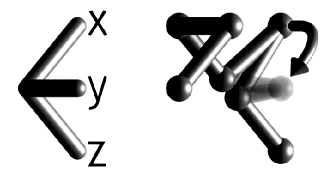
FIG. 2.: One elementary move of a monomer: a ‘kink’ (pair of anti-parallel neighbouring bonds) is replaced by another one.

FIG. 3.: Velocity of polymers of lengths $3$ up to $200$ in electric fields between $0.001$ and $1$. The velocity is plotted on the vertical logarithmic axis. On the horizontal logarithmic axis the electric field $E$ is plotted.

FIG. 4.: The position of the center of mass of a polymer of length $100$ divided by the electric field for the electric fields $0.1$, $0.03$, $0.01$, and $0.003$. The lines are the expected positions using the average speed measured by the long experiments.

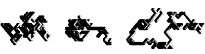
FIG. 5.: Three polymers of length $100$ in different electric fields. From left to right: $E=0.003$, $E=0.01$, $E=0.03$. Polymers in small electric fields look like random walks. In slightly larger electric fields the ends tend to protrude. In high electric fields the polymer does not look like a random walk.

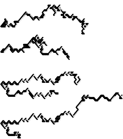
FIG. 6.: Four polymers of length $100$, and $E=0.1$. From top to bottom the times in Monte Carlo steps are: $5.8\cdot 10^{7}$, $8.6\cdot 10^{7}$, $1.25\cdot 10^{8}$ and $1.66\cdot 10^{8}$.

FIG. 7.: The average number of kinks on monomer number. The polymers are of length $100$ and electric fields are $0.003$, $0.01$, $0.03$ and $0.1$. The line gives the expected value $1/6$ of kinks in a random walk.

FIG. 8.: Transition between the linear and quadratic dependence of the velocity on the electric field. For various polymer lengths, the scaled velocity $v^{\prime}=(\sqrt{b}/a)v$ is plotted as a function of scaled electric field $E^{\prime}=(\sqrt{b/a})E$, where $a$ and $b$ are $L$-dependent parameters given in table II. The curve is given by $v^{\prime}=\sqrt{{E^{\prime}}^{2}+{E^{\prime}}^{4}}$.

FIG. 9.: Diffusion constant calculated from our measurements, compared to the scaling relation found by Barkema and Krenzlin. This scaling relation is a straight line when $N^{2}D$ is plotted as a function of $N^{-2/3}$.

TABLE I.: Encoding of a bond in three bits, where $x^{(i)}$ is the $i^{\mbox{th}}$ bit of $x$ and so on. Note that the encoding of the negative bonds is the binary complement of the positive bonds.

bond	$x^{(i)}$	$y^{(i)}$	$z^{(i)}$
+x	$1$	$0$	$0$
+y	$0$	$1$	$0$
+z	$0$	$0$	$1$
-x	$0$	$1$	$1$
-y	$1$	$0$	$1$
-z	$1$	$1$	$0$

TABLE II.: Values for $a$ and $b$, obtained by fitting the drift velocity to the form $v^{2}=aE^{2}+bE^{4}$; these values are used for scaling in figure 8. For large $L$ the parameter $a$ decreases quadratically with $L$ and $b$ is more or less constant. The graphs of $L^{2}a$ and $b$ show evidence of convergence to a constant; this is in agreement with Equation (12).

$L$	$a$	$b$
30	$1.85(6)\cdot 10^{-4}$	$1.9(2)\cdot 10^{-2}$
50	$4.4(2)\cdot 10^{-5}$	$5.5(2)\cdot 10^{-2}$
70	$1.79(5)\cdot 10^{-5}$	$8.3(2)\cdot 10^{-2}$
100	$7.32(7)\cdot 10^{-6}$	$1.12(1)\cdot 10^{-1}$
140	$3.31(3)\cdot 10^{-6}$	$1.29(1)\cdot 10^{-1}$
200	$1.5(1)\cdot 10^{-6}$	$1.4(7)\cdot 10^{-1}$

REFERENCES

- [1] To whom correspondence should be addressed.
- [2] P.G. de Gennes, J. Chem. Phys. 55, 572 (1972).
- [3] M. Rubinstein, Phys. Rev. Lett. 59, 1946 (1987).
- [4] K.E. Evans and S.F. Edwards, J. Chem. Soc. Faraday Trans. 2, 77, 1891-1912 (1981).
- [5] M. Prähofer and H. Spohn, Physica A 233, 191 (1996).
- [6] M.E.J. Newman and G.T. Barkema, Phys. Rev. E 56, 3468 (1997); G.T. Barkema and M.E.J. Newman, Physica A 244, 25-39 (1997).
- [7] T.A.J. Duke, Phys. Rev. Lett. 62, 2877 (1989).
- [8] G.T. Barkema, J.F. Marko and B. Widom, Phys. Rev. E 49, 5303 (1994).
- [9] A. van Heukelum, G.T. Barkema and R.H. Bisseling, to be published.
- [10] J.M. Deutsch and T.L. Madden, J. Chem. Phys. 91, 3252 (1989).
- [11] G.T. Barkema and H.M. Krenzlin, J. Chem. Phys. 109, 6486 (1998).
- [12] M. Widom and I. Al-Lehyani, Physica A 244, 510 (1997).
- [13] J.M. Deutsch and T.L. Madden, J. Chem. Phys. 90, 2476 (1989).
- [14] G.T. Barkema, C. Caron and J.F. Marko, Biopolymers 38, 665-667 (1996).
- [15] C. Heller, T.A.J. Duke and J.L. Viovy, Biopolymers 34, 249-259 (1994).
- [16] H. Hervet and C.P. Bean, Biopolymers 26, 727-742 (1987).