Spectral Properties of Random Reactance Networks and Random Matrix Pencils

Abstract

Our goal is to study statistical properies of ”dielectric resonances” which are poles of conductance of a large random $LC$ network. Such poles are a particular example of eigenvalues $\lambda_{n}$ of matrix pencils ${\bf H}-\lambda{\bf W}$, with ${\bf W}$ being a positive definite matrix and ${\bf H}$ a random real symmetric one. We first consider spectra of the matrix pencils with independent, identically distributed entries of ${\bf H}$. Then we concentrate on an infinite-range (”full-connectivity”) version of random $LC$ network. In all cases we calculate the mean eigenvalue density and the two-point correlation function in the framework of Efetov’s supersymmetry approach. Fluctuations in spectra turn out to be the same as those provided by the Wigner-Dyson theory of usual random matrices.

I Introduction

Large random reactance networks (that is networks made of random mixture of capacitances $C$ and inductances $L$) possess a peculiar property noticed first by Dykhne [1]: they have a finite real conductance and thus can disperse an electric power. Explanation of this somewhat paradoxical property is simple, however. Indeed, if such a network is large enough there always exist circuits of ”resonance type”, with (purely imaginary) conductance showing poles at some frequencies. Then the real part of the conductance as a function of frequency consists of a set of $\delta-$like peaks at those resonance frequencies. When the volume of the network grows to infinity, this set becomes more and more dense. Then, adding an arbitrary small (infinitesemal, but fixed) active part to all inductances ( one may think, e.g. of the inductance $L$ on each bond being in series with a weak resistance R) results in a finite active resistance of the network.

A random mixture of two active conductances is very well studied in correspondence with the bond percolation problem, see e.g.[2]. At the same time, the random reactance networks are relatively less studied.

It is necessary to mention that the random $LC$ (more generally, $RL-C$) networks emerge in various physical contexts. As was shown long ago by Shender[3] the conductance of the random $LC$ network turns out to be intimately related to properties of collective excitations in spin glasses. The mapping between the two problems is possible by an analogy noticed first by Kirkpatrick [4] between the Kirchhoff’s law and the equation of motion for the spin operators.

More recently, $RL-C$ networks were claimed to be an adequate model for describing the optical absorption in disordered metal films, see [5] and references therein, which showed some unusual features. This fact motivated Luck and collaborators for a series of insightful numerical investigations of two-dimensional $RL-C$ arrays [6, 7].

Since it is the conductance poles (resonances) of the $LC$ networks which dominate properties of the weakly dissipative $RL-C$ networks, it is natural to try to understand their properties in a greater detail. To access those poles it is convenient, following [7, 8] to start with the Kirchhoff equations for the electric potential at vertices $i$ of a network:

$$\sum_{j}\sigma_{ij}(V_{i}-V_{j})=0$$ (1)

where the summation goes over all vertices $j$ which are neighbours of a given $i$. The equations Eqs.(1) should be complimented with boundary conditions at electrodes. For a two-terminal geometry one assumes $V_{i}=0$ (resp. $V_{i}=V$) for the vertices $i$ belonging to the left (resp. right) terminal.

It is useful to introduce the (positive semidefinite) Laplace operator ${\bf D}$ on the network by

$$({\bf D}V)_{i}=\sum_{j}(V_{j}-V_{i})$$ (2)

with a convention $V_{i}=0$ on both electrodes.

In a random $LC$ network each conductance at frequency $f=\omega/2\pi$ is equal to either $\sigma_{0}=iC\omega$ or $\sigma_{1}=(iL\omega)^{-1}$, with a specified probabilities (in what follows we concentrate on the case of equal probability for finding $L$ and $C$ bonds in the network). Then the Laplace operator can be written as a sum $\bf{D}_{C}+{\bf D}_{L}$ of its components on the $L-$ and $C-$ bond sets, respectively. It is easy to show that the poles of the conductance occur at frequencies $f$ given by the roots of the equation [7, 8]:

$$\det{\left({\bf D}_{L}-\lambda{\bf D}\right)}=0$$ (3)

where we introduce the ratio

$$\lambda=\frac{\sigma_{0}}{\sigma_{0}-\sigma_{1}}=\frac{(\omega/\omega_{0})^{2}}{1+(\omega/\omega_{0})^{2}}\quad;\quad 0\leq\lambda\leq 1$$ (4)

with $\omega_{0}=1/(LC)^{1/2}$ being a characteristic resonant frequency of the LC network.

The simplest, but very informative way to understand properties of the random binary mixtures on average is to write an equation for the mean conductance $\Sigma$ using an effective-medium approximation (EMA). For a network with a coordination number $z$ and equal concentrations of $\sigma_{0}-$ and $\sigma_{1}-$bonds it reads as follows[4]:

$$\frac{\Sigma-\sigma_{0}}{2\sigma_{0}+(z-2)\Sigma}+\frac{\Sigma-\sigma_{1}}{2\sigma_{1}+(z-2)\Sigma}=0$$ (5)

Analysing the solution of this quadratic equation as a function of $\lambda$ in the interval $0\leq\lambda\leq 1$, one finds that generically for $z>4$ the real part of $\Sigma(\lambda)$ is non-zero only inside some interval $\lambda_{min}(z)\leq\lambda\leq\lambda_{max}(z)$. According to the discussion above it means that a mean density of resonances is finite only inside that interval.

Useful and simple as it is, EMA suffers from an essential drawback: it systematically neglects fluctuations, whereas taking the fluctuations into account could be important. For example, as was noted in [3, 7] the existence of sharp edges $\lambda_{min,max}$ was an artifact of the EMA approximation. In fact, the density of the resonances is never exactly zero inside the whole interval $\lambda\in[0,1]$ due to the so called Lifshitz tails, which is a purely fluctuation phenomenon. Apart from that, it seems hard to construct EMA as a systematic approximation with respect to some small parameter, though there are indications that it becomes progressively exact for higher spatial dimensions $d$ [9] and can be an extremely well-working one for many realistic systems [4]. Therefore, it is not clear how to correct it systematically or to include fluctuation effects into account.

These unsatisfactory features should be contrasted with the status of the mean-field approximation in the theory of magnetism, with which EMA shares its main ingredients. As is well known, the mean-field equations become exact for the model with the infinite range of spin interaction. Even for strongly disordered spin systems like spin glasses the latter model provides an adequate basis for constructing a mean-field theory with many non-trivial properties[10].

It is natural to try to consider a model of similar type also for the disordered reactance networks. This just amounts to considering the Kirchhoff equations Eqs.(1) on a disordered full-connectivity graph of $N$ vertices (nodes) connected by $N(N-1)/2$ edges (bonds), each independently taking a value $\sigma_{0}$ or $\sigma_{1}$.

Actually, we find it convenient to consider a graph with $N+2$ nodes, among them two ”terminal” nodes (labeled $A$ and $B$, respectively) are singled out by being attached to external voltage, so that the potential at $A$ is equal to $V$, whereas the potential at $B$ is kept zero. The rest of $N$ ”internal” nodes are labeled by index $i=1,...,N$ and the corresponding (induced) potentials are denoted with $V_{i}$. The nodes are connected in a full-connectivity graph of $(N+2)(N+1)/2-1$ bonds, with a single bond being excluded by obvious reasons: that connecting terminals $A$ and $B$ directly, see Fig.1.

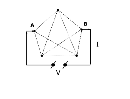
FIG. 1.: Schematic view of the full-connectivity graph with three internal nodes. One direct bond connecting the terminal nodes $A$ and $B$ is excluded.

We then attribute conductances $\sigma_{\mu\nu}=\sigma_{\nu\mu},\,\,\mu,\nu=A,B,1,...,N$ to each bond. It is convenient to introduce three $N-$ component vectors: $\underline{v}=(V_{1},...,V_{N})^{T},\,\,\underline{\sigma}_{A}=(\sigma_{A1},...,\sigma_{AN})^{T},\,\,\underline{\sigma}_{B}=(\sigma_{B1},...,\sigma_{BN})^{T}$ (we used here $T$ to indicate the transposition) and $N\times N$ matrix ${\bf\Sigma}$ with the following structure:

$\displaystyle{\bf\Sigma}=\left(\begin{array}[]{cccc}\sigma_{A1}+\sigma_{B1}+\sum_{k\neq 1}^{N}\sigma_{1k}&-\sigma_{12}&...&-\sigma_{1N}\\ -\sigma_{21}&\sigma_{A2}+\sigma_{B2}+\sum_{k\neq 2}^{N}\sigma_{2k}&...&-\sigma_{2N}\\ ...&...&...&...\\ -\sigma_{N1}&-\sigma_{N2}&...&\sigma_{AN}+\sigma_{BN}+\sum_{k\neq N}\sigma_{Nk}\end{array}\right)$

In these notations $N+1$ Kirchhof’s equations Eq.(1) ($N$ for the internal nodes $i$ and one for the node $B$) can be written, respectively:

$${\bf\Sigma}\underline{v}=V\underline{\sigma}_{A}\quad,\quad\underline{\sigma}^{T}_{B}\underline{v}=I$$ (6)

where $I$ stands for the total current flowing outwards through the terminal node $B$. This system of equations can be readily solved yielding the expression for the network conductance:

$$Y_{AB}=\frac{I}{V}=\underline{\sigma}^{T}_{B}{\bf\Sigma}^{-1}\underline{\sigma}_{A}$$ (7)

If we now deal with a binary networks when each $\sigma_{ij}$ is $\sigma_{0}$ with a probability $p$ and $\sigma_{1}$ with the probability $1-p$ it is convenient to introduce the ”symmetric” variables $h_{ij}$ such that $h_{ij}=-1$ if $\sigma_{ij}=\sigma_{0}$ and $h_{ij}=1$ if $\sigma_{ij}=\sigma_{1}$, so that $\sigma_{ij}=\frac{1}{2}\left([\sigma_{0}+\sigma_{1}]+[\sigma_{1}-\sigma_{0}]h_{ij}\right)$. In terms of these variables the network conductance Eq.(7) can be written as:

$$y_{ab}=Y_{AB}/\sigma_{0}=-\frac{1}{2\lambda}\left[\underline{h}_{B}^{T}-\tilde{\lambda}\underline{e}^{T}\right]\frac{1}{{\bf H}-\tilde{\lambda}{\bf W}}\left[\underline{h}_{A}-\tilde{\lambda}\underline{e}\right]$$ (8)

where $\tilde{\lambda}=2\lambda-1,\quad\underline{e}^{T}=(1,1,...,1),\quad\underline{h}_{B}^{T}=(h_{B1},...,h_{BN})$ and $N\times N$ matrices ${\bf W,H}$ have the following elements:

$$W_{ij}=(N+2)\delta_{ij}-1\quad,\quad H_{ij}=\delta_{ij}\left(h_{Ai}+h_{iB}+\sum_{k\neq i}h_{ik}\right)-(1-\delta_{ij})h_{ij}$$ (9)

With these expressions in hand we see that resonances of our network are determined by values of $\tilde{\lambda}$ satisfying the condition:

$$\det\left({\bf H}-\tilde{\lambda}{\bf W}\right)=0$$ (10)

Of course, it is evident that the full-connectivity construction would be completely inadequate one for describing the percolation problem which dominates properties of binary mixtures of two real conductances. We are, however, interested in studying the resonances of disordered LC networks, and the existence of such resonances is in no way precluded by ”all-to-all” geometry. We will find, that such a model turns out to be, in essence, exactly soluable in the limit $N\gg 1$. We start with deriving the mean density of resonances which turns out to be a function of the scaled variable $r=\tilde{\lambda}N^{1/2}$. One can envisage such a scaling already from the EMA result Eq.(5), which for $z\gg 1$ gives $|\lambda_{min,max}-1/2|\propto\tilde{\lambda}_{min,max}\sim z^{-1/2}$. At the same time, in contrast to EMA the support of the spectrum in the infinite-range model does not have artificial sharp edges $\tilde{\lambda}_{min,max}$, but rather the mean spectral density $\rho(r)$ smoothly decays to zero as long as $r\to\infty$ as $\rho(r)\propto e^{-r^{2}/2}$.

More interesting is the fact, that the infinite-range model opens a possibility to study fluctuations of various quantities. In the present paper we concentrate on spectral fluctuations and, correspondingly, study the two-point correlation function of the resonance densities. The latter turns out to be essentially the same as given by the famous Wigner-Dyson theory of random matrix spectra. This fact favourably agrees with overall numerical results [7] for the resonance spectra of two-dimensional disordered $LC$ networks. An origin of relatively small, but noticable deviations from the Wigner-Dyson statistics detected in [7] remains unclear for us at the moment and could be related to $2D$ features of the networks studied there which are not captured adequately by our infinite-ranged model. This issue deserves further investigations.

Actually, finding the set of $\lambda$’s satisfing Eq.(3) or Eq.(10) is an example of the generalized eigenvalue problem. The combination of matrices ${\bf D}_{L}-\lambda{\bf D}$ or ${\bf H}-\tilde{\lambda}{\bf W}$ in this respect is known in the mathematical literature as a pencil of matrices[11] or just the matrix pencil. Theory of the matrix pencils has many important applications such as e.g. vibration and bifurcation analysis in complicated structures [12] and game theory[13].

At the same time, it seems that the present knowledge on statistical properties of generalized eigenvalues of the pencils of random matrices is rather scarce. The paper [14] considers the mean number and the density of real eigenvalues for a pencil ${\bf H}-\lambda{\bf W}$, with both ${\bf H}$ and ${\bf W}$ being matrices with all independent real entries and no symmetry conditions imposed. At the same time, our original physical problem motivates us to be interested in the pencils formed by real symmetric matrices ${\bf H},{\bf W}$, with ${\bf W}$ being positive definite. It is clear that ${\bf W}>0$ ensures all the eigenvalues of the matrix pencils to be real (such pencils are sometimes called in the literature the regular ones [11]). Indeed, in that case the generalized eigenproblem: ${\bf H}\underline{x}=\lambda{\bf W}\underline{x}$ is equivalent to a usual one: ${\bf W}^{-1/2}{\bf H}{\bf W}^{-1/2}\underline{y}=\lambda\underline{y}\quad,\quad\underline{y}={\bf W}^{1/2}\underline{x}$, with $\tilde{\bf H}={\bf W}^{-1/2}{\bf H}{\bf W}^{-1/2}$ being a real symmetric matrix.

The mean eigenvalue density for matrices of similar types (when both ${\bf W}$ and ${\bf H}$ are random) was studied in some generality starting from the work by Marchenko and Pastur, see [15]. In fact, the mean eigenvalue density can be found for the ensemble $\tilde{\bf H}$, with ${\bf H}$ being a real symmetric matrix with independent, identically distributed (i.i.d.) entries using a generalized version of results by Pastur[16]. We are however not aware of any systematic study of spectral correlations of regular pencils of the random matrices.

This should be contrasted with a very intensive research on eigenvalues of the random matrices (which is a particular case of ${\bf W}\equiv{\bf 1}$) performed in recent years in the domain of theoretical and mathematical physics[17]. Below we summarize the most important facts known from these studies.

As is well established [18, 19, 20, 22, 23], the statistical properties of real eigenvalues $X_{i}$ of large $N\times N$ self-adjoint random matrices ${\bf H}$ are to large extent universal, i.e. independent of the details of the distributions ${\cal P}({\bf H})$ of their entries.

It is important to mention the existence, in general, of two different characteristic scales in the random matrix spectra: the global one and the local one. The global scale is that on which the eigenvalue density, defined as $\rho(X)=\frac{1}{N}\mbox{Tr}\delta(X-{\bf H})$, changes appreciably with its argument $X$ when averaged over ${\cal P}({\bf H})$. For matrices whose spectrum has a finite support in the interval $X\in[A,B]$ the global scale is just the length of this interval.

In contrast, the local scale is that determined by the typical separation $\Delta=\langle X_{i}-X_{i-1}\rangle$ between neighbouring eigenvalues situated around a point $X$, with the brackets standing for the statistical averaging. It is given therefore by $\Delta=(\langle N\rho(X)\rangle)^{-1}$. If we are interested in those values of $X$ that are sufficiently far from the edges of the spectra the global scale is , roughly speaking, by a factor of $N$ larger than the local one. In other words, the mean density $\langle\rho(X)\rangle$ can be considered as a constant one on the scale $\Delta$.

The degree of universality is essentially dependent on the chosen scale.

As to the global scale universality, one can mention first of all that for the matrices with i.i.d. entries under quite general conditions (see, e.g., [24] and references therein) the mean density is given in the limit $N\to\infty$ by the so-called ”Wigner semicircle law”:

$$\langle\rho(X)\rangle=\frac{1}{2\pi a^{2}}\sqrt{4\,a^{2}-X^{2}}=\frac{1}{N\Delta}$$ (11)

In this expression the parameter $a$ just sets the global scale in the sense defined above. It is determined by the expectation value $a^{2}=\langle\frac{1}{N}Tr{\bf H}^{2}\rangle$. It is generally accepted to scale the entries $H_{ij}\sim 1/N^{1/2}$, i.e. in such a way that $a$ stays finite when $N\to\infty$, the local spacing between eigenvalues in the neighbourhood of the point $X$ being therefore $\Delta\propto 1/N$.

From the point of view of universality the semicircular eigenvalue density is not extremely robust. Most easily one violates it by considering an important class of the so-called ”invariant ensembles” characterized by a probability density of the form ${\cal P}({\bf H})\propto\exp{-NTrV({\bf H})}$, with $V({\bf H})$ being an even polynomial. The corresponding eigenvalue density turns out to be highly nonuniversal and is determined by the particular form of the potential $V(H)$. Only for $V({\bf H})={\bf H}^{2}$ it is given by the semicircular law, Eq.(11). Actually, any “deformation” ${\bf H}_{1}={\bf H}_{0}+{\bf H}$ of the ensemble ${\bf H}$ with i.i.d. entries by a given fixed matrix ${\bf H}_{0}$ results in the mean eigenvalue density belonging to a family of “deformed semicircular laws” discovered by Pastur[16].

Moreover, one can easily have a non-semicircular eigenvalue density even for real symmetric matrices ${\bf S};\quad S_{ij}=S_{ji}$ with i.i.d. entries, if one keeps the mean number of non-zero entries $p$ per column to be of the order of unity when performing the limit $N\to\infty$. This is a characteristic feature of the so-called sparse random matrices[22, 25, 26] characterized by the following probability density of a given entry $S_{ij}$ :

$${\cal P}(S_{ij})=(1-\frac{p}{N})\delta(S_{ij})+\frac{p}{N}h(S_{ij})$$ (12)

where $h(s)=h(-s)$ is an arbitrary even distribution function satisfying the conditions: $h(0)<\infty;\quad\int h(s)s^{2}ds<\infty$.

Remarkably, a much more profound universality emerges for the two-point correlation spectral function defined as:

$$\left\langle\rho(X_{1})\rho(X_{2})\right\rangle_{c}=\left\langle\rho(X_{1})\right\rangle\delta(X_{1}-X_{2})-{\cal Y}_{2}(X_{1},X_{2}),$$ (13)

where we defined the connected part of the correlation function in a usual manner: $\langle AB\rangle_{c}=\langle AB\rangle-\langle A\rangle\langle B\rangle$. The nontrivial part of the spectral correlator is called the cluster function ${\cal Y}_{2}(X_{1},X_{2})$. It is one of the most informative statistical measures of the spectra, [28]. It turns out, that already the global scale behaviour of ${\cal Y}_{2}(X_{1},X_{2})$ (i.e. one for the distance $S$ being comparable with the support of the spectrum in the limit $N\to\infty$) is rather universal. It is the same for all the ”invariant ensembles” [19] and for those with i.i.d. matrix elements[23] and is determined only by the positions of edge points $[A,B]$ of the spectrum [27].

Even more interesting is the fact that universality of the correlation function Eq.(13) (as well as of all higher correlation functions) extends to the local scale, i.e. for the distances $|X_{1}-X_{2}|$ comparable with $\Delta$. This fact was rigorously proved for the unitary invariant ensembles[18], extended to the unitary “deformed” ensembles[21] and heuristically verified for other invariant ensembles[20] as well as for the ensembles of sparse matrices[22, 29]. The particular form of the cluster function is different from that typical for the global scale. It is dictated in general by global symmetries of the random matrices, e.g.if they are complex Hermitian or real symmetric [28]. All specific (nonuniversal) properties are encoded in the value of local spacing $\Delta$. For the distances $S$ such that $S\gg\Delta$ local expressions match with the global one, the latter taken at distances $S\ll[A-B]$.

It turns out, that it is the local scale universality that is mostly relevant for real physical systems[30]. Namely, the statistics of highly excited bound states of closed quantum chaotic systems of quite different microscopic nature turn out to be independent of the microscopic details when sampled on the energy intervals large in comparison with the mean level separation, but smaller than the energy scale related by the Heisenberg uncertainty principle to the relaxation time necessary for a classically chaotic system to reach equilibrium in phase space [31]. Moreover, the spectral correlation functions turn out to be exactly those which are provided by the theory of large random matrices on the local scale [32, 33], with different symmetry classes corresponding to presence or absence of the time-reversal symmetry.

Motivated by lack of general theoretical results for spectral properties of the pencils of random matrices, we start in Sec.II with considering an abstract pencil , with real symmetric ${\bf H}$ belonging to the Gaussian ensemble of random matrices with i.i.d. entries and $W$ being a real symmetric positive definite one with fixed given entries. We derive an expression for the mean spectral density of such a pencil and demonstrate that the correlation properties on the local scale (in the sense defined above) are the same as given by the Wigner-Dyson expressions. Then, in Sec.III we extend our consideration to the case of resonance statistics in the random infinite-range LC-network, by deriving the mean density and the two-point spectral correlation function for the resonances.

II Wigner-Dyson universality for spectra of regular matrix pencils

To study spectral properties of a regular matrix pencil ${\bf H}-\lambda{\bf W}$ we employ the Efetov supersymmetry approach [34, 35]. A pedestrian introduction into the method can be found in [36].

A convenient starting point is a representation of the spectral density $\rho(\lambda)$ of real eigenvalues $\lambda_{n}$ for the equivalent symmetric eigenvalue problem for the matrix $\tilde{\bf H}={\bf W}^{-1/2}{\bf H}{\bf W}^{-1/2}$ in the following form:

$$\rho(\lambda)=\frac{1}{N}\sum_{n=1}^{N}\delta(\lambda-\lambda_{n})=\mp\lim_{\epsilon\to+0}\frac{1}{\pi N}\mathop{\mathrm{Im}}\mathop{\mathrm{Tr}}\frac{1}{(\lambda\pm i\epsilon){\bf 1}-\tilde{\bf H}}$$ (14)

which after a trivial manipulation can be rewritten as a derivative

$$\rho(\lambda)=\mp\mathop{\mathrm{Im}}\frac{1}{\pi N}\lim_{\epsilon\to+0}\lim_{J\to 0}\frac{\partial}{\partial J}{\cal Z}_{\pm}(J,\lambda)$$ (15)

of a generation function ${\cal Z}_{\pm}(J,\lambda)$ defined as

$${\cal Z}_{\pm}(J,\lambda)=\frac{\det\left[(\lambda\pm i\epsilon+J){\bf W}-{\bf H}\right]}{\det\left[(\lambda\pm i\epsilon){\bf W}-{\bf H}\right]}$$ (16)

In a completely analogous way one expresses the two-point spectral correlation function (”cluster function”, see Eq.(13)):

$$-{\cal Y}_{2}(\lambda_{1},\lambda_{2})=\langle\rho(\lambda_{1})\rho(\lambda_{2})\rangle-\langle\rho(\lambda_{1})\rangle\langle\rho(\lambda_{2})\rangle=\frac{1}{2\pi^{2}}\mathop{\mathrm{Re}}{\cal K}_{con}(\lambda_{1},\lambda_{2})$$ (17)

as

$${\cal K}_{con}(\lambda_{1},\lambda_{2})=\frac{1}{N^{2}}\lim_{\epsilon\to+0}\lim_{J_{1,2}\to 0}\frac{\partial^{2}}{\partial J_{1}\partial J_{2}}\left[\langle{\cal Z}_{-}(J_{1},\lambda_{1}){\cal Z}_{+}(J_{2},\lambda_{2})\rangle-\langle{\cal Z}_{-}(J_{1},\lambda_{1})\rangle\langle{\cal Z}_{+}(J_{2},\lambda_{2})\rangle\right]$$ (18)

where the angular brackets stand for the ensemble averaging and we assume that $\lambda_{1}\neq\lambda_{2}$. The expressions above are actually valid in the limit $N\to\infty$, where one can show that

$$\lim_{\epsilon\to+0}\lim_{J_{1,2}\to 0}\frac{\partial^{2}}{\partial J_{1}\partial J_{2}}\left[\langle{\cal Z}_{\pm}(J_{1},\lambda_{1}){\cal Z}_{\pm}(J_{2},\lambda_{2})\rangle-\langle{\cal Z}_{\pm}(J_{1},\lambda_{1})\rangle\langle{\cal Z}_{\pm}(J_{2},\lambda_{2})\rangle\right]=0$$

and we used this fact in Eq.(17).

To facilitate the ensemble averaging we represent the ratio of the two determinants in Eq.(16) as the Gaussian integral

$${\cal Z}_{\pm}(J,\lambda)=(-1)^{N}\int\prod_{i=1}^{N}[d\Psi_{i}(\pm)]\exp\{\pm\frac{i}{2}\sum_{i,j}^{N}\Psi_{i}^{\dagger}(\pm)\left[W_{ij}(\lambda\pm i\epsilon+J\hat{k})-H_{ij}\right]\Psi_{j}(\pm)\}$$ (19)

over 4-component supervectors $\Psi_{i}(\pm)$,

$$\Psi_{i}(\pm)=\left(\begin{array}[]{c}\vec{R}_{i}(\pm)\\ \vec{\eta}_{i}(\pm)\end{array}\right),\vec{R}_{i}(\pm)=\left(\begin{array}[]{c}r_{i}(\pm)\\ r_{i}^{*}(\pm)\end{array}\right),\vec{\eta}_{i}(\pm)=\left(\begin{array}[]{c}\chi_{i}(\pm)\\ \chi_{i}^{*}(\pm)\end{array}\right),d\Psi_{i}=\frac{dr_{i}dr_{i}^{*}}{2\pi}d\chi_{i}^{*}d\chi_{i}$$ (20)

with the components $r_{i}(+),r_{i}(-);\quad i=1,2,...,N$ being complex commuting variables and $\chi_{i}(+),\chi_{i}(-)$ forming the corresponding Grassmannian parts of the supervectors $\Psi_{i}(\pm)$. A $4\times 4$ diagonal supermatrix $\hat{k}=\mathop{\mathrm{diag}}(0,0,1,1)$ takes care of absence of the source $J$ in the denomenator of the generating function Eq(16).

Since we are dealing finally with the averaged product of two such generating functions it is convenient to introduce the $8-$component supervectors

$$\Phi_{i}=\left(\begin{array}[]{c}\Psi_{i}(+)\\ \Psi_{i}(-)\end{array}\right)$$ (21)

and finally $\Phi=\left(\Phi_{1},...,\Phi_{N}\right)^{T}$ as well as the supermatrices $\hat{\Lambda}=\mathop{\mathrm{diag}}(1,1,1,1,-1,-1,-1,-1)$ and $\hat{J}_{k}=\mathop{\mathrm{diag}}(J_{1}\hat{k},J_{2}\hat{k})$.

It is also useful to remember that we expect to have non-trivial spectral correlations on the scale comparable with the mean spacing between neigbouring eigenvalues, i.e. when $\lambda_{1}-\lambda_{2}\propto 1/N$. Correspondingly, we introduce: $\lambda_{1}=\lambda-s/2N\quad,\quad\lambda_{2}=\lambda+s/2N$ and consider $s$ to be of the order of unity henceforth. All this allows us to write the product of two generating functions as

$${\cal Z}^{\lambda,s}(J_{1},J_{2})={\cal Z}_{-}(J_{1},\lambda_{1}){\cal Z}_{+}(J_{2},\lambda_{2})=$$ (22)

$$\int d\Phi\exp\left\{-\frac{i}{2}\Phi^{\dagger}\hat{\Lambda}\otimes{\bf H}\Phi+\frac{i}{2}\Phi^{\dagger}\left[\lambda\hat{\Lambda}-(\epsilon-is/2N)\hat{1}+\hat{J}_{k}\right]\otimes{\bf W}\Phi\right\}$$ (23)

This expression can be easily averaged over the Gaussian distribution of ${\bf H}$ by the chain of identities:

$$\left\langle e^{-\frac{i}{2}\Phi^{\dagger}\hat{\Lambda}\otimes{\bf H}\Phi}\right\rangle=e^{-\frac{a^{2}}{4N}\mathop{\mathrm{Str}}\hat{A}^{2}}=\int d\hat{Q}\exp{\left[-\frac{N}{4}\mathop{\mathrm{Str}}\hat{Q}^{2}-i\frac{a}{2}\Phi^{\dagger}\hat{\Lambda}\hat{Q}\Phi\right]}$$ (24)

where $a$ determines the variance of matrix elements of ${\bf H}$, see Eq.(11) and $\hat{A}=\hat{\Lambda}^{1/2}\left(\sum_{i}\Phi_{i}\otimes\Phi^{\dagger}\right)\hat{\Lambda}^{1/2}$. The last relation trading the term in the exponent quartic with respect to $\Phi$ for an auxilliary integration over the set of supermatrices $\hat{Q}$ is known as the Hubbard-Stratonovich transformation and plays a cornerstone role in the whole method. After substituting Eq.(24) back into averaged Eq.(22) and changing the order of integrations one performs the (Gaussian) integral over $\Phi$ explicitly. It turns out that in order to justify all these operations formally one has to restrict the supermatrices $\hat{Q}$ to a manifold paramatrized as $\hat{Q}=\hat{T}^{-1}\hat{P}\hat{T}$, with $\hat{P}$ being a block-diagonal Hermitian supermatrix and $\hat{T}$ belonging to a certain graded coset space $UOSP(2,2/4)/UOSP(2/2)\otimes UOSP(2/2)$. A detailed discussion of this fact and an explicit parametrisation of the matrices $\hat{T}$ could be found in [34, 35, 36, 37].

The resulting expression for the averaged product of the generation functions turns out to be dependent only on eigenvalues $w_{i}\,,\,i=1,...,N$ of the matrix ${\bf W}$ (this fact can be traced back to the ”rotational invariance” of the Gaussian Orthogonal Ensemble (GOE) formed by ${\bf H}$) and has the following form:

$$\langle{\cal Z}^{\lambda,s}(J_{1},J_{2})\rangle=\int d\hat{Q}\exp{\left[-\frac{N}{4}\mathop{\mathrm{Str}}\hat{Q}^{2}-\frac{1}{2}\sum_{i=1}^{N}\mathop{\mathrm{Str}}\ln\left\{\left(\lambda\hat{1}-v_{i}\hat{Q}\right)+\left(i\epsilon+s/2N+\hat{J}_{k}\right)\hat{\Lambda}\right\}\right]}$$ (25)

where $v_{i}=a/w_{i}$.

Since we are interested in the limit $(\epsilon,J,1/N)\to 0$, we can expand the logarithm in the exponent correspondingly:

$$\begin{array}[]{c}\mathop{\mathrm{Str}}\ln\left\{\left(\lambda\hat{1}-v_{i}\hat{Q}\right)+\left(i\epsilon+s/2N+\hat{J}_{k}\right)\hat{\Lambda}\right\}=\\ \mathop{\mathrm{Str}}\ln\left(\lambda\hat{1}-v_{i}\hat{Q}\right)+\mathop{\mathrm{Str}}\left(\lambda\hat{1}-v_{i}\hat{Q}\right)^{-1}\hat{\Lambda}\left(i\epsilon+s/2N+\hat{J}_{k}\right)-\frac{1}{2}\mathop{\mathrm{Str}}\left[\left(\lambda\hat{1}-v_{i}\hat{Q}\right)^{-1}\hat{\Lambda}\hat{J}_{k}\right]^{2}+...\end{array}$$ (26)

so that differentiating the exponent over the sources $J_{1,2}$ yields the preexponential factors:

$$\lim_{J_{1,2}\to 0}\frac{\partial}{\partial J_{1}}\exp\{...\}\propto\sum_{i=1}^{N}\mathop{\mathrm{Str}}\left[\left(\lambda\hat{1}-v_{i}\hat{Q}\right)^{-1}\hat{k}\frac{\hat{\Lambda}+\hat{1}}{2}\right]$$ (27)

and

$$\begin{array}[]{c}\lim_{J_{1,2}\to 0}\frac{\partial^{2}}{\partial J_{1}\partial J_{2}}\exp\{...\}\propto 2\sum_{i=1}^{N}\mathop{\mathrm{Str}}\left[\left(\lambda\hat{1}-v_{i}\hat{Q}\right)^{-1}\hat{k}\frac{\hat{\Lambda}+\hat{1}}{2}\left(\lambda\hat{1}-v_{i}\hat{Q}\right)^{-1}\hat{k}\frac{\hat{\Lambda}-\hat{1}}{2}\right]\\ +\sum_{i=1}^{N}\mathop{\mathrm{Str}}\left[\left(\lambda\hat{1}-v_{i}\hat{Q}\right)^{-1}\hat{k}\frac{\hat{\Lambda}+\hat{1}}{2}\right]\sum_{i=1}^{N}\mathop{\mathrm{Str}}\left[\left(\lambda\hat{1}-v_{i}\hat{Q}\right)^{-1}\hat{k}\frac{\hat{\Lambda}-\hat{1}}{2}\right]\end{array}$$ (28)

In the limit $N\gg 1$ each sum over $i$ is of the order of $N$, so that a contribution of second term in the expression above is by factor $N$ larger than the contribution of the first one. In other words, we could restrict ourselves by terms linear in sources $J_{1,2}$ in the expansion Eq.(26) above. We will make use of this fact later on when considering a more complicated situation in the next section.

Taking all this into account, we arrive at the following integral representation:

$${\cal K}(\lambda_{1},\lambda_{2}) = \frac{1}{N^{2}}\lim_{\epsilon\to+0}\lim_{J_{1,2}\to 0}\frac{\partial^{2}}{\partial J_{1}\partial J_{2}}\langle{\cal Z}_{-}(J_{1},\lambda_{1}){\cal Z}_{+}(J_{2},\lambda_{2})\rangle$$ (29)

$$= \frac{1}{4N^{2}}\lim{\epsilon\to 0}\int dQ\exp{\left[-N{\cal L}(\hat{Q})-\frac{i}{2}\left(\epsilon-is/2N\right)\sum_{i}\mathop{\mathrm{Str}}\left(\lambda\hat{1}-v_{i}\hat{Q}\right)^{-1}\hat{\Lambda}\right]}$$ (31)

$$\times\sum_{i=1}^{N}\mathop{\mathrm{Str}}\left[\left(\lambda\hat{1}-v_{i}\hat{Q}\right)^{-1}\hat{k}\frac{\hat{\Lambda}+\hat{1}}{2}\right]\sum_{i=1}^{N}\mathop{\mathrm{Str}}\left[\left(\lambda\hat{1}-v_{i}\hat{Q}\right)^{-1}\hat{k}\frac{\hat{\Lambda}-\hat{1}}{2}\right]$$

where

$${\cal L}(\hat{Q})=\frac{1}{2}\mathop{\mathrm{Str}}\hat{Q}^{2}+\frac{1}{N}\sum_{i}\mathop{\mathrm{Str}}\ln\left(\lambda\hat{1}-v_{i}\hat{Q}\right)$$ (32)

In the same way one obtains the expression for the mean spectral density:

$$\rho(\lambda)=\frac{1}{N\pi}\lim_{\epsilon\to 0}\mathop{\mathrm{Im}}\int dQ\sum_{i=1}^{N}\mathop{\mathrm{Str}}\left[\left(\lambda\hat{1}-v_{i}\hat{Q}\right)^{-1}\hat{k}\frac{\hat{\Lambda}+\hat{1}}{2}\right]\exp{\left[-N{\cal L}(\hat{Q})-\frac{i}{2}\epsilon\sum_{i}\mathop{\mathrm{Str}}\left(\lambda\hat{1}-v_{i}\hat{Q}\right)^{-1}\hat{\Lambda}\right]}$$ (33)

In the limit $N\to\infty$ the integrals over $\hat{Q}$ in the expressions above are dominated by saddle points of the ”action” ${\cal L}(\hat{Q})$ Eq.(32) which satisfy the equation:

$$\hat{Q}=\frac{1}{N}\sum_{i=1}^{N}\frac{v_{i}}{\lambda\hat{1}-v_{i}\hat{Q}}$$ (34)

relevant solutions of which belonging to the integration domains $\hat{Q}=\hat{T}^{-1}\hat{P}\hat{T}$ are parametrized as follows:

$$\hat{Q}_{s.p.}=t\hat{1}+iq\hat{T}^{-1}\hat{\Lambda}\hat{T}$$ (35)

where the real parameters $t,q$ satisfy for $q\neq 0$ the system of two equations:

$$t=\frac{1}{N}\sum_{i}\frac{v_{i}(\lambda-v_{i}t)}{(\lambda-v_{i}t)^{2}+q^{2}v_{i}^{2}}\quad\mbox{and}\quad 1=\frac{1}{N}\sum_{i}\frac{v_{i}^{2}}{(\lambda-v_{i}t)^{2}+q^{2}v_{i}^{2}}$$ (36)

Let us note, that the saddle-point solutions Eq.(35) form for $q\neq 0$ a continuos manifold parametrized by the supermatrices $\hat{T}$.

Using these expressions it is easy to invert the matrix $\left(\lambda\hat{1}-v_{i}\hat{Q}_{s.p}\right)$ and check that

$$\sum_{i=1}^{N}\mathop{\mathrm{Str}}\left[\left(\lambda\hat{1}-v_{i}\hat{Q}_{s.p}\right)^{-1}\hat{k}\frac{\hat{\Lambda}\pm\hat{1}}{2}\right] = \pm 2\frac{\lambda-v_{i}t}{(\lambda-v_{i}t)^{2}+q^{2}v_{i}^{2}}+iq\frac{v_{i}}{(\lambda-v_{i}t)^{2}+q^{2}v_{i}^{2}}\mathop{\mathrm{Str}}\left[\hat{T}^{-1}\hat{\Lambda}\hat{T}\hat{k}\frac{\hat{1}\pm\hat{\Lambda}}{2}\right]$$ (37)

$$\sum_{i}\mathop{\mathrm{Str}}\left(\lambda\hat{1}-v_{i}\hat{Q}_{s.p}\right)^{-1}\hat{\Lambda} = i\mathop{\mathrm{Str}}\left[\hat{T}^{-1}\hat{\Lambda}\hat{T}\hat{\Lambda}\right]\sum_{i}\frac{v_{i}q}{(\lambda-v_{i}t)^{2}+q^{2}v_{i}^{2}}$$ (38)

So the problem amounts to substituting these expressions into the integrand of Eqs.(29,33) and to performing the remaining integration over the coset space parametrized by the matrices $\hat{T}$. The way of doing it described in much detail in [34, 35, 36, 37] and we refer the interested reader to those papers.

Here we mention only a few most important moments. First of all the integral in Eq.(33) is given by the so-called PSEW (Parisi-Sourlas-Efetov-Wegner) theorem due to a specific symmetry of the integrand ( in the limit $\epsilon\to 0$ the integrand contains only a part of the integration variables due to the projector $(\hat{\Lambda}+1)/2$) The resulting mean eigenvalue density is merely given by:

$$\rho(\lambda)=\frac{q}{\pi N}\sum_{i}\frac{v_{i}}{(\lambda-v_{i}t)^{2}+q^{2}v_{i}^{2}}$$ (39)

The system of equations Eqs(36,39) turns out to be in fact equivalent to a particular case of general results by Pastur and Girko[16].

Substituting the expression Eq.(39) for the mean spectral density to Eqs.(37) and the resulting formulae further to the integral Eq.(29,32) for the averaged generating function one can express the ”connected” part of the two-point correlation function ${\cal K}_{con}(\lambda_{1},\lambda_{2})$ as:

$${\cal K}_{con}(\lambda_{1},\lambda_{2}) =$$ (40)

$$\frac{\pi^{2}\rho^{2}(\lambda)}{4} \int d\mu{(T)}\mathop{\mathrm{Str}}\left[\hat{T}^{-1}\hat{\Lambda}\hat{T}\hat{k}\frac{\hat{1}+\hat{\Lambda}}{2}\right]\mathop{\mathrm{Str}}\left[\hat{T}^{-1}\hat{\Lambda}\hat{T}\hat{k}\frac{\hat{1}-\hat{\Lambda}}{2}\right]\exp\left\{-\frac{i\pi\rho(\lambda)}{4}s\mathop{\mathrm{Str}}\left[\hat{T}^{-1}\hat{\Lambda}\hat{T}\hat{\Lambda}\right]\right\}$$ (41)

with $d\mu(T)$ being an appropriate invariant measure on the coset space. When deriving that expression from Eqs.(29,32,37) we noticed that the ”disconnected” part of the correlation function is again given by PSEW theorem and cancels exactly the contribution from those few terms in the integrand which are not proportional to the mean density $\rho(\lambda)$.

The expression Eq.(40) is our main result and is quite remarkable: its form exactly coincides with the corresponding expression for the two-point correlation function of random matrices from GOE, see e.g. [37]. This fact was first demonstrated by Efetov who managed to perform a non-trivial integration over the coset-space explicitly[34] and found that it reproduced the famous Dyson expression[38] for the two-point function[28]:

$${\cal Y}_{2}(\lambda_{1},\lambda_{2})=\left(\frac{\sin s_{e}}{s_{e}}\right)^{2}+\frac{d}{ds_{e}}\left(\frac{\sin s_{e}}{s_{e}}\right)\int_{1}^{\infty}dt\frac{\sin{(s_{e}t)}}{t}$$ (42)

where $s_{e}=\pi\rho(\lambda)s$ is a spectral distance $s/N$ measured in units of the local mean spacing $\Delta=1/[N\rho(\lambda)]$.

In the end of the present section we just mention that our method of deriving Eq.(40) can be easily generalized to matrix pencils whose random part ${\bf H}$ is an arbitrary matrix (real symmetric or Hermitian) with i.i.d. entries following the lines of papers[22, 26]. In the same way one can show that all higher correlation functions also coincide with GOE expressions.

III Spectral properties of a ”full connectivity” LC network

Now we are well-prepared to calculate the mean density of resonances and the corresponding two-point spectral correlation function of the ”full-connectivity” LC network as defined by eqs.(9,10). Actually, it is convenient to rescale both matrices in Eq.9 as: ${\bf H}\to\frac{1}{N^{1/2}}{\bf H},\quad{\bf W}\to\frac{1}{N^{1/2}}{\bf W}$. This transformation obviously does not change generalized eigenvalues of the pencil ${\bf H}-\tilde{\lambda}{\bf W}$ but facilitates bookkeeping of the leading terms in various expansions.

In our consideration we follow the pattern of the previous section and introduce the generation function identical to Eq.(22):

$${\cal Z}^{r,s}(J_{1},J_{2})=\int\prod_{i}d\Phi_{i}\exp\left\{-\frac{i}{2N^{1/2}}\sum_{i=1}^{N}\Phi_{i}^{\dagger}\left[(h_{Ai}+h_{Bi})\hat{\Lambda}-2i\tilde{\epsilon}\hat{1}-2\left(\frac{r}{N^{1/2}}\hat{\Lambda}+\hat{J}\right)\right]\Phi_{i}\right\}$$ (43)

$$\times\exp\left\{\frac{i}{2N^{1/2}}\sum_{i<j}^{N}\left(\Phi_{i}^{\dagger}-\Phi_{j}^{\dagger}\right)\left[\frac{r}{N^{1/2}}\hat{\Lambda}+\hat{J}_{k}+i\tilde{\epsilon}\hat{1}+h_{ij}\hat{\Lambda}\right]\left(\Phi_{i}-\Phi_{j}\right)\right\}$$ (44)

where we used that

$\displaystyle\frac{1}{2}\sum_{i<j}h_{ij}(\Phi_{i}^{\dagger}-\Phi_{j}^{\dagger})\hat{B}(\Phi_{i}-\Phi_{j})=-\sum_{i<j}h_{ij}\Phi_{i}^{\dagger}\hat{B}\Phi_{j}+\frac{1}{2}\sum_{i}\Phi_{i}^{\dagger}\hat{B}\Phi_{i}\left(\sum_{k\neq i}h_{ik}\right)$

for any supermatrix $\hat{B}$ as long as $\Phi_{i}^{\dagger}\hat{B}\Phi_{j}=\Phi_{j}^{\dagger}\hat{B}\Phi_{i}$. We also envisaged that for the full-connectivity network the resonance density is nonvanishing as long as $\tilde{\lambda}\sim 1/N^{1/2}$ and introduced the scaled variable $r=\tilde{\lambda}N^{1/2}$ (see the Introduction). Then the typical spacing between neighbouring resonances should be of the order of $\Delta\sim N^{-3/2}$. Since we can expect a nontrivial spectral correlation on the distances $S=\tilde{\lambda}_{2}-\tilde{\lambda}_{1}$ comparable with $\Delta$ we introduced the quantity $\tilde{\epsilon}=\epsilon-is/(2N^{3/2})$ and consider $s$ to be of the order of unity. All other notations coincide with those in Eq.(22).

Now we have to perform the averaging over $h_{\mu\nu},\,\,(\mu,\nu)=A,B,1,...,N$, each taking values $\pm 1$ with the equal probabilities. This is done in the limit $N\to\infty$ as follows:

$$\prod_{i<j}\left\langle\exp\left\{\frac{i}{2N^{1/2}}h_{ij}\left(\Phi_{i}^{\dagger}-\Phi_{j}^{\dagger}\right)\hat{B}\left(\Phi_{i}-\Phi_{j}\right)\right\}\right\rangle=$$ (45)

$$\prod_{i<j}\frac{1}{2}\left[\exp\left\{\frac{i}{2N^{1/2}}\left(\Phi_{i}^{\dagger}-\Phi_{j}^{\dagger}\right)\hat{B}\left(\Phi_{i}-\Phi_{j}\right)\right\}+\exp\left\{-\frac{i}{2N^{1/2}}\left(\Phi_{i}^{\dagger}-\Phi_{j}^{\dagger}\right)\hat{B}\left(\Phi_{i}-\Phi_{j}\right)\right\}\right]=$$ (46)

$$\prod_{i<j}\left\{1-\frac{1}{8N}\left[\left(\Phi_{i}^{\dagger}-\Phi_{j}^{\dagger}\right)\hat{B}\left(\Phi_{i}-\Phi_{j}\right)\right]^{2}+...\right\}\approx\exp\{-\frac{1}{16N}\sum_{i,j}\left[\left(\Phi_{i}^{\dagger}-\Phi_{j}^{\dagger}\right)\hat{B}\left(\Phi_{i}-\Phi_{j}\right)\right]^{2}\}$$ (47)

and in similar way we can average also over $h_{A,i},h_{B,i}$. Introducing now the notations:

$${\cal K}(\Phi_{a},\Phi_{b})=-4ir\left(\Phi_{a}^{\dagger}-\Phi_{b}^{\dagger}\right)\hat{\Lambda}\left(\Phi_{a}-\Phi_{b}\right)+\left[\left(\Phi_{a}^{\dagger}-\Phi_{b}^{\dagger}\right)\hat{\Lambda}\left(\Phi_{a}-\Phi_{b}\right)\right]^{2}$$ (48)

$$f(\Phi)=\frac{i}{N^{1/2}}\Phi^{\dagger}\left(i\tilde{\epsilon}\hat{1}+\frac{r}{N^{1/2}}\hat{\Lambda}+\hat{J}_{k}\right)\Phi-\frac{1}{4N}\left(\Phi^{\dagger}\hat{\Lambda}\Phi\right)^{2}$$ (49)

we can rewrite the averaged generating function as:

$${\cal Z}(J_{1},J_{2})_{av} = \int\prod_{i}d\Phi_{i}\exp\left\{\sum_{i}f(\Phi_{i})-\frac{1}{16N}\sum_{ij}{\cal K}(\Phi_{i},\Phi_{j})\right\}$$ (51)

$$\times\exp\left\{\frac{i}{2N^{1/2}}\sum_{i<j}\left(\Phi_{i}^{\dagger}-\Phi_{j}^{\dagger}\right)\left[i\tilde{\epsilon}\hat{1}+\hat{J}_{k}\right]\left(\Phi_{i}-\Phi_{j}\right)\right\}$$

For the case of Gaussian real symmetric matrices with independent entries ${\bf H}$ considered in the previous section, the key point allowing us to make progress was the exploitation of the Hubbard-Stratonovich decoupling; see Eq.(24). In a similar way, we proceed here with using a functional generalization of the Hubbard-Stratonovich identity suggested by us earlier[22] in the context of studies of the sparse random matrices:

$$\exp\left\{-\frac{1}{16N}\sum_{i,j}{\cal K}(\Phi_{i},\Phi_{j})\right\}=\int{\cal D}(g)\exp\left\{-\frac{N}{16}\int d\Phi_{a}d\Phi_{b}g(\Phi_{a}){\cal C}(\Phi_{a},\Phi_{b})g(\Phi_{b})+\frac{i}{8}\sum_{i=1}^{N}g(\Phi_{i})\right\}$$ (52)

where the kernel ${\cal C}(\Phi_{a},\Phi_{b})$ is , in a sense, the inverse of a (symmetric) kernel ${\cal K}(\Phi_{a},\Phi_{b})$:

$$\int d\Psi{\cal K}(\Phi_{a},\Psi){\cal C}(\Psi,\Phi_{b})=\delta(\Phi_{a},\Phi_{b})$$ (53)

and $\delta(\Phi_{a},\Phi_{b})$ plays the role of a $\delta-$ functional kernel in a space spanned by the functions $g(\Phi)$. Some hints towards understanding of the identities Eq.(52,53) are given in the Appendix.

With the help of these relations one easily brings the averaged generation function eq.(51) to the form:

$$\langle{\cal Z}^{r,s}(J_{1},J_{2})\rangle = \int{\cal D}(g)\exp\{-N{\cal L}(g)+\delta{\cal L}_{1}(g)\}$$ (54)

$${\cal L}(g) = \frac{1}{16}\int d\Phi_{a}d\Phi_{b}g(\Phi_{a}){\cal C}(\Phi_{a},\Phi_{b})g(\Phi_{b})-\ln{\int d\Phi e^{\frac{i}{8}g(\Phi)+f(\Phi)}}$$ (55)

$$\delta{\cal L}_{1}(g) = \ln\left[\frac{\int\prod_{i}d\Phi_{i}\exp\left\{\sum_{i}\left(\frac{i}{8}g(\Phi_{i})+f(\Phi_{i})\right)+\frac{i}{2N^{1/2}}\sum_{i<j}\left(\Phi_{i}^{\dagger}-\Phi_{j}^{\dagger}\right)\left[i\tilde{\epsilon}\hat{1}+\hat{J}_{k}\right]\left(\Phi_{i}-\Phi_{j}\right)\right\}}{\int\prod_{i}d\Phi_{i}\exp{\sum_{i}\left(\frac{i}{8}g(\Phi_{i})+f(\Phi_{i})\right)}}\right]$$ (56)

As is clear from these expressions, the term ${\cal L}_{1}(g)$ is only a small correction to the main term in the exponent of the functional integral when $N\to\infty,\quad J,\epsilon\to 0$. Therefore, the functional integration over $g$ can be performed by the saddle-point method (cf.Eqs.(29,33)). The saddle-point configuration $g_{s}(\Phi)$ can be found by requiring the vanishing variation of the ”action” ${\cal L}(g)$ and satisfies the following equation:

$$g(\Phi_{a})=i\frac{\int d\Phi_{b}{\cal K}(\Phi_{a},\Phi_{b})e^{\frac{i}{8}g(\Phi_{b})+f(\Phi_{b})}}{\int d\Phi_{b}e^{\frac{i}{8}g(\Phi_{b})+f(\Phi_{b})}}$$ (57)

When deriving Eq.(57) we have used Eq.(53). It is completely clear that in the limit $N\to\infty$ one can safely disregard the term $f(\Phi_{b})$, Eq.(49) as being of the next order in $1/N$ in comparison with $g(\Phi_{b})$. From now on we just put $f=0$ everywhere.

Given the form of the kernel Eq.(48), we managed to guess the following explicit solution to the saddle-point equation:

$$g_{s}(\Phi_{a})=4(r-G_{1})(\Phi_{a}^{\dagger}\hat{\Lambda}\Phi_{a})+4iG_{2}(\Phi_{a}^{\dagger}\Phi_{a})+i(\Phi_{a}^{\dagger}\hat{\Lambda}\Phi_{a})^{2}$$ (58)

Substituting such an Ansatz to Eq.(57) one can verify by a direct calculation that it indeed satisfies the saddle-point equation provided the real coefficients $G_{1},G_{2}$ are solutions of the system of two conjugate equations:

$$G_{2}+iG_{1} = \int_{0}^{\infty}du\exp\left\{\frac{i}{2}u(r-G_{1}+iG_{2})-\frac{u^{2}}{8}\right\}$$ (59)

$$G_{2}-iG_{1} = \int_{0}^{\infty}du\exp\left\{-\frac{i}{2}u(r-G_{1}-iG_{2})-\frac{u^{2}}{8}\right\}$$ (60)

The following few identities might be helpful when performing a verification of such a fact. Suppose we have a $4-$ component supervector $\Psi$ like that defined in Eq.(20) and consider a function $F(\Psi)=\tilde{F}(\Psi^{\dagger}\Psi)$ vanishing on the boundary of integration. Then it is easy to verify that:

$$\int d\Psi F(\Psi)=\tilde{F}(0)\quad,\quad\int d\Psi_{b}(\Psi_{a}^{\dagger}\Psi_{b})F(\Psi_{b})=0$$ (61)

the first identity being just a particular case of the PSEW theorem mentioned in the previous section, see e.g.[36].

For further analysis it is very important that a solution for the system Eq.(59) exists for arbitrary $-\infty<r<\infty$ such that $G_{2}(r)>0$. We will see later on that the mean density of resonances is merely given by $\rho(r)=\frac{1}{\pi}G_{2}(r)$. For $|r|\gg 1$ one can easily infer from Eqs.(59) that $G_{2}(r)$ developes a gaussian tail:

$\displaystyle G_{2}(r\gg 1)\approx(\pi/2)^{1/2}\exp\{-\frac{r^{2}}{2}\}$

It is necessary to mention that the equations Eq.(59) virtually coincide with those emerging in a study of density of eigenvalues of a transition matrix on a randomly diluted graph in a limit of large connectivity performed by Bray and Rodgers[39], see their Eqs.(20),(21) and fig.1 in their paper. Indeed two problems have many common features, and the coincidence is hardly accidental. An indication of a relation between the problems comes from the structure of the matrix ${\bf\hat{H}}$, see eq.(9), which is actually very similar to the structure of the matrix considered by Bray and Rodgers. Moreover, the resonances we study are eigenvalues of the matrix ${\bf\tilde{H}}={\bf W}^{-1/2}{\bf\hat{H}}{\bf W}^{-1/2}$, and it is easy to write down explicit expressions for the entries of ${\bf\tilde{H}}$ because of the simple structure of the matrix ${\bf W}$, see eq.(9). One finds that ${\bf{\tilde{H}}}=\frac{1}{N}{\bf H}+O(1/N^{3/2})$ which provides a direct link to the paper [39] in the limit $N\to\infty$.

The most important consequence of the existence of such a solution $g_{s}(\Phi_{a})$, see Eq.(58), with $G_{2}\neq 0$ is actually the simultaneous existence of a whole continous manifold of the saddle point solutions parametrized as:

$$g_{T}(\Phi_{a})=g_{s}(\hat{T}\Phi_{a}),\quad\mbox{with}\quad\hat{T}^{\dagger}\hat{\Lambda}\hat{T}=\hat{\Lambda}$$ (62)

Indeed, from the invariance property of the kernel Eq.(48): ${\cal K}(\Phi_{a},\Phi_{b})={\cal K}(\hat{T}\Phi_{a},\hat{T}\Phi_{b})$ and from the (pseudo)unitarity of the matrices $T$: $|\mbox{Sdet}\hat{T}|=1$ it follows that $g_{s}(\hat{T}\Phi_{a})$ must be a solution to Eq.(57) together with any given solution $g_{s}(\Phi_{a})$. However, if it hadn’t been for the condition $G_{2}\neq 0$ all these solutions would trivially coincide: $g_{T}(\Phi)\equiv g(\Phi)$ for any $\hat{T}$ defined as above, i.e. the symmetry of the solution would coincide with the symmetry of the equation itself.

In the actual case $G_{2}\neq 0$ presence of the combination $\Phi_{a}^{\dagger}\Phi_{a}$ which is not invariant with respect to a transformation $\Phi_{a}\to\hat{T}\Phi_{a}$ makes the symmetry of the solution Eq.(58) to be lower than the symmetry of the equation Eq.(57). This is an example of a very well-known effect of spontaneous breakdown of symmetry. The phenomenon makes the situation to be less trivial and generates the whole manifold of the saddle-point solutions. Different nontrivial solutions are actually parametrized by the supermatrices $\hat{T}$ which are elements of the same[40] graded coset space $UOSP(2,2/4)/UOSP(2/2)\otimes UOSP(2/2)$ which already appeared in the previous section, see a discussion after Eq.(24).

It is simple to satisfy oneself that ${\cal L}(g_{s})=0$, and the same obviosly holds for the whole manifold $g_{T}$. Therefore, the only term that renders the expression for the generation function to be non-trivial is $\delta{\cal L}_{1}(g_{T})$. In the limit $(\epsilon,J,1/N)\to 0$ we can expand Eq.(56) as:

$$\delta{\cal L}_{1}(g_{T})=\ln\left\{1+\frac{i}{2N^{1/2}}\sum_{i<j}\int d\Phi_{i}d\Phi_{j}\left(\Phi_{i}-\Phi_{j}\right)^{\dagger}\left(i\tilde{\epsilon}\hat{1}+\hat{J}\right)\left(\Phi_{i}-\Phi_{j}\right)e^{\frac{i}{8}\left(g_{T}(\Phi_{i})+g_{T}(\Phi_{j})\right)}\right\}$$ (63)

$$\approx\frac{i}{2}N^{3/2}\int d\Phi\,\,\Phi^{\dagger}\left(i\tilde{\epsilon}\hat{1}+\hat{J}\right)\Phi\,\,e^{\frac{i}{8}g_{T}(\Phi)}=\frac{i}{2}N^{3/2}\mathop{\mathrm{Str}}\left[\hat{W}\left(i\tilde{\epsilon}\hat{1}+\hat{J}\right)\right]$$ (64)

where we introduced a supermatrix:

$$W_{\alpha\beta}=\int d\Phi\,\Phi_{\alpha}\Phi^{\dagger}_{\beta}e^{\frac{i}{8}g_{T}(\Phi)}$$ (65)

and used that fact, that it is enough for our purposes to keep only terms linear with respect to the source matrix $\hat{J}$ (see the discussion after Eq.(28)).

To determine the matrix elements of $\hat{W}$ it is convenient to use the equation:

$$G_{2}\Phi_{a}^{\dagger}\Phi_{a}+iG_{1}\Phi_{a}^{\dagger}\hat{\Lambda}\Phi_{a}=\int d\Phi_{b}\left(\Phi_{a}^{\dagger}\hat{\Lambda}\Phi_{b}\right)\left(\Phi^{\dagger}_{b}\hat{\Lambda}\Phi_{a}\right)e^{\frac{i}{8}g_{s}(\Phi_{b})}$$ (66)

which follows from the saddle-point equation Eq.(57) and Eq.(58). Now we make a transformation: $\Phi_{a,b}\to\hat{T}\Phi_{a,b}$ and easily find that:

$$G_{2}\Phi_{a}^{\dagger}\hat{T}^{\dagger}\hat{T}\Phi_{a}+iG_{1}\Phi_{a}^{\dagger}\hat{\Lambda}\Phi_{a}=\int d\Phi_{b}\left(\Phi_{a}^{\dagger}\hat{\Lambda}\Phi_{b}\right)\left(\Phi^{\dagger}_{b}\hat{\Lambda}\Phi_{a}\right)e^{\frac{i}{8}g_{T}(\Phi_{b})}$$ (67)

$$= \sum_{\alpha,\beta=1}^{8}\Phi_{a,\alpha}\Phi_{a,\beta}^{\dagger}\Lambda_{\alpha\alpha}\Lambda_{\beta\beta}K_{\alpha\alpha}W_{\beta\alpha}$$ (68)

where $K_{\alpha\alpha}=-1$ for $\alpha$ being a ”fermionic” index and unity otherwise. Comparing both sides of that relation (i.e. the coefficients of the quadratic forms with respect to the components of the supervector $\Phi_{a}$) yields a relation between $W$, the functions $G_{1,2}$ and the matrices $\hat{T}$:

$$\hat{W}=G_{2}\hat{T}^{-1}\hat{\Lambda}\hat{T}\hat{\Lambda}+iG_{1}\hat{\Lambda}$$ (69)

where we used $\hat{T}^{\dagger}\hat{T}=\Lambda\hat{T}^{-1}\hat{\Lambda}\hat{T}$.

Using this fact we find that the averaged generating function is expressed as an integral over the saddle-point manifold parametrized by the matrices $\hat{T}$:

$$\langle{\cal Z}^{r,s}(J_{1},J_{2})\rangle=\int d\mu(T)\exp\left\{i\frac{s}{4}G_{2}(r)\mathop{\mathrm{Str}}\left(\hat{T}^{-1}\hat{\Lambda}\hat{T}\hat{\Lambda}\right)+\frac{i}{2}N^{3/2}\mathop{\mathrm{Str}}\hat{J}_{k}\left(G_{2}\hat{T}^{-1}\hat{\Lambda}\hat{T}\hat{\Lambda}+iG_{1}\hat{\Lambda}\right)\right\}$$ (70)

whith $d\mu(T)$ being the invariant (Haar’s) measure on the graded coset space. Here we assumed an infinitesemal negative imaginary part to be included in $s$. Remembering that $\hat{J}_{k}=J_{1}\hat{k}\frac{1+\hat{\Lambda}}{2}+J_{2}\hat{k}\frac{1-\hat{\Lambda}}{2}$ and making the correspondence:

$$G_{1}(r)\longrightarrow\frac{1}{N}\sum_{i}\frac{\lambda-v_{i}t}{(\lambda-v_{i}t)^{2}+q^{2}v_{i}^{2}}\quad\mbox{and}\quad G_{2}(r)\longrightarrow\frac{1}{N}\sum_{i}\frac{qv_{i}}{(\lambda-v_{i}t)^{2}+q^{2}v_{i}^{2}}$$ (71)

we see that the obtained expression literally coincides [41] with the averaged generation function derived in the previous section, that means with the generating function Eq.(25) after restricting the integration to the saddle-point manifold Eq.(35) and expanding with respect to source terms. Since that generating function underlied the expressions Eqs.(40) for the two-point spectral correlation function as well as the expression Eq.(33) for the mean spectral density, we immediately extract those quantities for our actual problem. As we already mentioned above, the mean resonance density is given by $\rho(r)=\frac{1}{\pi}G_{2}(r)$, and the functional form of the spectral correlation function is given by the same Wigner-Dyson expression as before, see Eq.(42), provided one uses $\rho(r)$ for the actual mean resonance density.

Finally, it is necessary to mention that using the same method it is straightforward to demonstrate that all higher spectral correlation functions will be given by GOE expressions as well.

IV Conclusion

In the present paper we introduced the full-connectivity model of a disordered reactance $LC$ network and found that its spectral properties in the thermodynamic limit $N\to\infty$ could be efficiently investigated in the framework of a version of Efetov’s supersymmetry method [34, 35, 36] exploiting a generalized Hubbard-Stratonovich transformation introduced by us earlier[22]. We also studied spectral properties of regular pencils of random matrices with i.i.d. entries. In all cases we were able to derive the mean spectral density as well as to characterize fluctuation properties of spectra. The models studied turned out to be a faithful representatives of the Wigner-Dyson universality class.

Actually, we hope that the present paper may provide a convenient background for the regular investigation of fluctuations in electric properties of disordered $LC$ (more generally, $RL-C$) networks, such as the conductance $Y_{AB}$ defined in Eq.(8), on-site potentials $V_{i}$, etc. Actually, it is possible to consider an $LC-$ model of a“banded” type (i.e. of a large, but finite range, see [43] and [42] ) and derive [45] the corresponding d-dimensional nonlinear $\sigma-$model which should adequately describe properties of the realistic $LC-$ networks[5, 7], including the effects of Anderson localization[44] These issues will be addressed in forthcoming publications [45].

Acknowledgements The author acknowledges J.M.Luck and E.F.Shender for attracting his attention to properties of disordered reactance networks and is grateful to B.A.Khoruzhenko and especially to L.A.Pastur for their comments concerning pencils of random matrices. The work was completed during the author’s stay at Max-Planck Institute for Complex Systems in Dresden as a participant of the Workshop on ”Dynamics of Complex Systems” whose kind hospitality and generous support is gratefully acknowledged.

The work was supported in part by SFB-237 ”Disorder and Large Fluctuations” as well as by the grant INTAS 97-1342: ”Magnetotransport, localization, interactions and chaotic scattering in low-dimensional electron systems”.

A A digression on functional Hubbard-Stratonovich transform, Eq.(52)

In this Appendix we present a heuristic demonstration of the validity of the relation Eq.(52) for some kernels ${\cal K}$. We are not pretending that we are able to specify under what precise conditions our formal manipulations to be true: this interesting issue deserves to be studied seriously and goes much beyond our modest goals. Instead, our strategy will be a pragmatic one: to illuminate the origin of relations of that kind.

Actually, the fact that $\Phi$ is a supervector rather than a usual vector is of little importance for our consideration, so one may think about it as a usual vector (or even scalar). The way to incorporate anticommuting variables in the consideration sketched below is described in the Appendix A of [42].

Let us deal then with a real symmetric integral kernel ${\cal K}(\Phi_{a},\Phi_{b})={\cal K}(\Phi_{b},\Phi_{a})$. Then, generally we expect to exist a set of real eigenvalues $\lambda_{\nu}$ and orthogonal and normalizable set of corresponding real-valued eigenfunctions $e_{\nu}(\Phi)$:

$$\int d\Phi_{b}{\cal K}(\Phi_{a},\Phi_{b})e_{\nu}(\Phi_{b})=\lambda_{\nu}e_{\nu}(\Phi_{a})\quad,\quad\int d\Phi e_{\nu}(\Phi)e_{\mu}(\Phi)=\delta_{\mu\nu}$$ (A1)

such that the kernel ${\cal K}$ allows the following representation:

$${\cal K}(\Phi_{a},\Phi_{b})=\sum_{\nu}\lambda_{\nu}e_{\nu}(\Phi_{a})e_{\nu}(\Phi_{b})$$ (A2)

where the summation goes over all $\nu$ such that $\lambda_{\nu}\neq 0$. Then we can write a formal chain of transformations:

$$I = \exp\left\{-\frac{1}{2}\sum_{i,j=1}^{N}{\cal K}(\Phi_{i},\Phi_{j})\right\}=\prod_{i,j}\exp\left\{-\frac{1}{2}\sum_{\nu}\lambda_{\nu}e_{\nu}(\Phi_{i})e_{\nu}(\Phi_{j})\right\}=\prod_{\nu}\exp\left\{-\frac{\lambda_{\nu}}{2}\left(\sum_{i=1}^{N}e_{\nu}(\Phi_{i})\right)^{2}\right\}$$ (A3)

$$= \prod_{\nu}\int_{-\infty}^{\infty}\frac{dz_{\nu}}{\sqrt{2\pi}}\exp\left\{-\frac{z_{\nu}^{2}}{2}-i\lambda_{\nu}^{1/2}z_{\nu}\sum_{i=1}^{N}e_{\nu}(\Phi_{i})\right\}$$ (A4)

$$= \int...\int\left(\prod_{\nu}\frac{dz_{\nu}}{\sqrt{2\pi}}\right)\exp{\left[-\frac{1}{2}\sum_{\nu}z_{\nu}^{2}-i\sum_{i=1}^{N}\left(\sum_{\nu}\lambda_{\nu}^{1/2}z_{\nu}e_{\nu}(\Phi_{i})\right)\right]}$$ (A5)

Again, we do not specify conditions when it is allowed to interchange the summations, products and integrations but just assume simple-mindedly that the sequence of transformations presented above does not lead to divergent expressions.

A form of the expression Eq.(A5) suggests to consider it as a definition of a functional integral going over the space of functions:

$$g(\Phi)=\sum_{\nu}\lambda_{\nu}^{1/2}z_{\nu}e_{\nu}(\Phi)\quad,\quad{\cal D}(g)\equiv\prod_{\nu}\frac{dz_{\nu}}{\sqrt{2\pi}}$$ (A6)

Finally, we introduce the kernel ${\cal C}(\Phi_{a},\Phi_{b})$ as:

$${\cal C}(\Phi_{a},\Phi_{b})=\sum_{\mu}\lambda_{\mu}^{-1}e_{\mu}(\Phi_{a})e_{\mu}(\Phi_{b})$$ (A7)

which obviously satisfies:

$$\int d\Phi{\cal C}(\Phi_{a},\Phi){\cal K}(\Phi,\Phi_{b})=\sum_{\mu}e_{\mu}(\Phi_{a})e_{\mu}(\Phi_{b})\equiv\delta_{g}(\Phi_{a},\Phi_{b})$$ (A8)

where the $\delta_{g}(\Phi_{a},\Phi_{b})$ plays the role of a $\delta-$function in the space spanned by functions $g(\Phi)$, Eq.(A6):

$\displaystyle\int d\Phi_{a}g(\Phi_{a})\delta_{g}(\Phi_{a},\Phi_{b})=g(\Phi_{b})$

Moreover, using Eq.(A6) it is straightforward to verify that:

$\displaystyle\int d\Phi_{b}d\Phi_{a}g(\Phi_{a}){\cal C}(\Phi_{a},\Phi_{b})g(\Phi_{b})=z_{\nu}^{2}$

which finally allows to rewrite Eqs.(A3,A5) as:

$$\exp\left\{-\frac{1}{2}\sum_{i,j=1}^{N}{\cal K}(\Phi_{i},\Phi_{j})\right\}=\int{\cal D}(g)\exp\left\{-\frac{1}{2}\int d\Phi_{b}d\Phi_{a}g(\Phi_{a}){\cal C}(\Phi_{a},\Phi_{b})g(\Phi_{b})-i\sum_{i=1}^{N}g(\Phi_{i})\right\}$$ (A9)

which can be brought to the form Eq.(52) by a trivial scaling transformation.

Let us finally note, that our actual kernel Eq.(48) is of a separable nature and, moreover, has only few nonzero eigenvalues. Evidently, in that case the formal manipulations Eq.(A3) are expected to be most harmless.

REFERENCES

• [1] A.M.Dykhne Zh.Eksp.Teor.Fiz. 59, (1970), 110 [Sov.Phys.-JETP 59 (1970), 110]
• [2] J.P.Clerk, G.Giraud, J.M.Laugier, and J.M.Luck Adv.Phys. 39 (1990), 191
• [3] E.F.Shender J.Phys.C 11 (1978) L423
• [4] S.Kirkpatrick Rev.Mod.Phys. 45 (1973)
• [5] F.Brouers, S.Blacher, A.N.Lagarkov, A.K.Sarychev, P.Gadenne and V.M.Shalaev Phys.Rev.B 55 (1997), 13234
• [6] J.P.Clerk, G.Giraud, J.M.Luck and Th.Robin J.Phys.A:Math.Gen. 29 (1996), 4781
• [7] Th. Jonckheere and J.M.Luck J.Phys.A: Math.Gen. 31 (1998) 3687
• [8] J.P.Straley J.Phys.C 12 (1979),2143
• [9] J.M.Luck Phys.Rev.B 43, 3933 (1991)
• [10] D.Sherrington and S.Kirkpatrick Phys.Rev.Lett. 32 (1975), 1792
• [11] F. Gantmacher Theory of Matrices vol.2 , Chelsea, New York 1959
• [12] B.Kagström and A.Ruhe Matrix Pencils Lecture Notes in Mathematics 973 ( Springer, New York 1983)
• [13] G.L.Thompson and R.L.Well Lin.Alg.Appl 5 (1972),207
• [14] A.Edelman, E.Kostlan and M.Shub, J.Amer.Math.Soc., 7 (1994) 247
• [15] V.A.Marchenko and L.A.Pastur Math. USSR-Sbornik, 1 (1967), 457; J.Silverstein SIAM J.Math.Anal. 16 (1985), 641; Z.Bai, Y.Yin and P.Krishnaiah Theor.Prob.Appl. 32 (1987), 490 J. Silverstein and Z.Bai Journ. Multiv. Anal. 54 (1995), 175; J.Silverstein ibid. 55 (1995), 331
• [16] L.A. Pastur Theor.Math.Phys. 10 (1972), 67; See also recent related works: L.Pastur Ann.Inst.H.Poincare:Physique Theorique, 64 (1996), 325 and V.Girko Theor.Prob.Appl. 39 (1995), 685
• [17] T.Guhr, A.Müller-Groelling and H.A.Weidenmüller, Phys.Rep. 299 (1998),3439
• [18] L. Pastur and M. Shcherbina J. Stat. Phys. 86, 109 (1997).
• [19] J. Ambjorn, J. Jurkiewicz and Y. Makeenko, Phys. Lett. B251, 517 (1990) E.Brezin, A.Zee, Nucl.Phys.B v.402, 613 (1993);
• [20] G. Hackenbroich and H. A. Weidenmüller Phys. Rev. Lett. 74 4118 (1995)
• [21] E.Brezin, S.Hikami Phys.Rev.E 58 (1998), 7176
• [22] A.D. Mirlin, Y.V. Fyodorov, J.Phys.A v.24 (1991), 2273; Y.V.Fyodorov, A.D.Mirlin, Phys.Rev.Lett. v.67 (1991),2049 and J.Phys.A v.24 (1991), 2219
• [23] A. M. Khorunzhy, B. A. Khoruzhenko and L. A. Pastur J. Math. Phys. 37, 5033.
• [24] L. Pastur and A. Figotin, Spectra of Random and Almost-Periodic Operators, Appendix B (Springer, Berlin, 1992).
• [25] G.J.Rodgers and A.J.Bray, Phys.Rev.B, 37, 3557 (1988)
• [26] Y.V.Fyodorov and H.-J.Sommers,Z.Phys.B v.99 (1995),123
• [27] These so-called “wide universal correlations” are, however, quite sensitive to the number of the intervals supporting nonzero mean eigenvalue density, see e.g. G.Akemann Nucl.Phys. B 507 (1997), 475
• [28] M.L.Mehta, Random Matrices (Academic Press Inc., N.Y., 1990)
• [29] Strictly speaking, the form of the correlation function of eigenvalue densities for sparse matrices was shown to be identical to that known for the corresponding Gaussian ensemble provided $p$ exceeds some critical value $p=p_{l}$. The ”threshold” value $p_{l}$ is nonuniversal and depends on the form of the distribution ${\cal P}(\hat{H})$[22]. However, direct numerical simulations, see S.Evangelou J.Stat.Phys. v.69 (1992), 361 show that actual value is $1<p_{l}<2$. Thus even existence of two nonvanishing elements per row already ensure, that the corresponding statistics belongs to the Gaussian universality class.
• [30] O.Bohigas, in Chaos and Quantum Physics. Proceedings of the Les-Houches Summer School. Session LII, ed. by M.J.Giannoni et.al (North Holland, Amsterdam, 1991), p.91
• [31] B.L.Altshuler and B.D.Simon in: Mesoscopic Quantum Physics ed. by E.Akkermans et al, Les Houches Summer School,Session LXI
• [32] M.Berry, Proc.R.Soc.London, Ser.A 400, 229 (1985); E.Bogomolny and J.Keating, Phys.Rev.Lett 77, 1472 (1996)
• [33] B.A.Muzykantsky and D.E.Khmelnisky JETP Lett. 62 , 76 (1995); A.Andreev, O. Agam, B. Altshuler and B.Simons . Phys.Rev.Lett., 76, 3947 (1996)
• [34] K. Efetov Supersymmetry in Disorder and Chaos (Cambridge )
• [35] J.J.M.Verbaarschot, H.A.Weidenmüller, M.R.Zirnbauer , Phys.Rep. v.129 (1985), 367
• [36] Fyodorov Y V 1995 in “Mesosocopic Quantum Physics”, Les Houches Summer School, Session LXI,1994, edited E.Akkermans et al., Elsever Science, p.493
• [37] A.Altland, K.B.Efetov and S.Iida J.Phys.A:Math.Gen. 26 (1993), 2545
• [38] The corresponding (unnumbered) expression in the first of papers [22] (after Eq.(45)) contains a misprint.
• [39] A.J.Bray and G.J.Rodgers Phys.Rev.B38 (1988), 11461
• [40] The following comment is appropriate here. Actually, the condition $\hat{T}^{\dagger}\hat{\Lambda}\hat{T}=\hat{\Lambda}$ defines a graded group $UOSP(2,2/2,2)$ which is slightly different from $UOSP(2,2/4)$, since the latter requires a compact parametrization in the ”fermionic” sector, whereas the former is ”non-compact” in both ”bosonic” and ”fermionic” sectors. However, a detailed investigation of the structure of the saddle-point manifold and necessity to perform an integration over matrices $\hat{T}$ forces to chose these matrices to be ”compactified” in the ”fermionic” sector. This is a subtle feature discussed in much detail in [35]. In principle, such an ad hoc compactification can be avoided, if one uses two different matrices: $\hat{\Lambda}$ and $\hat{L}=\mathop{\mathrm{diag}}(1,1,1,1,-1,-1,1,1)$ when writing an integral representation for the generating function Eq.(). Such a freedom of choice always exists because Grassmann integrals are always convergent. Implementation of such a program can be found, e.g. in [26]. Practically, however, the results are the same as if one ”compactified” the matrices $\hat{T}$ when performing the actual calculations.
• [41] An extra factor $N^{1/2}$ appearing in the exponent Eq.(70) as compared to similar equations of the previous paragraph is due to our rescaling: $\tilde{\lambda}\to r/N^{1/2}$ which requires also the spectral density to be redefined appropriately: $\rho(r)=N^{-1/2}\rho(\tilde{\lambda})$
• [42] Y.V.Fyodorov, A.D.Mirlin and H.-J.Sommers J.Phys.I France 2 (1992), 1571
• [43] Y.V.Fyodorov and A.D.Mirlin Phys.Rev.Lett. 67 (1991), 2405
• [44] S.Gresillon et al. Phys.Rev.Lett. 82 (1999), 4520; A.K.Sarychev and V.M.Shalaev Physica A 266 (1999), 115
• [45] Y.V.Fyodorov, under preparation