[

Noise of Entangled Electrons: Bunching and Antibunching

Abstract

Addressing the feasibility of quantum communication with entangled electrons in an interacting many-body environment, we propose an interference experiment using a scattering set-up with an entangler and a beam splitter. It is shown that, due to electron-electron interaction, the fidelity of the entangled singlet and triplet states is reduced by $z_{F}^{2}$ in a conductor described by Fermi liquid theory. We calculate the quasiparticle weight factor $z_{F}$ for a two-dimensional electron system. The current noise for electronic singlet states turns out to be enhanced (bunching behavior), while it is reduced for triplet states (antibunching). Within standard scattering theory, we find that the Fano factor (noise-to-current ratio) for singlets is twice as large as for independent classical particles and is reduced to zero for triplets.

]

The availability of pairwise entangled qubits—Einstein-Podolsky-Rosen (EPR) pairs[1]—is a necessary prerequisite for secure quantum communication[2], dense coding[3], and quantum teleportation[4]. The prime example of an EPR pair considered here is the singlet state formed by two electron spins, its main feature being its non-locality: If the two entangled electrons are separated from each other in space, then (space-like separated) measurements of their spins are still strongly correlated, leading to a violation of Bell’s inequalities[5]. Experiments with photons have tested Bell’s inequalities[6], dense coding[7], and quantum teleportation[8]. To date, none of these phenomena have been seen for massive particles such as electrons, let alone in a solid-state environment. This is so because it is difficult to first produce and to second detect entanglement of electrons in a controlled way. On the other hand, recent experiments have demonstrated very long spin decoherence times for electrons in semiconductors [9]. It is thus of considerable interest to see if it is possible to use mobile electrons in a many-particle system, prepared in a definite (entangled) spin state, for the purpose of quantum communication.

As to the production of entangled electrons, we have previously described in detail how two electron spins can be deterministically entangled by weakly coupling two nearby quantum dots, each of which contains one single (excess) electron[10, 11]. As recently pointed out such a spin coupling can also be achieved on a long distance scale by using a cavity-QED scheme[12], or with electrons which are trapped by surface acoustic waves on a semiconductor surface[13].

In this paper, we describe a method for detecting pairwise entanglement between electrons in two mesoscopic wires, which relies on the measurement of the current noise in one of the wires. For this purpose, we also study the propagation of entangled electrons interacting with all other electrons in those wires (see further below). Our main result is that the singlet EPR pair gives rise to an enhancement of the noise power (“bunching” behavior), whereas the triplet EPR pair leads to a suppression of noise (“antibunching”). The underlying physics responsible for this phenomenon is well known from the scattering theory of two identical particles in vacuum[14, 15]: in the center-of-mass frame the differential scattering cross-section $\sigma$ can be expressed in terms of the scattering amplitude $f(\theta)$ and scattering angle $\theta$ as $\sigma(\theta)=|f(\theta)\pm f(\pi-\theta)|^{2}=|f(\theta)|^{2}+|f(\pi-\theta)|^{2}\pm 2Ref^{*}(\theta)f(\pi-\theta)$. The first two terms in the second equation are the “classical” contributions which would be obtained if the particles were distinguishable, while the third (exchange) term results from their indistinguishability which gives rise to genuine two-particle interference effects.

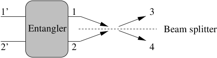
FIG. 1.: The setup for measuring the noise of entangled states. Uncorrelated electrons are fed into the entangler (see text) through the Fermi leads $1^{\prime}$, $2^{\prime}$ and are transformed into pairs of electrons in the entangled singlet (triplet) state $|\mp\rangle$, which are injected into leads $1$, $2$ (one electron of undetermined spin state into each lead). The entanglement of the, say, spin singlet can then be detected in an interference experiment using a beam splitter (with no backscattering): Since the orbital wave function of the singlet is symmetric, the electrons leave the scattering region preferably in the same lead ($3$ or $4$). This correlation (“bunching”) is revealed by an enhancement of the noise by a factor of $2$ in the outgoing leads.

Here the plus (minus) sign applies to spin-1/2 particles in the singlet (triplet) state, described by a (anti)symmetric orbital wave function. The very same two-particle interference mechanism which is responsible for the enhancement (reduction) of the scattering cross section $\sigma(\theta)$ near $\theta=\pi/2$ also leads to an increase (decrease) of the correlations of the particle number in the output arms of a beam splitter[16].

We turn now to the question of how to detect entanglement of electrons in a solid-state environment. For this we propose a non-equilibrium transport measurement using the set-up shown in Fig. 1. Here, the entangler is assumed to be a device by which entangled states of two electrons can be generated, a specific realization being above-mentioned double-dot system[10, 11]. The presence of a beam splitter ensures that the electrons leaving the entangler have a finite amplitude to be interchanged (without mutual interaction). Below we will show that in the absence of spin scattering the noise measured in the outgoing leads 3 and 4 will exhibit bunching behavior for pairs of electrons with a symmetric orbital wave function[17], i.e. for spin singlets, while antibunching behavior is found in the case of the spin triplets, due to their antisymmetric orbital wave function. The latter situation is the one considered so far for electrons in the normal state both in theory[18, 19] and in recent experiments[20, 21]. These experiments [20] have been performed in semiconducting nanostructures with geometries that are closely related to the set-up proposed in Fig. 1 but without entangler. Note that since the (maximally entangled) singlet is the only state leading to bunching behavior, the latter effect can be viewed as a unique signature for the entanglement of the injected electrons. To establish these results we first need to assess the effect of interactions in the leads. Thus we proceed in two steps: First, we show that the entanglement of electrons injected into Fermi leads is only partially degraded by electron-electron interactions. This allows us then to use, in a second step, the standard scattering matrix approach[18]—which we extend to a situation with entanglement—in terms of (non-interacting) Fermi liquid quasiparticles.

Entangled electrons in a Fermi liquid. Electrons are injected from the entangler (say, a pair of coupled quantum dots) into the leads, e.g. by (adiabatically) lowering the gate barriers between dot and lead, in the spin triplet (upper sign) or singlet (lower sign) state,

$$|\psi_{{\bf n}{\bf n^{\prime}}}^{t/s}\rangle={1\over\sqrt{2}}(a_{{\bf n}\uparrow}^{\dagger}a_{{\bf n^{\prime}}\downarrow}^{\dagger}\pm a_{{\bf n}\downarrow}^{\dagger}\,a_{{\bf n^{\prime}}\uparrow}^{\dagger}\,)\,|\psi_{0}\rangle,$$ (1)

with ${\bf n}=({\bf q},l)$, where ${\bf q}$ is the momentum of an electron, and $l$ is the lead number. Here, $\psi_{0}$ denotes the filled Fermi sea, the electronic ground state in the leads, and we have used the fermionic creation ($a^{\dagger}_{{\bf n}\sigma}$) and annihilation ($a_{{\bf n}\sigma}$) operators, where $\sigma$ denotes spin in the $\sigma_{z}$-basis. Next, we introduce the transition amplitude $G^{t/s}({\bf 1}{\bf 2},{\bf 3}{\bf 4};t)=\langle\psi^{t/s}_{{\bf 1}{\bf 2}},t|\psi^{t/s}_{{\bf 3}{\bf 4}}\rangle$ and define the fidelity as the modulus of $G^{t/s}$ between the same initial and final states, $|G^{t/s}({\bf 1}{\bf 2},{\bf 1}{\bf 2};t)|=|G^{t/s}({\bf 2}{\bf 1},{\bf 1}{\bf 2};t)|$. The fidelity is a measure of how much of the initial triplet (singlet) remains in the final state after propagating for time $t>0$ in a Fermi sea (metallic lead) of interacting electrons. We emphasize that after injection, the two electrons of interest are no longer distinguishable from the electrons of the leads, and consequently the two electrons taken out of the leads will, in general, not be the same as the ones injected. Introducing the notations $n=({\bf n},\sigma)$, and $\bar{n}=({\bf n},-\sigma)$, we write

$$G^{t/s}({\bf 1}{\bf 2},{\bf 3}{\bf 4};t)=-{1\over 2}\sum_{\sigma}\!\left[G(1\bar{2},3\bar{4};t)\pm G(1\bar{2},\bar{3}4;t)\right],$$ (2)

where we introduced the standard 2-particle Green’s function $G(12,34;t)=\langle\psi_{0}|Ta_{1}(t)a_{2}(t)a_{3}^{\dagger}a_{4}^{\dagger}|\psi_{0}\rangle$, with $T$ the time ordering operator. We assume a time- and spin-independent Hamiltonian, $H=H_{0}+\sum_{i<j}V_{ij}$, where $H_{0}$ describes the free motion of the $N$ electrons, and $V_{ij}$ is the bare Coulomb interaction between electrons $i$ and $j$.

The non-trivial many-body problem of finding an explicit value for $G(12,34;t)$ is simplified because we can assume that the leads $1$ and $2$ are sufficiently separated, so that the mutual Coulomb interaction can be safely neglected. This implies that the 2-particle vertex part vanishes and we obtain $G(12,34;t)=G(13,t)G(24,t)-G(14,t)G(23,t)$, i.e. the Hartree-Fock approximation is exact and the problem is reduced to the evaluation of single-particle Green’s functions $G({\bf n},t)=-i\langle\psi_{0}|Ta_{{\bf n}}(t)a_{{\bf n}}^{\dagger}|\psi_{0}\rangle\equiv G_{l}({\bf q},t)$, pertaining to lead $l=1,2$ (the leads are still interacting many-body systems though). Inserting this into Eq. (2) we arrive at the result $G^{t/s}({\bf 1}{\bf 2},{\bf 3}{\bf 4};t)=-G({\bf 1},t)\,G({\bf 2},t)[\delta_{{\bf 13}}\delta_{{\bf 24}}\mp\delta_{{\bf 14}}\delta_{{\bf 23}}]$, where the upper (lower) sign refers to the spin triplet (singlet). For the special case $t=0$, and no interactions, we have $G({\bf n},t)=-i$, and thus $G^{t/s}$ reduces to $\delta_{{\bf 13}}\delta_{{\bf 24}}\mp\delta_{{\bf 14}}\delta_{{\bf 23}}$, and the fidelity is $1$. In general, we have to evaluate the (time-ordered) single-particle Green’s functions $G_{1,2}$ close to the Fermi surface and obtain the standard result[22] $G_{1,2}({\bf q},t)\approx-iz_{q}\Theta(\epsilon_{q}-\epsilon_{F})e^{-i\epsilon_{q}t-\Gamma_{q}t}$, which is valid for $0\leq t\lesssim 1/\Gamma_{q}$, where $1/\Gamma_{q}$ is the quasiparticle lifetime, $\epsilon_{q}=q^{2}/2m$ the quasiparticle energy (of the added electron), and $\epsilon_{F}$ the Fermi energy. For a two-dimensional electron system (2DES), as e.g. in GaAs heterostructures, $\Gamma_{q}\propto(\epsilon_{q}-\epsilon_{F})^{2}\log(\epsilon_{q}-\epsilon_{F})$ [23] within the random phase approximation (RPA), which accounts for screening and which is obtained by summing all polarization diagrams[22]. Thus, the lifetime becomes infinite when the energy of the added electron approaches $\epsilon_{F}$ (with Fermi momentum $k_{F}$). The most important quantity in the present context is the renormalization factor or quasiparticle weight, $z_{F}=z_{k_{F}}$, evaluated at the Fermi surface, defined by $z_{F}=[1-\partial/\partial\omega\,{\rm Re}\Sigma(k_{F},\omega=0)]^{-1}$, where $\Sigma(q,\omega)$ is the irreducible self-energy. The quasiparticle weight, $0\leq z_{q}\leq 1$, describes the weight of the bare electron in the quasiparticle state ${\bf q}$. For momenta ${\bf q}$ close to the Fermi surface and for identical leads ($G_{1}=G_{2}$) we find

$$|G^{t/s}({\bf 1}{\bf 2},{\bf 3}{\bf 4};t)|=\,z_{F}^{2}\,|\,\delta_{{\bf 13}}\delta_{{\bf 24}}\mp\delta_{{\bf 14}}\delta_{{\bf 23}}|$$ (3)

for all times satisfying $0<t\lesssim 1/\Gamma_{q}$. Thus we find that the fidelity for singlet and triplet states in the presence of a Fermi sea and Coulomb interaction is given by $z_{F}^{2}$. Since this is the sought-for measure of the reduction of the spin correlation, it is interesting to evaluate $z_{F}$ explicitly for a 2DES. Evaluating $\Sigma$ within RPA (and imaginary time), we obtain ${\Sigma}({\bar{k}})=-(1/\Omega\beta)\sum_{\bar{q}}G^{0}({\bar{k}}+{\bar{q}})v_{q}\varepsilon({\bar{q}})$, where $\beta=1/k_{B}T$ is the inverse temperature, $\Omega$ the volume and ${\bar{q}}=(q_{n},{\bf q})$, with $q_{n}$ the Matsubara frequencies. The unperturbed Green’s function is given by $G^{0}({\bar{q}})=(iq_{n}-\xi_{\bf q})^{-1}$, where $\xi_{\bf q}=\varepsilon_{\bf q}-\varepsilon_{F}$, and the Coulomb interaction in two dimensions is $v_{q}=2\pi e^{2}/{q}$. The dielectric function can then be expressed as $\varepsilon=\varepsilon_{0}-v_{q}P^{(1)}({\bar{q}})$, using the polarization propagator in leading order, $P^{(1)}({\bar{q}})=-\Omega^{-1}\sum_{{\bf p},\sigma}[n_{F}(\xi_{\bf p})-n_{F}(\xi_{\bf p+q})]/[\xi_{\bf p}-\xi_{\bf p+q}+iq_{n}]$, where $n_{F}(\xi_{\bf p})=(e^{\beta\xi_{\bf p}}+1)^{-1}$. In two dimensions, we find $P^{(1)}({\bar{q}})=(2mk_{F}/\pi q){\rm Re}(\sqrt{u^{2}-1}-u)$, with $u={q}/2k_{F}+im\omega/{q}k_{F}$, and where the branch cut of $\sqrt{u^{2}-1}$ is on $[-1,1]$. After careful analytic continuation [22] and some lengthy calculation, we finally obtain

$$z_{F}=1-r_{s}\left({1\over 2}+{1\over\pi}\right),$$ (4)

in leading order of the interaction parameter $r_{s}=1/k_{F}a_{B}$, where $a_{B}=\epsilon_{0}\hbar^{2}/me^{2}$ is the Bohr radius. In particular, in a GaAs 2DES we have $a_{B}=10.3$ nm, and $r_{s}=0.614$, and thus we obtain $z_{F}=0.665$ [24, 25].

We see that the fidelity (spin correlation) is reduced by a factor of $z_{F}^{-2}\approx 2$ (from its maximum value $1$) as soon as we inject the two electrons (entangled or not) into separate leads consisting of interacting Fermi liquids in their ground state. Apart from this reduction, however, the entanglement is not affected by interacting electrons in the filled Fermi sea. This result allows us now to study the noise of entangled electrons using the standard scattering theory for quasiparticles in a Fermi liquid[26].

Noise of entangled electrons. We now investigate the noise correlations for scattering with the entangled incident state $|\pm\rangle\equiv|\psi_{{\bf 1}{\bf 2}}^{t/s}\rangle$, where we set ${\bf n}=(\varepsilon_{n},n)$, now using the electron energies $\varepsilon_{n}$ instead of the momentum as the orbital quantum number in Eq. (1) and where the operator $a^{\dagger}_{\alpha\sigma}(\varepsilon)$ creates an incoming electron in lead $\alpha$ with spin $\sigma$ and energy $\varepsilon$. (Another interesting spin effect is noise induced by spin transport[27].) First, we generalize the theory for the current correlations in a multiterminal conductor as given in Ref. [18] to the case of entangled scattering states, with the important consequence that Wick’s theorem cannot be applied directly. We start by writing the operator for the current carried by electrons in lead $\alpha$ of a multiterminal conductor as

$$I_{\alpha}(t)=\frac{e}{h\nu}\sum_{\varepsilon\varepsilon^{\prime}\sigma}\left[a_{\alpha\sigma}^{\dagger}(\varepsilon)a_{\alpha\sigma}(\varepsilon^{\prime})-b_{\alpha\sigma}^{\dagger}(\varepsilon)b_{\alpha\sigma}(\varepsilon^{\prime})\right]$$ (5)

$$\times\exp\left[i(\varepsilon-\varepsilon^{\prime})t/\hbar\right],$$ (6)

where the operators $b_{\alpha\sigma}(\varepsilon)$ for the outgoing electrons are related to the operators $a_{\alpha\sigma}(\varepsilon)$ for the incident electrons via $b_{\alpha\sigma}(\varepsilon)=\sum_{\beta}s_{\alpha\beta}a_{\beta\sigma}(\varepsilon)$, where $s_{\alpha\beta}$ denotes the scattering matrix. We assume that the scattering matrix is spin- and energy-independent. Note that since we are dealing with discrete energy states here, we normalize the operators $a_{\alpha\sigma}(\varepsilon)$ such that $\{a_{\alpha\sigma}(\varepsilon),a_{\beta\sigma^{\prime}}^{\dagger}(\varepsilon^{\prime})\}=\delta_{\sigma\sigma^{\prime}}\delta_{\alpha\beta}\delta_{\varepsilon\varepsilon^{\prime}}/\nu$, where the Kronecker symbol $\delta_{\varepsilon\varepsilon^{\prime}}$ equals $1$ if $\varepsilon=\varepsilon^{\prime}$ and $0$ otherwise. Therefore we also have to include the factor $1/\nu$ in the definition of the current, where $\nu$ stands for the density of states in the leads. We assume that each lead consists of only a single quantum channel; the generalization to leads with several channels is straightforward but is not needed here. Using the scattering matrix, we can write Eq. (6) as

$$I_{\alpha}(t)=\frac{e}{h\nu}\sum_{\varepsilon\varepsilon^{\prime}\sigma}\sum_{\beta\gamma}a_{\beta\sigma}^{\dagger}(\varepsilon)A_{\beta\gamma}^{\alpha}a_{\gamma\sigma}(\varepsilon^{\prime})e^{i(\varepsilon-\varepsilon^{\prime})t/\hbar},$$ (7)

$$A_{\beta\gamma}^{\alpha}=\delta_{\alpha\beta}\delta_{\alpha\gamma}-s_{\alpha\beta}^{*}s_{\alpha\gamma}.$$ (8)

The spectral density of the current fluctuations (noise) $\delta I_{\alpha}=I_{\alpha}-\langle I_{\alpha}\rangle$ between the leads $\alpha$ and $\beta$ is defined as

$$S_{\alpha\beta}({\omega})=\lim_{T\rightarrow\infty}\frac{h\nu}{T}\int_{0}^{T}\!\!\!dt\,\,e^{i\omega t}\,{\rm Re}\,\langle\pm|\delta I_{\alpha}(t)\delta I_{\beta}(0)|\pm\rangle.$$ (9)

We evaluate now the correlations Eq. (9) for zero frequency. Using the fact that the unpolarized currents are invariant when all spins are reversed, the expectation value $\langle\pm|\delta I_{\alpha}\delta I_{\beta}|\pm\rangle$ can be expressed as the sum of a direct and an exchange term, $\langle\pm|\delta I_{\alpha}\delta I_{\beta}|\pm\rangle=\langle\uparrow\downarrow\!|\delta I_{\alpha}\delta I_{\beta}|\!\uparrow\downarrow\rangle\pm\langle\uparrow\downarrow\!|\delta I_{\alpha}\delta I_{\beta}|\!\downarrow\uparrow\rangle$, where the upper (lower) sign of the exchange term refers to triplet (singlet). Evaluating these expressions further, we arrive at the following result for the zero-frequency ($\omega=0$) correlation between the leads $\alpha$ and $\beta$,

$$S_{\alpha\beta}\!=\!\frac{e^{2}}{h\nu}\Big{[}\sum_{\gamma\delta}\!{}^{{}^{\prime}}A_{\gamma\delta}^{\alpha}A_{\delta\gamma}^{\beta}\mp\delta_{\varepsilon_{1},\varepsilon_{2}}\big{(}A_{12}^{\alpha}A_{21}^{\beta}\!+\!A_{21}^{\alpha}A_{12}^{\beta}\big{)}\Big{]},$$ (10)

where $\sum_{\gamma\delta}^{\prime}$ denotes the sum over $\gamma=1,2$ and all $\delta\neq\gamma$, and where again the upper (lower) sign refers to triplets (singlets). The autocorrelations $S_{\alpha\alpha}$ determine the noise in lead $\alpha$ (note that $A_{\gamma\delta}^{\alpha}A_{\delta\gamma}^{\alpha}=|A_{\gamma\delta}^{\alpha}|^{2}$).

We apply our result Eq. (10) to the set-up shown in Fig. 1 involving four leads, described by the single-particle scattering matrix elements, $s_{31}=s_{42}=r$, and $s_{41}=s_{32}=t$, where $r$ and $t$ denote the reflection and transmission amplitudes at the beam splitter, respectively. We assume that there is no backscattering, $s_{12}=s_{34}=s_{\alpha\alpha}=0$. The unitarity of the s-matrix implies $|r|^{2}+|t|^{2}=1$, and ${\rm Re}[r^{*}t]=0$. Using Eqs. (8) and (10), we obtain the final result for the noise correlations for the incident state $|\pm\rangle$[29],

$$S_{33}=S_{44}=-S_{34}=2\frac{e^{2}}{h\nu}T\left(1-T\right)\left(1\mp\delta_{\varepsilon_{1}\varepsilon_{2}}\right),$$ (11)

where $T=|t|^{2}$ is the probability for transmission through the beam splitter. The calculation for the remaining two triplet states $|\!\uparrow\uparrow\rangle$ and $|\!\downarrow\downarrow\rangle$ yields the same result Eq. (11) (upper sign). For the average current in lead $\alpha$ we obtain $\left|\langle I_{\alpha}\rangle\right|=e/h\nu$, with no difference between singlets and triplets. Then, the Fano factor $F=S_{\alpha\alpha}/\left|\langle I_{\alpha}\rangle\right|$ takes the following form

$$F=2eT(1-T)\left(1\mp\delta_{\varepsilon_{1}\varepsilon_{2}}\right),$$ (12)

and correspondingly for the cross correlations. Eq. (12) is one of the main results of this work: it implies that if two electrons with the same energies, $\varepsilon_{1}=\varepsilon_{2}$, in the singlet state $|-\rangle$ are injected into the leads $1$ and $2$, then the zero frequency noise is enhanced by a factor of two, $F=4eT(1-T)$, compared to the shot noise of uncorrelated particles [18, 28], $F=2eT(1-T)$. This enhancement of noise is due to bunching of electrons in the outgoing leads, caused by the symmetric orbital wavefunction of the spin singlet $|-\rangle$. On the other hand, the triplet states $|+\rangle$ exhibit antibunching, i.e. a complete suppression of the noise, $S_{\alpha\alpha}=0$. The noise enhancement for the singlet $|-\rangle$ is a unique signature for entanglement (there exists no unentangled state with the same symmetry), therefore entanglement can be observed by measuring the noise power of a mesoscopic conductor as shown in Fig. 1. The triplets $|+\rangle$, $|\!\uparrow\uparrow\rangle$ and $|\!\downarrow\downarrow\rangle$ can be distinguished from each other by a measurement of the spins of the outgoing electrons, e.g. by inserting spin-selective tunneling devices[30] into leads $3$ and $4$.

In conclusion, we have demonstrated that entangled electrons (EPR pairs) can be transported in mesoscopic wires, and we have quantified the reduction of entanglement during this process. The current fluctuations in a beam-splitter set-up turn out to be a suitable experimental probe for detecting (entangled) spin states of electrons via their charge.

REFERENCES

- [1] A. Einstein, B. Podolsky, and N. Rosen, Phys. Rev. 47, 777 (1935).
- [2] C.H. Bennett, and G. Brassard, in Proceedings of the IEEE International Conference on Computers, Systems and Signal Processing, Bangalore, India (IEEE, New York, 1984), p. 175.
- [3] C.H. Bennett, and S.J. Wiesner, Phys. Rev. Lett. 69, 2881 (1992).
- [4] C.H. Bennett et al., Phys. Rev. Lett. 70, 1895 (1993).
- [5] J.S. Bell, Rev. Mod. Phys. 38, 447 (1966).
- [6] A. Aspect, J. Dalibard, and G. Roger, Phys. Rev. Lett. 49, 1804 (1982); W. Tittel et al., Phys. Rev. Lett. 81, 3563 (1998).
- [7] K. Mattle et al., Phys. Rev. Lett. 76, 4656 (1996).
- [8] D. Boumeester et al., Nature 390, 575 (1997); D. Boschi et al., Phys. Rev. Lett. 80, 1121 (1998).
- [9] J. M. Kikkawa et al., Science 277, 1284 (1997); J.A. Gupta et al., Phys. Rev. B59, R10421 (1999).
- [10] D. Loss and D.P. DiVincenzo, Phys. Rev. A 57, 120 (1998).
- [11] G. Burkard, D. Loss, and D. P. DiVincenzo, Phys. Rev. B 59 2070 (1999).
- [12] A. Imamoḡlu et al., Phys. Rev. Lett. 83, 4204 (1999).
- [13] C.H.W. Barnes, private communication.
- [14] R.P. Feynman, R.B. Leighton, M. Sands, The Feynman Lectures (Addison-Wesley, Reading, 1965), Vol. 3.
- [15] L.E. Ballentine, Quantum Mechanics, pp. 352, Prentice Hall, New Jersey, 1990.
- [16] R. Loudon, Phys. Rev. A 58, 4904 (1998).
- [17] R. Hanbury Brown and R. Q. Twiss, Nature (London) 177, 27 (1956).
- [18] M. Büttiker, Phys. Rev. Lett. 65, 2901 (1990); Phys. Rev. B46, 12485 (1992).
- [19] Th. Martin, R. Landauer, Phys. Rev. B45, 1742 (1992).
- [20] R.C. Liu et al., Nature 391, 263 (1998); M. Henny et al., Science 284, 296 (1999); W.D. Oliver et al., Science 284, 299 (1999).
- [21] For a positive sign in the noise cross correlations due to the boson-like properties of Cooper pairs see, J. Torrès and T. Martin, cond-mat/9906012.
- [22] G. D. Mahan, Many Particle Physics, 2nd Ed. (Plenum, New York, 1993).
- [23] G. F. Giuliani and J. J. Quinn, Phys. Rev. B 26, 4421 (1982).
- [24] After a more accurate numerical evaluation of the exact RPA self-energy, we find for GaAs .
- [25] For 3D metallic leads with say (e.g. ) the loss of correlation is somewhat less strong, since then the quasiparticle weight becomes , see T. M. Rice, Ann. Phys. 31, 100 (1965).
- [26] As in the unentangled case [18, 19, 28], we assume that the noise correlations that we find using the scattering-matrix approach are at most quantitatively but not qualitatively altered by Coulomb interactions.
- [27] Noise induced by spin currents can be observed in a two-terminal conductor attached to Fermi leads with spin-dependent bias . We have , and from Eq. (6) we obtain the noise power In particular, when we obtain the usual result[28] for the shot noise induced by the charge current . On the other hand, for , i.e. when there is no charge current through the conductor, , but still there is a non-vanishing spin current , one can observe the current noise induced by spin transport only.
- [28] V. A. Khlus, Zh. Eksp. Teor. Fiz. 93 2179 (1987) [Sov. Phys. JETP 66, 1243 (1987)]; R. Landauer, Physica D38, 226 (1989); G. B. Lesovik, Pis’ma Zh. Eksp. Teor. Fiz. 49, 513 (1989) [JETP Lett. 49, 592 (1989)].
- [29] For finite frequencies, we obtain the noise power . The noise contribution due to the Fermi sea is independent of the spin state of the injected pair.
- [30] G.A. Prinz, Science 282, 1660 (1998).