Measuring the Viscosity and Time Correlation Functions in a Microscopic Model of a Microemulsion

Abstract

A dynamical lattice model is used to study the viscosity and the velocity-velocity autocorrelation function in a microemulsion phase. We find evidence of anomalous viscosities in these phases (relative to water-rich and/or oil-rich phases), in qualitative agreement with other results. We also investigate the dynamic relaxation in the microemulsion phase. It has been suggested that the temporal relaxation in the microemulsion phase may be described by a stretched exponential Kolrausch-Williams-Watts law ($\phi(t)=A\exp[-(t/\tau)^{b}]$). In our model, we find the velocity-velocity autocorrelation function $\langle v(0)v(t)\rangle$ fits this law, showing both enhanced ($b>1$) and inhibited ($b<1$) diffusion.

]

I Introduction

Using models to study the microemulsion phase has been made difficult by the combination of short-ranged forces, short-range order, and long-ranged disorder exhibited. A large system is needed in order to observe the unique isotropic “structure”, while computer power dictates what is actually feasible. Very large systems can be handled by Monte Carlo (MC) simulations (either continuous or discretized), but the use of time-independent, non-physical moves prevents calculation of temporal observables. Molecular dynamics (MD) allows the measurement of interesting time-dependent properties, but also requires large numbers of independent particles. The upper capacity of MD is being continually stretched [1, 2, 3, 4, 5], but very large bulk systems are rarely effectively modeled.

There have been a number approaches have been used to balance these concerns [6, 7, 8, 9, 10, 11, 12]. In this paper, a dynamic lattice model introduced earlier [13] is further explored in which a Boltzmann velocity field is mapped onto a nearest-neighbor lattice model [14, 15], and the velocity field then is integrated into the metropolis MC scheme. It enables the determination of properties usually only accessible by Molecular Dynamics methods, and has been used to determine the diffusion constants and the dynamic surface tension between competing phases, with evidence of a corresponding wetting transition [16].

II Dynamic Monte Carlo

One of the aims in investigating complex surfactant systems is to generate a method which can be used to study both equilibrium and dynamic properties. Towards this goal, a general dynamic lattice MC model was constructed by combining Monte Carlo and Molecular Dynamic methods. This so called Dynamic Monte Carlo (DMC) simulation [13] takes advantage of both methods, and is able to be utilized in both equilibrium and nonequilibrium studies. This is used to investigate the dynamics of a lattice Monte Carlo, while keeping the equilibrium states of the model intact.

A Description of the DMC Model

The DMC simulation algorithm incorporates pseudo velocities into Monte Carlo calculations within a three-dimensional lattice model. In the base lattice model, cubic site $i$ is occupied by exactly one type of the three chemical species in a complex surfactant system. These are denoted by a statistical variable $\sigma_{i}$, which can take on the values $\{-1,0,+1\}$, corresponding to cubes of oil, surfactant, or water respectively. A vector variable $S_{i}$, defined at each lattice site, specifies the orientation of amphiphile particles. The water and oil sites give no orientation. This may be accomplished by the construction of a hybrid variable:

$$s_{i}=(1-\sigma^{2}_{i})S_{i}$$ (1)

Thus, only surfactant sites have a non-zero $s_{i}$. The variable $S_{i}$ is normalized as unit vector quantity that varies continuously in three dimensions.

The principle advantage of lattice models, compared to continuum models, is that they dramatically simplify the simulated motions of the particles. The particles may be located only at lattice sites, and there are no vacancies in the lattice. Therefore, each site cannot exchange with other sites independently. Only pairs of sites, together, can be considered for exchanges. This exchange is achieved by considering both the relative velocity between two nearest-neighbor sites, and the potential energy through the Metropolis algorithm. Although the simulation does not reflect realistic molecular sizes or individual molecular movement, the simplicity and short interaction range make the lattice model far easier to study in detail than continuum models, and the qualitative results obtained from the model well represent the macroscopic behavior of oil-water-surfactant systems.

In order to depict dynamics with this equilibrium model, a velocity field is applied to the lattice MC. The temperature of the simulation box fixes the kinetic energy of the particles in the system (a form of equipartition):

$$\frac{1}{2}\sum_{i=1}^{N}m_{i}v_{i}^{2}=\frac{3}{2}Nk_{B}T\quad.$$ (2)

At some time $t=0$ (really the first DMC step), the system is heated by randomly assigning velocities chosen from a Maxwell-Boltzmann distribution. The Maxwell distribution in one dimension is a special case of the Gauss(ian) normal distribution. Therefore, in each of the coordinate directions, the velocity components $v_{x}$, $v_{y}$, and $v_{z}$ obey the Gaussian distribution law. These velocities must be identified as an average or center-of-mass velocity of all the molecules within the lattice site, because of the multi-particle nature of each site. Thus, for a given temperature, we have

$$\left\langle m_{i}v_{\alpha\,i}^{2}\right\rangle=k_{B}T\quad,$$ (3)

where $\alpha$ is one of the three cartesian directions.

In the simulation, the movement of particles is achieved through the exchange of a pair of nearest-neighbors. As stated earlier, the energy of the system is independent of the orientation of the water and oil sites. Thus, including all desired features (treating water and oil sites as inversely symmetric, and treating the two ends of surfactant molecules symmetrically), the nearest-neighbor Hamiltonian may be written as

$${\cal H}=\frac{1}{2}{\sum_{\left\langle\mathbf{n},\mathbf{n^{\prime}}\right\rangle}}^{\prime}\bigg{[} c_{1}\sigma_{\mathbf{n}}(\Delta\mathbf{n}\cdot S_{\mathbf{n}^{\prime}})+c_{2}\sigma_{\mathbf{n}}^{2}(\Delta\mathbf{n}\cdot S_{\mathbf{n}^{\prime}})^{2}$$ (4)

$$+c_{3}\sigma_{\mathbf{n\phantom{{}^{\prime}}}}\sigma_{\mathbf{n}^{\prime}}+c_{4}\sigma_{\mathbf{n\phantom{{}^{\prime}}}}^{2}\sigma_{\mathbf{n}^{\prime}}^{2}\bigg{]}$$ (5)

$$+\sum_{\mathbf{n}}\big{[}\alpha\sigma_{\mathbf{n}}^{2}+\omega\sigma_{\mathbf{n}}\big{]}$$ (6)

where $\Delta\mathbf{n}\equiv\mathbf{n}-\mathbf{n}^{\prime}$ denotes the lattice difference vector between two sites $\mathbf{n}$ and $\mathbf{n}^{\prime}$; $\alpha$ and $\omega$ are the effective chemical potentials of water and oil; and the coupling constants $c_{\alpha}$ determine the bonding energies ($c_{1}=5/2$, $c_{2}=3/4$, $c_{3}=-3/8$, and $c_{4}=-1/6$). This creates a phase-diagram which includes a microemulsion phase. This nearest-neighbor sum runs over pairs of sites; each site has $2d$ neighbors in $d$ dimensions. By summing over all the particles in the system, the potential energy of the entire system is obtained.

At each simulation step, a pseudo-random walk is chosen through simulation space. A switch variable is used to choose one direction ($x$, $y$, or $z$), which ensures that each pair of nearest-neighbors are visited evenly. For each trial exchange, the change of total energy $\Delta E$ is obtained by evaluating both potential and kinetic energy differences. The potential energy factor is the difference of potential energy before and after the trial exchange. The kinetic energy is measured by the relative velocity $v=v_{\mathbf{n}}-v_{\mathbf{n}^{\prime}}$ only in the exchange direction. This means only the component of the velocity in the exchange direction is considered, and the components in the other two directions are unchanged through the trial exchange (and therefore any accepted exchange). The actual rules give results for the two possible signs of $v$: for the case $v<0$, no exchange occurs even for a favorable $\Delta E$, as a negative relative velocity corresponds to two particles moving away from each other. For $v>0$, a resulting (new) relative velocity $v^{\prime}$ is obtained:

$$\exp[-mv^{2}/2k_{B}T]=1-\exp[-m{v^{\prime}}^{2}/2k_{B}T]$$ (7)

In this manner, the final velocity components in the exchange direction are determined.

Both relative velocities and change of potential energy are considered for the change of total energy, and the acceptance or rejection of the exchange is then determined by the Metropolis algorithm. This implies that the kinetic energy can supply potential energy required exchange, or there can be mixing between the kinetic and potential energy. Since the velocities are initially assigned from a Maxwell-Boltzmann distribution, and retained throughout the trajectory, the potential energy should also be contained within a Boltzmann distribution of all the configurations obtained. For an accepted trial move, the chemical species within the two sites are exchanged, and the velocity components in the exchange direction will have new values resulting from Eq. (7); for a rejected trial move, an elastic collision is applied, so that the two particles move away from each other with an exchanged velocity component in the direction of collision.

The continuous spin variable $s_{\mathbf{n}}$ needs special treatment. Because surfactant molecules may move to neighbor sites, the orientation of newly created surfactant site must come from an equilibrated distribution to maintain detailed balance in the system. This is accomplished by creating a “ghost” vector orientation at each lattice site during the relaxation procedure. The ghost orientation at each site is also produced by Eq. (7), and acceptance comes by including the potential energy through the Metropolis algorithm. Therefore, the ghost orientations maintain equilibrium. When a surfactant moves to its neighbor site, it takes the ghost orientation of the site. System size is maintained by periodic boundary conditions.

B DMC Simulation in Practice

The microemulsion phase is studied by Dynamical Monte Carlo (DMC) simulation. Most simulations were performed on systems of $24\times 24\times 24$ lattice sites. A test of validity of the DMC method is examining the velocity distribution over time (DMC steps). The initial velocities of particles are generated according to a Maxwell-Boltzmann distribution. At the end of the simulation, velocities maintain the Maxwell-Boltzmann distribution as predicted. Additionally, there is the requirement that the DMC model maintains the equilibrium states from the standard MC. Results for the energies of systems of identical compositions from the two models, lattice MC and DMC, were indistinguishable.

Experiments indicate that the scattering intensity of microemulsion exhibits a peak at non-zero wavevector[17, 18, 19, 20, 21]. This scattering behavior is considered the signature of microemulsion, in contrast to normal disordered phases (which show an exponential decay with increasing wavevector). In the DMC, the scattering intensity is calculated as a discrete Fourier transformation of the water-water correlation function. We have chosen as a “typical” microemulsion system: 26% surfactant sites, 37% oil sites, and 37% water sites. An equilibrated microemulsion phase is obtained after 4000 to 6000 simulation full lattice passes (DMC steps). Simulated scattering data from such a phase is presented in Fig. 1.

FIG. 1.: Water-water structure function of microemulsion phase (T=1.5).

III Results and Discussion

A Viscosity of Microemulsion

The investigation of the viscosity of surfactant systems is of great interest for both scientific and industrial applications. Surfactant solutions show complicated rheological behavior. It has been shown experimentally that the viscosity of such systems is affected by many factors such as concentration, molecular volume, presence of electric charges, hydrodynamic interactions, and temperature. In practical terms, the viscosity of surfactant solutions is being scrutinized by industry. For example, the flow rate is strongly affected when these solutions are pumped through pipes or stirred in large containers. The viscosity is also relevant to the design of surfactant solution-based flooding processes, which can be utilized in oil recovery (following the primary and secondary stages). This is of great interest since some two-thirds of the oil originally in place can remain after the secondary recovery process.

The DMC has been used to investigate viscosity in microemulsion. A (unit) velocity gradient was applied to the system in one direction of the 3D lattice, in order to simulate the behavior of fluids under shear stress. The velocity component in $x$-direction ($v_{x}$) is forced to increase with increasing $y$. Across each lattice spacing, $v_{x}$ is increased by a constant amount (the shear rate) in the $y$-direction. The shear rate is a relative unit based on

$$\left\langle v_{\alpha}^{2}\right\rangle=1\quad(\alpha=x,y,z)\quad.$$ (8)

Since all the lattice sites on the same $xz$-plane suffer the same magnitude of shear, the exchanges between nearest-neighbors in the $xz$-plane are allowed to be performed normally. The exchange of particles across the $y$-direction, which exchanges between two adjacent $xz$-planes, needs to consider the different shear rates of the two lattice sites. The exchange of two particles by random motion may happen between sites in planes $y_{1}$ and $y_{2}$ (see Fig. 2).

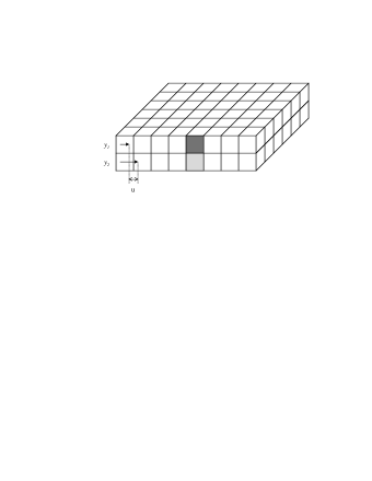
FIG. 2.: Schematic of the velocities of adjacent planes in the DMC.

Since the particle in $y_{1}$ has a lesser velocity component in the $x$-direction than does the particle in $y_{2}$, this exchange process involves a net transfer of momentum in the direction of $y$. For velocity components in the $y$- and $z$-direction ($v_{y}$ and $v_{z}$), the values are simply exchanged without any added effect. For the velocity component in the flow direction ($v_{x}$), the relative velocity is calculated as before, but the net transfer of momentum between the two planes is taken into account. The particle that moves from plane $y_{1}$ to $y_{2}$ is coming from a “slower” velocity field compared to particles in plane $y_{2}$. Therefore, its local velocity should be lower than its neighbors. On the other hand, the particle from plane $y_{2}$ should have a higher velocity than other particles in plane $y_{1}$. This can be summarized by the following expression for the final velocity component in the $x$-direction:

$$v_{x}(y_{1})=v_{x}(y_{2})+\mathbf{u}$$ (9a)

$$v_{x}(y_{2})=v_{x}(y_{1})-\mathbf{u}$$ (9b)

where $\mathbf{u}$ is the shear rate.

Viscosity has the generalized form[22]

$$\eta=\frac{N}{T}\frac{1}{2t}\left\langle(C_{v\mathbf{u}}(t))^{2}\right\rangle$$ (10)

which uses the velocity-velocity correlation function $C_{vv}(t)$. This can be re-written explicitly for $C_{vv}(t)$ with the result

$$2t\eta=\frac{N}{T}\left\langle\left(\sum_{i=1}^{N}\left[v_{ix}(t)\cdot\mathbf{u}-v_{ix}(0)\cdot\mathbf{u}\right]\right)^{2}\right\rangle$$ (11)

Use of the correlation function for viscosity measurements requires long lists of velocities for each particle at each DMC step. This large physical memory requirement is quite restrictive. Another way is to take advantage of the relative velocities used in the exchanges. Labeling this relative exchange velocity as $v_{ij,\alpha}$, we can use the sum

$$\eta=-\sum_{i,j}\frac{mv_{ij,x}-\mathbf{u}}{\mathbf{u}L^{3}\tau}$$ (12)

This sum is over only accepted exchanges of two nearest-neighbors in the $y$-direction. $L$ is the linear lattice size (generally, $L=24$ in this work). The variable $\tau$ is introduced as the reduced time step, which ensures that the average velocity is equal to the average rate of exchange of the sites ($\left\langle|v|\right\rangle\tau=\left\langle P(v)\right\rangle$). It is a constant of the simulation method. One of the advantages of this method is that it can work with periodic boundary conditions, since the shear rate of one site is only relative to its neighbors, and can only be considered during the exchange. Furthermore, since the flow is not explicitly introduced by increasing the velocity of each lattice site, and the kinetic energy is defined through local velocities (which are balanced during each exchange), any heating affect of the process is minimized.

Results for these viscosity measurements are presented in Table I. These results are for an equilibrated microemulsion phase (as determined by $S(k)$ data), at a constant temperature. The temperature can be independently determined through the kinetic energy. One can see that the apparent temperature falls as the shear rate is raised. This is due to the increased transference of kinetic energy to potential energy, also reflected in a corresponding increase in the potential energy.

TABLE I.: The viscosity from DMC of the microemulsion phase at $T=1.0$.

Shear Rate	Shear Viscosity ($\eta$)	Internal Energy	Final $T$
	$((\mathrm{m}J)^{1/3}/\ell)$	$(J)$	$(J/k_{\mathrm{B}})$
0.005	2.282	-1.448	0.979
0.010	1.862	-1.450	0.983
0.015	1.523	-1.461	0.983
0.020	1.371	-1.465	0.974
0.025	1.305	-1.469	0.969
0.030	1.227	-1.474	0.965

DMC calculations of the shear viscosity of microemulsion with shear rate changes exhibit some notable features, illustrated in Fig. 3.

FIG. 3.: The dependence of viscosity measurements on shear rate.

This bears some discussion about what is expected for such fluids. Currently, several studies of viscosity of microemulsion have been published in the literature. Gogarty and Dreher[23] have reported experimental results of microemulsion which shows strong non-Newtonian behavior. Many researchers have given values of microemulsion viscosity at only a single value of shear rate, or shear stress [24, 25, 26, 27, 28]. In some cases, non-Newtonian or anomalous behaviors were observed.[24, 25, 26, 28] However, there are several other researches which report Newtonian viscosities [29, 30, 31]. This may result from the contradictory elements of small interaction range and weak velocity variation. The hydrodynamic velocity gradients applied in these experiments are not high enough to create a strong velocity variation. Thus the system needs a relatively longer time to allow the velocity variation to be transferred compared to the renewal time of the system structure. This limitation is not always apparent in the microemulsion phase containing comparable amounts of water and oil. In particular, in a viscosity measurement of microemulsion obtained by a cone-and-plate rheometer, both Newtonian and non-Newtonian behaviors have been observed [32].

The data obtained from the DMC simulation exhibit a strong non-Newtonian behavior, which corresponds to only some of the experimental results. There is still much work to be done in this area before one can draw any conclusions as to which experimental results are correct (perhaps both sets are). However, we do know this behavior is not an artifact of the DMC, as water-rich (oil-rich) phases exhibit only Newtonian viscosities. On the other hand, there are some shear-induced perturbations in the simulation which may affect the viscosity results. The change of velocity component resulting from the shear is not an actual Boltzmann factor. This should affect the results of Metropolis algorithm in determining the acceptance or rejection of the exchange in the following simulation steps. In other words, a change of configuration is induced in the system corresponding to the shear rate. Evidence of this is the change of the internal energy and temperature of the system which are observed at high shear rate. Compared to the change of viscosity with shear rate, however, the affect of shear-induced error does not seem considerable. At lower shear rates, the results are seemly linear. In any case, in order to minimize the perturbation of shear on the system, and statistical error in calculation, the viscosity is determined at a relatively low shear rate. Thus, we shall now fix the shear rate at 0.01 (relative velocity units).

Purely thermal effects are also interesting to consider. Heuristically, viscosity should decrease with increasing temperature, but the overall behavior of microemulsion viscosity with temperature is not well understood. To investigate phase behavior of $\eta$, the shear viscosity of microemulsion phase was calculated and compared with the oil-rich phase at different temperatures. These results are presented in Table II and Figure 4.

TABLE II.: Shear viscosity of the microemulsion phase and the oil-rich phase ($\mathbf{u}=0.01$).

Temperature	$\eta$ (microemulsion)	$\eta$ (oil)
	($({\mathrm{m}}J)^{2}/\ell$)	($({\mathrm{m}}J)^{1/3}/\ell$)	% Change
1.0	1.862	1.979	5.9
1.2	1.764	1.920	8.1
1.5	1.761	1.850	4.8
1.7	1.738	1.812	4.1
2.0	1.689	1.764	4.2
2.2	1.652	1.736	4.8
2.5	1.650	1.699	2.9
2.7	1.627	1.678	3.0
3.0	1.619	1.648	1.8

FIG. 4.: The dependence of viscosity measurements on temperature.

One can see that with an increase in temperature, the viscosity of both phases decrease, which is characteristic of all liquids. At a given temperature, the microemulsion phase shows a considerably lower viscosity than the oil-rich phase, and this difference decreases with increasing temperature. Such behavior of microemulsion corresponds to the general experimental fact that the microemulsion phase exhibits low viscosity compared to other bulk phases.

It has been found experimentally that the viscosity of microemulsion is strongly affected by its microstructure. Papaioannou and coworkers[33] have published viscosity measurements of microemulsion as a function of salinity. They found that the viscosity of microemulsion exhibits two peaks: one at the oil-rich, and one at the water-rich phase boundaries. Additionally, a minimum was measured in the Winsor III state. It was also found through other experiments that the viscosity of microemulsion decreases as the structure becomes more and more bicontinuous.[34] In the DMC simulation, the microemulsion phase has comparable amounts of oil and water, corresponding to the bicontinuous Winsor III state. The DMC therefore shows good agreement with the experimental results.

B Long-time Behavior of the Velocity Auto-correlation Function

Use of the time-correlation function is one of the important approaches for describing transport processes and other time-dependent phenomena. This general function is considered to play a similar role in non-equilibrium Statistical Mechanics as the partition function plays in equilibrium situations. One advantage of the time-correlation function is that the resulting transport coefficients are quite general and independent of the details of any particular model. In particular, the self-diffusion coefficient can be expressed in terms of the velocity auto-correlation function as

$$D=\frac{1}{3}\int_{0}^{\infty}\left\langle v(0)\cdot v(t)\right\rangle\,\mathrm{d}t\quad.$$ (13)

This expression is valid for any classical system in which the diffusion is governed by the diffusion equation (Fick’s law). Therefore, the velocity auto-correlation function is a valuable approach to investigate the diffusion behavior of complex systems. Autocorrelation expressions like Eq. (13) may be nicely related to experiment. Observation of relaxation is a common experimental method to investigate the structure and dynamics of systems. Because both equilibrium and dynamical properties of the symmetric microemulsion phase are still very uncertain, the relaxation are of continuing importance.

The general form of velocity auto-correlation function is

$$C_{vv}(t)=\left\langle v(0)\cdot v(t)\right\rangle\quad.$$ (14)

When $t=0$, $C_{vv}(t)$ simply has the value of equilibrium average of $v^{2}(0)$ ($3k_{\mathrm{B}}T/m$ by equipartition). As time advances, $v(t)$ will be less correlated with its initial value. Thus, the velocity auto-correlation function is expected to decay to zero from its initial value. In general, it is assumed that any $C(t)$ decays exponentially with a time constant $\tau$. This can be expressed as

$$C(t)=A\exp\{-t/\tau\}\quad.$$ (15)

However, it has been found experimentally that time-relaxation in many disordered systems does not follow the simple exponential decay. The microemulsion phase is one example of this. Losada and López-Quintela [35] found a relaxation mode in microemulsion which follows a Kohlrausch-Williams-Watts (KWW) stretched-exponential law. The general form of this law is

$$\Phi(t)=A\exp\{-(t/\tau)^{b}\}\quad,\quad(0\leq b\leq 1)$$ (16)

The super-exponential factor $b$ was found to be dependent on many conditions, such as the spatial, temporal and energetic disorder of the system. There has been only limited discussion of the applicability of this law, and its ramifications [36, 37, 38].

In order to measure the velocity auto-correlation function in the DMC model, the derivative of the mean-squared displacement is used:

$$\frac{\partial\left\langle[r(t)-r(0)]^{2}\right\rangle}{\partial t}=\left\langle v(t)\cdot v(0)\right\rangle\quad.$$ (17)

In the DMC method, since the movement of particles is achieved only by the exchange of a pair of nearest-neighbors and is not explicitly decided by velocity of each single lattice site, a “measured” $\left\langle v(t)\cdot v(0)\right\rangle$ will not reflect the actual diffusive behavior of the system. The velocity auto-correlation function is therefore defined through Eq. (17).

Because of the average assembling nature of the velocity auto-correlation function, the long-time behavior is more difficult to observe and less accurate [39]. In determining whether relaxation follows a KWW-type law, the longest-time correlations are the most important. This requires extremely long simulation (cpu) times and proper equilibration before results may be examined. For a typical simulation, he velocity auto-correlation function is obtained from 3600 to 4000 equilibrated simulation lattice passes. Data obtained at different temperatures were fit to Eq. (16) for the longest part (last $2/3$) of simulation time — 1000 to 4000 DMC steps (Fig. 5). The fit is satisfactory for all microemulsion data obtained, and better than a simple exponential fit (Eq. (15)). Although all data (from $t=0$) were fit satisfactorially with either Eq. (15) or Eq. (16) (with $b\approx 1$), when only the longest-time data were included, the simple exponential fit was inadequate. Thus, Eq. (16) fits the entire data range well, while Eq. (15) breaks down at longer “times”. Additionally, auto-correlation data obtained from the DMC in the water-rich or oil-rich phases can not be found to fit a “pure” ($b\neq 1$) KWW law. The values of the KWW fit parameters are presented in Table III.

FIG. 5.: KWW stretched-exponential law fit to data of velocity auto-correlation function of microemulsion phase (T=1.5).

TABLE III.: Temperature dependence of the KWW equation parameters in the microemulsion phase (A=0.1).

Temperature	$\tau$	$b$
2.5	145.63	1.365
2.2	121.67	1.054
2.0	105.79	0.840
1.7	82.48	0.630
1.5	69.67	0.575
1.3	58.55	0.490
1.2	53.65	0.470
1.1	50.48	0.459
1.0	48.71	0.418

Both the stretched exponent $b$ and the macroscopic relaxation time $\tau$ are found to increase with increasing temperature within the microemulsion phase. The increase in relaxation time may be understood as a slowing of the diffusion rate as the system approaches the critical temperature. A number of reports have been published on the experimental study of critical phenomena of surfactant systems [34]. However, the critical behavior in surfactant solutions is still far from being understood completely. One common feature found in most of the investigations is that phase separation occurs as temperature is raised. This may be related to the slowing of diffusive behavior, observed in the present model.

The wide variation of $b$ is of great interest. Notably, a value of $b$ greater than 1 was obtained at high temperatures, which has not been observed in normal disordered phases. This corresponds to “enhanced diffusion” — faster than expected. Losada [35] has reported a relaxation study of microemulsion using a pressure-jump technique. In this experiment, the relaxation behavior with $b>1$ was observed in a microemulsion phase that had similar concentrations of oil and water. This has been the only experimentally-observed example of enhanced diffusion in microemulsion. It is hoped that additional work in this area will be done to confirm this interesting and important result.

The stretched exponent $b$ is strongly temperature-dependent. It has been treated by the theory of critical phenomena, and Losada found that it fit the critical equation

$$b=A\,[(T_{c}-T)/T_{c}]^{-1}$$ (18)

The temperature dependence of $b$ was measured by DMC simulation in order to confirm this behavior. The DMC data was fit to Eq. 18 (Fig. 6). This fit resulted in the value $A=0.30$, and gave a critical temperature $T_{c}=3.20$. From Fig 6 one can see that $b=1$ when $T=2.21$; at this point, the relaxation (as well as the diffusion) is “normal” and the KWW equation reduces to the exponential form. At temperatures below this point, the microemulsion shows an inhibited diffusive behavior. This can be related to the spatial and temporal disorder present in the system. It has been found in both experimental and theoretical research that diffusion behavior moves from anomalous to normal as the temperature is increased[40, 41]. This corresponds to DMC results obtained for $T<2.21$. As the temperature is increased past this point, there is an enhancement of diffusion in the system.

FIG. 6.: Temperature dependence of the stretched exponent $b$.

IV Conclusions

The complex systems formed between oil, water and surfactant molecules were examined with a three-dimensional lattice model enhanced by the addition of a coarse-grained velocity field. The shear viscosity of microemulsion phase was measured as a function of shear rate, and showed a decrease as the shear rate increased. The measurements were also performed on oil-rich phases, which showed typical behavior of a Newtonian (classical) fluid. Compared to the oil-rich phase, the viscosity of microemulsion shows strong non-Newtonian behavior. This corresponds to at least one experimental observation of the existence of non-Newtonian shear behavior in microemulsion [32, 28] The shear viscosities were also measured as a function of temperature. In all the systems simulated here, the microemulsion phase shows a notably lower viscosity than the oil-rich phase. As the temperature approaches to the critical temperature, the difference decreases. We would expect the two viscosities to equal at the thermodynamic limit. These viscosity measurements in the microemulsion phase qualitatively reproduce experimental observations [33, 34].

Measurements of the velocity autocorrelation function were obtained by the distance displacement method. The most interesting observation is that the long-time tails of microemulsion do not obey a simple exponential decay, but rather a Kohlrausch-Williams-Watts stretched-exponential law. The same behavior has been observed experimentally in a few other disordered phases [35, 42]. Microemulsion, a particular disordered phase, shows many properties distinct from normal disordered phases, which makes the long-time behavior very compelling. Both the stretched exponent and the macroscopic relaxation time were found to be strongly temperature-dependent. The temperature dependence of the super-exponential $b$, shows critical scaling. The values of $b$ can be divided into three temporal ranges $b=1,b<1,b>1$. Since the velocity autocorrelation function is directly related to the diffusion constant, this suggests the existence of normal, inhibited and enhanced diffusion in this model. These results provide evidence that DMC method employed in this work should be capable of simulate not only the equilibrium but the dynamics of the system as well. The diffusion constants and the dynamic surface tension between microemulsion and oil-rich phases has already been calculated [16], and the measurement of other properties should also be possible through use of the DMC model.

Due to the fact that the molecules are defined at the lattice sites, the movements of particles are restricted to unit length. Consequently, the velocities involved in the calculations are not completely realistic. In particular, a small spatial region of the velocity autocorrelation function is anti-correlated and inaccurate at certain degree. Furthermore, we make no attempt to make quantitative comparisons of shear viscosity with experimental data. Such comparison would require more realistic modeling of the molecular interactions.

One aspect of future work may connect velocity autocorrelation function results to the cooperative relaxation behavior of the system. The dipole correlation function is one way to describe of the mechanism of cooperative relaxation through experiment, so that the velocity autocorrelation function can be related to the relaxation of the dipole moment in droplets, as well as the structural and kinetic properties of the system. The observed non-Newtonian behavior is a macroscopic representation of the microstructure of microemulsion. However, at present there is little theory to connect these viscosity observations with microstructural evolution. Since both Newtonian and non-Newtonian regimes have been observed experimentally, this phase progression of microemulsion is of interest to explore further.

REFERENCES

- [1] J. Bocker, J. Brickmann, and P. Bopp, J. Phys. Chem. 98, 712 (1994).
- [2] M. J. Neuvo, J. Morales, and D. M. Heyes, Phys. Rev. E 58, 5845 (1998).
- [3] M. Tarek, S. Bandyopadhyay, and M. L. Klein, J. Mol. Liquids 78, 1 (1998).
- [4] N. M. Van Os, L. A. M. Rupert, B. Smit, P. A. J. Hilbers, K. Esselink, M. R. Bohmer, L. K. Koopal, Coll. Surf. A 81, 217 (1993).
- [5] B. Smit, P. A. J. Hilbers, K. Esselink, L. A. M. Rupert, N. M. van Os, and A. G. Schlijper, Nature 348, 624 (1990).
- [6] O. Theissen, G. Gompper, and D. M. Kroll, Europhys. Lett. 42, 419 (1998).
- [7] S. M. Willemsen, T. J. H. Vlugt, C. J. Hoefsloot, and B. Smit, J. Comp. Phys. 147, 507 (1998).
- [8] J. S. Sá Martins and P. M. C. de Oliveira, Nuc. Phys. A 643, 433 (1998).
- [9] T. D. Blake, J. De Coninck, and U. D’Ortona, Langmuir 11, 4588 (1995).
- [10] H. Stassen and W. A. Steele, J. Chem. Phys. 102, 932 (1995).
- [11] M. Gerits, M. H. Ernst, and D. Frenkel, Phys. Rev. E 48, 988 (1992).
- [12] A. N. Emerton, P. V. Coveney, and B. M. Boghosian, Physica A 239, 373 (1997); B. M. Boghosian, F. J. Alexander, and P. V. Coveney, Int. J. Mod. Phys. C 8, 637 (1997); B. M. Boghosian, P. V. Coveney, and A. N. Emerton, Proc. Roy. Soc. Lon. A, 452, 1221 (1996).
- [13] J. R. Gunn, C. M. McCallum, and K. A. Dawson, Phys. Rev. E 47, 3069 (1993).
- [14] K. A. Dawson and Zoran Kurtović J. Chem. Phys 92, 5473, (1990).
- [15] J. R. Gunn and K. A. Dawson, J. Chem. Phys. 96, 3152 (1992).
- [16] C. M. McCallum and J. R. Gunn, unpublished.
- [17] V. Degiorgio and M. Corti, Chem. Phys. Lett. 151, 349 (1988).
- [18] S. H. Chen, S. L. Chang, and R. Strey, J. Chem. Phys. 93, 1907 (1990).
- [19] S. Berr, R. R. M. Jones, J. S. Johnson, J. Phys. Chem. 96, 5611 (1992).
- [20] G. Gompper and M. Hennes, Phys. Rev. Lett. 73, 1114 (1994).
- [21] F. Mallamace, N. Micali, and S. H. Chen, Physica A 235, 170 (1997).
- [22] D. F. Eggers, N. W. Gregory, G. D. Halsey and B. S. Rabinovitch, Physical Chemistry. (John Wiley & Sons, Inc., New York 1964).
- [23] K. D. Dreher, W. B. Gogarty and R. D. Syndansk, J. Colloid Interface Sci. 57, 379 (1976).
- [24] D. Attwood, L. R. J. Currie, and P. H. Elworthy, J. Colloid Interface Sci. 46, 379 (1974).
- [25] R. N. Healy and R. L. Reed, Soc. Pet. Eng. J. 14, 491 (1974).
- [26] R. N. Healy, R. L. Reed and D. G. Stenmark, Soc. Pet. Eng. J. 16, 147 (1976).
- [27] S. C. Jones and K. D. Dreher, Soc. Pet. Eng.J. 16, 161 (1976).
- [28] E. Acosta, D. H. Kurlat, M. Bisceglia, B. Ginzberg, L. Baikauskas, and S. D. Romano, Coll. Surf. A 106, 11 (1998).
- [29] M. Dvolaitzky, M. Guyot, M. Lagues, J. P. Lepesant, R. Ober, C. Sauterey, and C. Taupin, J. Chem. Phys. 69, 3279 (1978).
- [30] G. B. Thurston, J. L. Salager, and R. S. Schechter, J. Colloid Interface Sci. 70, 517 (1979).
- [31] A. M. Bellocq, J. Biais, B. Clin, P. Lalanne, and B. Lemanceau, J. Colloid Interface Sci. 70, 524 (1979).
- [32] B. M. Knickerbocker, C. V. Pesheck, L. E. Scriven, and H. T. Davis, J. Chem. Phys. 83, 1984 (1979).
- [33] K. L. Mittal and P. Bothorel, Surfactants in Solution, Vol. 6, (Plenum, New York 1986).
- [34] K. L. Mittal, Surfactants in Solution, Vol. 10, (Plenum, New York 1989).
- [35] M. A. López-Quintela and D. Losada, Phys. Rev. Lett. 61, 1131 (1988).
- [36] M. A. López-Quintela, C. Tojo, and M. C. Bujannunuez, Mol. Phys. 74, 785 (1991).
- [37] G. H. Weiss, M. Dishon, A. M. Long, J. T. Bendler, A. A. Jones, P. T. Inglefield, and A. Bandis, Polymer 35, 1880 (1994).
- [38] M. A. Vanderhoef and D. Frenkel, Phys. Rev. A 41, 4277 (1990).
- [39] J. E. Variyar and D. Kivelson, J. Chem. Phys. 97, 8549 (1992).
- [40] W. P. Keirstead and B. A. Huberman, Phys. Rev. A 36, 5392 (1987).
- [41] J. Kakalios, R. A. Street, and W. B. Jackson, Phys. Rev. Lett. 59, 1037 (1987).
- [42] M. Daoud and J. Klafter, J. Phys. A: Math. Gen. 23, L981 (1990).