Boundary critical behaviour of two-dimensional random Potts models

Abstract

We consider random $q$-state Potts models for $3\leq q\leq 8$ on the square lattice where the ferromagnetic couplings take two values $J_{1}>J_{2}$ with equal probabilities. For any $q$ the model exhibits a continuous phase transition both in the bulk and at the boundary. Using Monte Carlo techniques the surface and the bulk magnetizations are studied close to the critical temperature and the critical exponents $\beta_{1}$ and $\beta$ are determined. In the strip-like geometry the critical magnetization profile is investigated with free-fixed spin boundary condition and the characteristic scaling dimension, $\beta_{1}/\nu$, is calculated from conformal field theory. The critical exponents and scaling dimensions are found monotonously increasing with $q$. Anomalous dimensions of the relevant scaling fields are estimated and the multifractal behaviour at criticality is also analyzed.

1 Introduction

The presence of quenched i.e. time independent disorder could modify the cooperative behaviour of physical systems with many degrees of freedom. In classical systems, where thermal fluctuations dominate quantum fluctuations the effect of disorder in the pure system phase-transition point can be analyzed by relevance-irrelevance criterions. For second-order transitions, according to the well known Harris criterion harris74 , disorder appears to be a relevant perturbation which moves the random system towards a new fixed point when the specific heat exponent $\alpha$ of the pure system is positive. In the other situation, $\alpha<0$, the disordered system remains in the pure model universality class. The two-dimensional random-bond Ising model (RBIM) corresponds to the marginal case. It has been extensively studied in the 80’s (for reviews of theoretical and numerical studies, see Refs. shalaev94 and selkeshchurtalapov94 , respectively). The effect of randomness on first-order phase transitions was considered later. Imry and Wortis argued that quenched disorder could induce a second-order phase transition imrywortis79 . This argument was then rigorously proved by Aizenman and Wehr, and Hui and Berker aizenmanwehr89 ; huiberker89 : In two dimensions, even an infinitesimal amount of quenched impurities changes the transition into a continuous one.

The random bond Potts model (RBPM) is the paradigm of systems the pure version of which undergoes a second-order or a first-order transition, depending on the number of states, $q$, per spin wu82 . In two dimensions, the second-order regime $q\leq 4$ has been considered by a number of authors, using perturbative field-theoretical techniques ludwig87 ; ludwigcardy87 ; ludwig90 ; dotsenkopiccopujol95a ; jugshalaev ; dotsenko95 or Monte Carlo (MC) simulations wisemandomany95 ; picco96 ; kim96 . On the other hand, in the first-order regime, $q>4$, conformal perturbation techniques can not be used around the pure model transition point and the resort to numerical calculations becomes essential. Both Monte Carlo simulations and Transfer Matrix (TM) techniques, combined to standard Finite Size Scaling (FSS) chenferrenberglandau92 ; chenferrenberglandau95 ; chatelainberche98 ; yasar98 ; picco98 ; olsonyoung99 and conformal methods picco97 ; cardyjacobsen97 ; jacobsencardy98 ; chatelainberche98b ; chatelainberche99 were used at the random fixed point of self-dual disordered models to study bulk critical properties.

The surface properties of dilute or random-bond magnetic systems were on the other hand paid less attention. Generally surface quantities, such as magnetization, energy-density, etc. are characterized by a different set of scaling dimensions, than their bulk counterparts. For example in the pure Ising model, bulk magnetization vanishes as $m\sim t^{\beta}$, with $\beta=1/8$, whereas for the surface magnetization the decay-law, $m_{1}\sim t^{\beta_{1}}$, involves the surface exponent $\beta_{1}=1/2$, where $t$ denotes the reduced temperature. Quite generally, the scaling laws involving surface and/or bulk exponents can be deduced from the assumption of scale invariance. For example the singular part of the bulk, $f_{\rm b}$, and surface, $f_{\rm s}$, free-energy densities in a $d$-dimensional system behave under a scaling transformation, when lengths are rescaled by a factor $b>1$, $l^{\prime}=l/b$, as

$$f_{\rm b}(t,h)=b^{-d}f_{\rm b}(b^{y_{t}}t,b^{y_{h}}h),$$ (1)

$$f_{\rm s}(t,h,h_{s})=b^{-(d-1)}f_{\rm s}(b^{y_{t}}t,b^{y_{h}}h,b^{y_{h_{s}}}h_{s}).$$ (2)

The whole set of bulk and surface critical exponents can be expressed in terms of the anomalous dimensions $y_{i}$ associated to the relevant scaling fields binder83 (temperature $t$, bulk $h$ and boundary $h_{s}$ magnetic fields), for example $\beta=(d-y_{h})/y_{t}$ and $\beta_{1}=(d-1-y_{h_{s}})/y_{t}$.

The $(1,1)$ surface of the disordered Ising model on a square lattice has recently been investigated through MC simulations by Selke et al. selkeetal97 ; igloietal98 . (For a related study of the critical behaviour at an internal defect line in the disordered Ising model, see Ref. szalmaigloi99 .) The critical exponent $\beta_{1}$ was found robust against dilution keeping the pure system value $\beta_{1}=1/2$ and no logarithmic correction has been observed, in contradistinction with the corresponding bulk behaviour. The surface properties of the 8-state RBPM were also considered in Refs. chatelainberche98 ; chatelainberche99 .

In this paper, we report extensive MC and Transfer Matrix studies of the critical behaviour of both the surface and bulk magnetizations of the disordered Potts ferromagnets for different values of $3\leq q\leq 8$. Our study extends previous investigations in several directions. First, we investigate the temperature dependence of the bulk and surface magnetizations and calculate the critical exponents $\beta$ and $\beta_{1}$. Second, we consider strip-like systems with fixed spin boundary conditions (BC), determine the magnetization profile at the critical temperature and calculate the scaling dimensions $x_{b}=2-y_{h}=\beta/\nu$ and $x_{1}=1-y_{h_{s}}=\beta_{1}/\nu$ from predictions of conformal invariance. Our third investigation concerns the possible multifractal behaviour of the correlation function and the critical magnetization profile. The $n$-th moments of both quantities are found to follow predictions of conformal invariance and the scaling dimensions $x_{b}^{(n)}$ and $x_{1}^{(n)}$ are obtained $n$-dependent.

The structure of the paper is the following. In Section 2, we present briefly the model and the simulation techniques. Section 3 is devoted to the approach to criticality, while in Section 4, magnetization profiles in the transverse direction of strips with fixed-free boundary conditions are computed. Multifractality is studied in Section 5 and a discussion of the results is given in Section 6.

2 Model and algorithms

2.1 The random-bond Potts model

We consider Potts-spin variables, $\sigma_{l,k}\in{1,2,\dots,q}$ on the sites of a square lattice with $l=1,2,\dots,L$ columns and $k=1,2,\dots,K$ rows, with independent random nearest-neighbour ferromagnetic interactions $J_{lk}$ and $J^{\prime}_{lk}$ in the horizontal and vertical directions, respectively, which have the same distribution and could take two values, $J_{1}>J_{2}$, with equal probabilities:

$${\cal P}(J_{lk})=\frac{1}{2}\delta(J_{lk}-J_{1})+\frac{1}{2}\delta(J_{lk}-J_{2}).$$ (3)

The Hamiltonian of the model is thus written

$$-{\cal H}=\sum_{l,k}\left(J_{lk}\delta_{\sigma_{l,k},\sigma_{l+1,k}}+J^{\prime}_{lk}\delta_{\sigma_{l,k},\sigma_{l,k+1}}\right).$$ (4)

In the thermodynamic limit $L,K\to\infty$ the model is self-dual and the self-duality point

$$[\exp(J_{1}/k_{B}T_{c})-1][\exp(J_{2}/k_{B}T_{c})-1]=q\;,$$ (5)

corresponds to the critical point of the model if only one phase transition takes place in the system. This assumption is strongly supported by numerical calculations.

The degree of dilution in the system can be varied by changing the ratio of the strong and weak couplings, $r=J_{1}/J_{2}$. At $r=1$, one recovers the perfect $q$-state Potts model, whereas for $r\to\infty$ we are in the percolation limit, where $T_{c}=0$. The intermediate regime of dilution $1<r<\infty$ is expected to be controlled by the random fixed-point located at some $r=r^{\star}(q)$.

2.2 Monte Carlo simulations

For the simulation of spin systems, standard Metropolis algorithms based on local updates of single spins suffer from the well known critical slowing down. As the second-order phase transition is approached, the correlation length becomes longer and the system contains larger and larger clusters in which all the spins are in the same state. Statistically independent configurations can be obtained by local iteration rules only after a long dynamical evolution which needs a huge number of MC steps and makes this type of algorithm inefficient close to a critical point.

Since disorder changes the transition of the Potts model into a second-order one, the resort to cluster update algorithms is more convenient janke96 ; barkemanewmann97 . These algorithms are based on the Fortuin-Kasteleyn representation fortuinkasteleyn69 where bond variables are introduced. In the Swendsen-Wang algorithm swendsenwang87 , a cluster update sweep consists of three steps: Depending on the nearest neighbour exchange interactions, assign values to the bond variables, then identify clusters of spins connected by active bonds, and eventually assign a random value to all the spins in a given cluster. The Wolff algorithm wolff89 is a simpler variant in which only a single cluster is flipped at a time. A spin is randomly chosen, then the cluster connected with this spin is constructed and all the spins in the cluster are updated.

Both algorithms considerably improve the efficiency close to the critical point and their performances are comparable in two dimensions, so in principle one can equally choose either one of them. Nevertheless, when one uses particular boundary conditions, with fixed spins along some surface for example, the Wolff algorithm is less efficient, since close to criticality the unique cluster will often reach the boundary and no update is made in this case. In the following, we will consider two different series of simulations, one with free BC where the Wolff algorithm will be used, and the other with fixed-free BC for which we have chosen the Swendsen-Wang algorithm.

3 Approach to criticality

In this Section we consider square shaped systems, where $L$ and $K$ are equal, with $L$ ranging from $40$ to $640$ to check finite size effects. In the vertical direction we impose periodic boundary conditions, thus $\sigma_{l,K+1}\equiv\sigma_{l,1}$, for $l=1,2,\dots,L$, whereas in the horizontal direction the boundary spins at $l=1$ and $l=L$ are free. Thus we have a pair of $(0,1)$ surfaces, obtained by cutting bonds along the vertical axis of the system.

According to numerical studies about the bulk quantities of the random model the finite size corrections are very strong unless the calculations are performed close to the random fixed-point chatelainberche99 . The approximate position of $r^{*}(q)$ is listed in Table 3 for different values of $q$, as obtained from the maximum condition of the central charge of the model chatelainberche99 ; dotsenkojacobsenlewispicco98 . Our simulations were performed at these fixed-point values of the dilution, but for comparison we have also considered systems with somewhat different values of $r$.

We averaged over an ensemble of bond configurations and the number of different realizations ranged from several hundreds to several thousands. In the simulations the one-cluster flip Monte Carlo algorithm was used, generating several $10^{4}$ clusters per realization close to the critical point. As in earlier studies the statistical errors for each realization were significantly smaller than those obtained by averaging over the different realizations. This is the reason of using a relatively large number of realizations in the ensemble averaging. The details of the parameters used in the MC simulations are given in the case $q=8$, $r=10$ in Table 1.

Table 1: Details of the parameters used for MC computations (Wolff algorithm). These values are given for the case $q=8$, $r=10$. 25% of cluster flips have been discarded for thermalization.

$t$	$L\times K$	# of realizations	# of cluster flips
0.02	640$\times$320	317	10000
0.05	160$\times$160	150	10000
	320$\times$320	184	10000
	640$\times$320	291	10000
0.1	320$\times$320	303	10000
0.15	320$\times$320	303	10000
	160$\times$320	84	10000
	160$\times$160	56	10000
0.175	160$\times$160	100	10000
0.2	320$\times$320	119	10000
0.225	160$\times$160	100	5000
0.25	160$\times$160	187	5000
0.275	160$\times$160	100	5000
0.3	160$\times$160	187	5000
	80$\times$160	400	5000
0.35	160$\times$160	187	5000
0.4	160$\times$160	187	5000
0.45	160$\times$160	187	5000
0.5	160$\times$160	187	5000

In the MC simulations we calculated the magnetization profile, defined as

$$[m(l)]_{\rm av}={1\over K}[|\sum_{k}m_{l,k}|]_{\rm av}\;,$$ (6)

where $m_{l,k}=(q\langle\delta_{\sigma_{l,k},1}\rangle-1)/(q-1)$ is the local Potts order-parameter and the summation goes over the spins in the $l$-th column, $k=1,2,\dots,K$. The brackets $\langle\dots\rangle$ and $[\dots]_{\rm av}$ stand for thermal and ensemble averages, respectively. The absolute values are taken in order to obtain non-vanishing profiles for finite systems. The surface magnetization is given by $[m_{1}]_{\rm av}=[m(1)]_{\rm av}=[m(L)]_{\rm av}$.

Figure 1: Profile of the $q=6$ model with free BC for two values of $r$ at a distance $t=0.02$ from the critical point. The size is $320\times 320$ and average was performed over 180 and 44 realizations of disorder for $r=8$ and 10, respectively.

The local magnetization, $[m(l)]_{\rm av}$, shows a monotonic decrease on approach to the free surface, due to the reduced coordination number close to the boundary. This is illustrated in Figure 1 for the random $q=6$ model with dilutions $r=8$ and $r=10$ at the same distance $t=0.02$ from the critical temperature $T_{c}$ in equation (5). The reduced temperature is defined by $t=\mid K-K_{c}\mid/K$ where $K=J/k_{B}T$. As it can be seen, the randomness tends to reduce order, thus the magnetization is decreasing with dilution. The magnetization profile displays a plateau at the center of the system, the value of which defines the bulk magnetization, $[m_{b}]_{\rm av}=[m(L/2)]_{\rm av}$, at the given temperature. The surface region of the profile has a characteristic size of $\xi_{r}$, which is expected to scale like to the bulk correlation length, $\xi\sim t^{-\nu}$, as the critical point is approached. For the random Potts model the correlation length exponent, $\nu$, is close to $1$, for all values of $q$ cardyjacobsen97 .

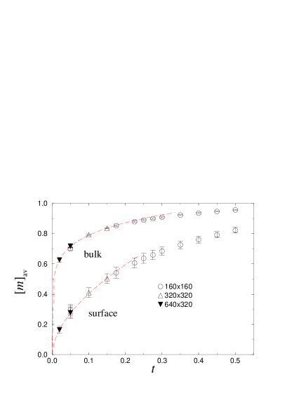
Figure 2: Temperature dependence of the surface and bulk magnetization ($q=8$, $r=10$). The dashed lines are guide for the eyes where the extrapolated exponents of Table 3 have been used.

In the thermodynamic limit, $L\to\infty$, as the critical temperature $T_{c}$ in (5) is approached, the magnetization profile $[m(l)]_{\rm av}$ goes to zero as a power-law, $[m(l)]_{\rm av}\sim t^{\beta(l)}$, where $\beta(1)=\beta(L)=\beta_{1}$ and $\beta(l)=\beta$ for $\xi_{r}<l<L-\xi_{r}$, where $\beta_{1}$ and $\beta$ are the usual surface and bulk critical exponents, respectively. The temperature dependence of bulk and surface magnetization is shown in Figure 2. To estimate the values of these critical exponents from simulation data one may define temperature-dependent effective exponents

$$\beta_{\rm eff}(l)=\frac{{\rm d}\ln[m(l)]_{\rm av}}{{\rm d}\ln t}\;,$$ (7)

which are approximated by using data at discrete temperatures, say, $t+\Delta t/2$ and $t-\Delta t/2$. In the limit of sufficiently small $\Delta t$ and $t$ the effective exponents approach the true critical exponents, presuming that the system is large enough so that finite-size effects play no role (to avoid finite-size effects, $L$ should be much larger than the size of the surface region, $\xi_{r}$, and the bulk correlation length, $\xi$).

Figure 3: Temperature-dependent effective exponents $\beta_{\rm eff}(l)$ for the surface and bulk magnetization for $q=8$, $r=10$. In the case of the bulk, the error bars are smaller than the symbol sizes.

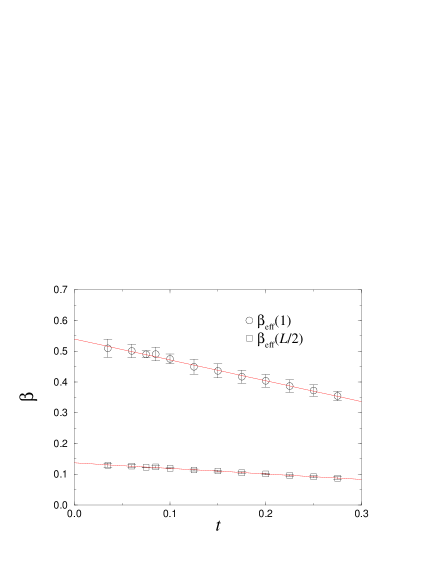
Figure 4: Same as Figure 3 , for $q=3$, $r=5$.

In the actual calculation, we approached the critical point by calculating $\beta_{\rm eff}(l)$ for several temperatures, $t$, ranging from $0.05$ to $0.45$ with $\Delta t=0.05$. As shown in Figure 3 and 4, the effective exponents of the random $q=8$ and $q=3$ Potts models approach linearly their limiting value. To obtain an accurate estimate for the true critical exponents we analyzed and extrapolated the data for $\beta_{\rm eff}(l)$ using different types of correction to scaling forms. The most successful correction for the surface magnetization, written as

$$[m_{1}]_{\rm av}\sim at^{\beta_{1}}(1+bt^{\theta}),$$ (8)

was obtained with $\theta\simeq 1$.

The estimates for the surface and bulk magnetization critical exponents are given for different dilutions in Table 2. The pure case values at $q=3$ and 4 have also been computed to check the method carlonigloi98 . The case $q=4$ involves known logarithmic corrections which were taken into account carlonigloi98 ; salassokal97 . In the random case, as already observed in Finite Size Scaling studies by different authors (e.g. in Ref. picco98 ), due to crossover effects, the disorder amplitude has a sensible influence on the exponents. At the optimal disorder amplitude deduced from the behaviour of the central charge chatelainberche99 , the exponents reach their random fixed point values summarized in Table 3. As seen in the Table, both surface and bulk critical exponents depend on the value of $q$ and there is a monotonic increase with increasing $q$. Provided that the correlation length exponent is close to 1 for any value of $q$, this observation is in accordance with previous estimates on the bulk magnetization scaling dimension $x_{b}=\beta/\nu$ obtained in Ref. chatelainberche99 at the random fixed point and recalled in the Table.

Table 2: Bulk and surface exponents deduced from the approach to criticality at different disorder amplitudes. The variation of the exponents, outside the standard deviation, is due to crossover effects.

$q$	$r$	$\beta_{1}$	$\Delta\beta_{1}$	$\beta$	$\Delta\beta$
3	1	0.541	0.009	0.112	0.002
	4	0.542	0.010	0.135	0.010
	5	0.542	0.011	0.1361	0.0008
	10	0.504	0.020	0.141	0.004
4	1	0.666	0.009	0.0831	0.0002
	4	0.56	0.02	0.1332	0.0004
	7	0.561	0.022	0.142	0.002
	10	0.534	0.029	0.146	0.003
6	8	0.581	0.028	0.149	0.003
	10	0.566	0.018	0.149	0.003
8	10	0.597	0.023	0.1513	0.0004

Table 3: Bulk and surface exponents deduced from the approach to criticality at the $q$-dependent optimal disorder amplitude $r^{\star}$. The last column recalls the bulk scaling dimension $x_{b}=\beta/\nu$ obtained with the same disorder amplitudes in Ref. chatelainberche99 .

$q$	$r^{\star}$	$\beta_{1}$	$\beta$	$x_{b}$
3	5	0.542(10)	0.136(1)	0.132(3)
4	7	0.561(22)	0.142(2)	0.139(3)
6	8	0.581(28)	0.149(3)	0.146(3)
8	10	0.597(23)	0.151(1)	0.150(3)

At this point we are going to check the self-averaging properties of the local magnetization in the vicinity of the system critical temperature. For non-self-averaging quantities, the reduced variance does not vanish in the thermodynamic limit, indicating that fluctuations never become negligible aharonyharris96 . Here we studied different moments of the local magnetization and determined the corresponding critical exponent, $\beta^{(n)}$, defined through $[m^{n}]_{\rm av}^{1/n}\sim t^{\beta^{(n)}}$ derrida84 ; wisemandomany98a ; wisemandomany98 . For self-averaging quantities, $\beta^{(n)}$ is expected to be independent of $n$. As seen in Table 4 the critical exponents both for the bulk and surface magnetizations are found to be independent of $n$, at least within the error of the numerical calculations. Thus we conclude that the local magnetization as the critical point is approached is self-averaging. This observation is in agreement with the expectation, that outside the critical point, where the system size is much larger than the correlation length, the central limit theorem is expected to apply, which implies self-averaging behaviour. At the critical point, however, where the above argument does not hold one may obtain non-self-averaging behaviour, as was observed recently by Olson and Young olsonyoung99 for the bulk spin-spin correlation function. We are going to study this issue in Section 5.

Table 4: Test of self-averaging in the off-critical behaviour of surface and bulk magnetization ($q=8$, $r=10$): The power law behaviours of $[m_{1}^{n}]_{\rm av}^{1/n}$ and $[m_{b}^{n}]_{\rm av}^{1/n}$ define only two exponents, for boundary and bulk behaviours, respectively.

$n$	$\beta_{1}^{(n)}$	$\beta^{(n)}$
0.01	0.601(21)	0.1516(4)
1	0.597(23)	0.1513(4)
2	0.592(21)	0.1513(5)
3	0.587(20)	0.1513(5)
4	0.582(21)	0.1513(5)

4 Magnetization profile in strips at criticality

4.1 Conformal profiles in homogeneous strips

In a system which is geometrically constrained by the presence of surfaces, the local order-parameter evolves from the surface towards the bulk behaviour and the appropriate way to describe the position-dependent physical quantities is to use density profiles rather than bulk and surface observables. This is particularly important close to the critical point where the correlation length, which measures the surface region, is diverging.

For example, in a homogeneous critical system, infinite in one direction, $k\in]-\infty,+\infty[$, and confined between two parallel plates, which are at a large, but finite distance $L$ apart, the local order parameter $m(l)$ varies with the distance $l\in[1,L]$ from one of the plates as a smooth function of $l/L$. According to the Fisher and de Gennes scaling theory fisherdegennes78 :

$$m(l)=L^{-x_{b}}F_{ab}(l/L)\;,$$ (9)

where $a$ and $b$ denotes the boundary conditions at the two plates. In the middle of the strip, $l=L/2$, one recovers the Finite Size Scaling behaviour of the bulk magnetization $m(L/2)\sim L^{-x_{b}}$. In two-dimensions, conformal invariance gives further constraints on the profile: Considering a semi-infinite system described by $z=x+{\rm i}y=\rho{\rm e}^{{\rm i}\theta}$, $y\geq 0$, with boundary conditions $a$ and $b$ on the positive and negative $x$ axis, respectively, under the logarithmic transformation $w(z)=\frac{L}{\pi}\ln z=k+{\rm i}l$, one obtaines the above strip geometry. Ordinary scaling, as in Eq. (9) then implies a functional form in the half-plane burkhardtxue91 :

$$m(z)=y^{-x_{b}}G_{ab}(x/\rho),$$ (10)

which is transformed in the strip geometry to the following expression

$$m(w)=|w^{\prime}(z)|^{-x_{b}}m(z)$$

$$=\left[{L\over\pi}\sin\left(\pi{l\over L}\right)\right]^{-x_{b}}G_{ab}(\cos\pi l/L)\;,$$

(11)

where the scaling function $G_{ab}(\cos\pi l/L)$ depends on the universality class of the model and on the type of the boundary conditions at the two edges of the strip. In the following, we consider the fixed-free BC, i.e. we fix the spins to the state $\sigma_{1,k}=1$ only at one boundary of the system, the other surface being free. As in Section 3, we choose periodic BC in the vertical direction, $\sigma_{l,K+1}=\sigma_{l,1}$. The conformal and scaling results are strictly valid as $K\to\infty$, however the corrections for $K\gg L$ are expected to be small. We indicate these boundary conditions by setting $a=1$, $b=f$ in equation (11). For such conformally invariant, non-symmetric boundary conditions, the scaling function has been predicted for several models burkhardtxue91 ; carlonigloi98 :

$$G_{1f}(\cos\pi l/L)={\cal A}\left[\cos\left(\frac{\pi l}{2L}\right)\right]^{x_{1}}.$$ (12)

We mention that with the functional form in equation (12) one recovers the usual finite-size scaling behaviour, $m(L)\sim L^{-x_{1}}$, close to the free surface at criticality. The typical shape of the magnetization profile in a strip with fixed-free BC is shown in Fig. 5.

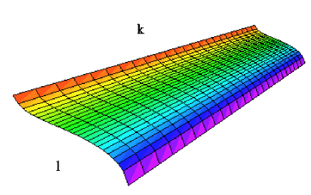
Figure 5: Profile with fixed-free BC in the transverse direction. In the computations, periodic BC are used in the longitudinal direction.

4.2 Application to random systems

In random systems, the conformal invariance prescriptions are recovered after disorder average chatelainberche98b ; igloirieger98 . The bulk critical properties of disordered Potts models have been investigated at criticality through conformal techniques by various authors picco97 ; cardyjacobsen97 ; jacobsencardy98 ; chatelainberche98b ; chatelainberche99 , using the longitudinal correlation function decay along periodic strips or the magnetization profiles in square-shaped systems with fixed boundary conditions along all the surfaces. Here, we consider the magnetization profiles of long strips with fixed-free boundary conditions in the transverse direction. Since a sufficient strip width is needed in order to apply the continuum limit conformal results in the transverse direction, TM techniques are useless (the strip width is limited to $L\leq 10$ using the connectivity TM) and MC simulations are preferred (with $L\leq 40$). The parameters used in this work for the MC simulations are given in Table 5. We mention that in spite of the large sizes used, the continuum limit is only approximately reached and perturbing effects will be expected close to the boundaries.

Table 5: Parameters for the MC simulations at criticality. The same parameters are used for all values of $q$. The number of disorder realizations is increased at larger sizes. At each disorder realization, 1000 MC sweeps are discarded and 5000 MC sweeps are used to compute physical quantities.

$L$	$K$	# of realizations
10	100, 200, 300, 400 and 500	1000
14	100, 200, 300, 400 and 500	1000
18	138, 277, 555 and 833	1000
24	80 and 96	1000
	192, 384 and 500	4000
30	100 and 200	1000
	300, 400 and 500	4000
40	100 and 200	1000
	300, 400 and 500	4000

Examples of profiles with fixed-free BC are shown in Figure 6 for $q=3$ and 8 for different strip lengths $K$ at a fixed width $L=40$. The influence of the length $K$ of the strip becomes negligible when $K\geq 300$.

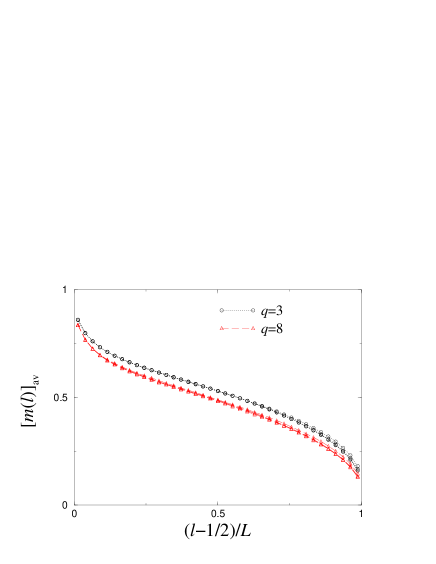
Figure 6: Profile with fixed-free BC for two values of $q$. The size $L\times K$ of the strips of width $L=40$ ranges between $40\times 200$ (upper profiles) and $40\times 500$ (lower profiles), and average was performed over 1000 to 4000 realizations of disorder. Error bars are smaller than the symbols.

Introducing the variable $\zeta=\frac{l-1/2}{L}$ in equations (11) and (12), one thus expects the following behaviour:

$$[m(\zeta)]_{\rm av}={\cal A}(\pi/L)^{x_{b}}\times[\sin\pi\zeta]^{-x_{b}}\times[\cos\pi\zeta/2]^{x_{1}}.$$ (13)

In order to simplify the following expressions, we introduce the functions $f(\zeta)=\sin\pi\zeta$ and $g(\zeta)=\cos\pi\zeta/2$, and the ratio

$$R(\zeta,\zeta^{\prime})=\frac{[m(\zeta)]_{\rm av}}{[m(\zeta^{\prime})]_{\rm av}}.$$ (14)

Since $f(\zeta)$ is symmetric with respect to the middle of the strip $\zeta=\frac{1}{2}$, the surface dimension $x_{1}$ can be deduced from local symmetric values of the profile:

$$R(\zeta,1-\zeta)=\left[\frac{g(\zeta)}{g(1-\zeta)}\right]^{x_{1}}=[\cot\pi\zeta/2]^{x_{1}},$$ (15)

or

$$x_{1}=\frac{\ln R(\zeta,1-\zeta)}{\ln[\cot\pi\zeta/2]}.$$ (16)

Examples of effective surface scaling dimensions, according to Equation (16), are shown in Figure 7 for $q=4$ with 4000 different configurations of couplings for strips of width $L=40$ and increasing lengths from $K=100$ to 500.

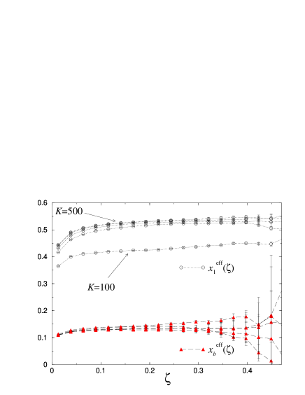
Figure 7: Examples of effective surface and bulk scaling dimensions for $q=4$ and a disorder amplitude $r^{\star}=7$. The size of the strip are $40\times K$, with $K=100$, 200, …, 500. Between $K=300$ and 500, the effective exponents remain constant up to the accuracy of the computations. Average was performed over 1000 to 4000 realizations of disorder.

In the thermodynamic limit, these scaling dimensions should be unambiguously determined for any value of the position $\zeta$ in the transverse direction of the strip. In practice, due to the finite size of the system and to lattice effects close to the boundaries , equation (16) defines effective quantities $x_{1}(\zeta,L)$ which do depend on the position $\zeta$ along the strip, and also on the strip width and evolve towards the right limit when $L\to\infty$. As it was already visible in Figure 6, between $K=300$ and $K=500$, the strip length can be considered to be long enough in order to avoid finite-size effects in the long direction. For these strip lengths, one can also observe a plateau in Figure 7 where there is no significant variation of the the effective exponents which remain almost constant in the region $\zeta=0.20-0.35$, and whose extrapolated values should be consistent. The values computed in the plateau region are thus studied as $L$ increases and extrapolation is made towards the thermodynamic limit $L\to\infty$. The dependence of the effective exponents on the strip width is shown in Figure 8 for $\zeta=0.25$. A linear extrapolation leads to the estimations of $x_{1}(\zeta,\infty)$, collected in Table 6. The results exhibit a good stability relative to the position $\zeta$ and allow a final determination of the scaling dimension $x_{1}$, given in the last column of the table. On the other hand, we observe important corrections to scaling in the boundary behaviour, since the surface exponent falls down rapidly as $\zeta\to 0$. This effect is the possible origin of the discrepancy with the boundary scaling dimension found in Ref. chatelainberche98 for $q=8$: $x_{1}\simeq 0.47$, which is recovered here in the limit $\zeta\to 0$.

Figure 8: Effective surface exponent at $\zeta=0.25$ plotted against $L^{-1}$. The intercept corresponds to the extrapolated value in the thermodynamic limit: $x_{1}(0.25,\infty)$.

Table 6: Extrapolation in the thermodynamic limit of the scaling dimension of the surface magnetization, $x_{1}(\zeta,\infty)$, measured at different values of $\zeta$. The last column presents our definitive determination for each value of $q$.

		$\zeta$
$q$	$r^{\star}$	$\zeta\to 0$	0.20	0.25	0.30	$x_{1}$
3	5	0.438(1)	0.518(1)	0.526(2)	0.525(3)	0.523(2)
4	7	0.453(1)	0.541(2)	0.553(2)	0.552(3)	0.549(2)
6	8	0.478(1)	0.567(2)	0.577(2)	0.574(4)	0.573(3)
8	10	0.482(1)	0.577(2)	0.588(3)	0.588(5)	0.584(3)

For the bulk exponent, using the quantity

$$R(\zeta,1/2)=[f(\zeta)]^{-x_{b}}[\sqrt{2}g(\zeta)]^{x_{1}},$$ (17)

we can form a combination where $x_{1}$ cancels, leading to:

$$x_{b}= \{\ln R(\zeta,1/2)\times\ln[\sqrt{2}g(1-\zeta)]$$

$$-\ln R(1-\zeta,1/2)\times\ln[\sqrt{2}g(\zeta)]\}$$

$$\times\left\{\ln[f(\zeta)]\times\ln\left[\frac{g(\zeta)}{g(1-\zeta)}\right]\right\}^{-1}.$$

This expression involves three points of the profile and is thus subject to stronger numerical fluctuations than the surface scaling dimension, as shown in Figure 7. Unfortunately, compared to previous precise determinations, no accurate extrapolation can be made here. One can however check the conformal expression (13). For that purpose, it is necessary to extrapolate the rescaled profiles $[m_{L}(\zeta)]\times L^{x_{b}}$, obtained at finite sizes, towards the thermodynamic limit. Considering, as we did before, that the longer strips are large enough to be unaffected by finite-size effects in the long direction, extrapolation to infinite width $L$ only will be done. For each position $\zeta$ in the transverse direction, we plot the corresponding local magnetization as computed for different strip widths and then extrapolate in the limit $L\to\infty$. Examples of linear and quadratic least square fits are shown in Figure 9. The latter one has been preferred.

Figure 9: Extrapolation to infinite width of the profiles. The solid lines corresponds to $q=8$ and the dashed lines to $q=3$. Two fitting curves are presented (for $\zeta=0.25$, $q=3$), a least square linear fit (dotted line) and quadratic (solid line). The quadratic fit is more accurate.

Figure 10: Rescaled profiles at different strip widths for $q=8$ (open symbols) and extrapolation to $L\to\infty$ (full circles). The solid line is the conformal expression where the amplitude is the only free parameter. The agreement between the extrapolated data and the conformal profile is very good.

It leads to an extrapolated profile, which is compared to the conformal expression in Figure 10 for $q=8$. In the conformal formula, the scaling dimensions of Tables 3 and 6 are entered and the amplitude is the only free parameter. In spite of the small strip widths considered, the extrapolation procedure introduced in Fig. 9 is very accurate, since the agreement between extrapolated data (full circles) and Eq. 13 (solid line) is fairly satisfactory. This is a strong evidence which supports the validity of the conformal expression for the profile.

5 Multifractal behaviour at criticality

In this section, we study the possible multifractal behaviour at the critical point and consider different moments for the magnetization profile, $[m^{n}(l)]^{1/n}_{\rm av}$, and that of the correlation function $[G_{\sigma}^{n}(r)]^{1/n}_{\rm av}$. The characteristic exponents, $x_{b}^{(n)}$ and $x_{1}^{(n)}$, in the bulk and at the surface, respectively, are expected to vary with $n$ for multifractal behaviour. Indeed, it was first Ludwig ludwig87 who predicted multifractality in the bulk correlation function of the random bond Potts model by conformal perturbative methods (see also the results by Lewis in Refs. lewis98 ; lewis99 ), which was confirmed recently by Olson and Young olsonyoung99 by MC simulations in the square geometry. Here we rather work in the strip geometry and calculate both the bulk and surface scaling exponents.

The calculations about the moments of the critical profile are parallel with that in the previous section and the scaling dimensions are extracted from the expected functional form:

$$[m^{n}(\zeta)]_{\rm av}^{1/n}={\cal A}(\pi/L)^{x_{b}^{(n)}}\times[\sin\pi\zeta]^{-x_{b}^{(n)}}\times[\cos\pi\zeta/2]^{x_{1}^{(n)}}\;,$$ (19)

which is analogous to (13) for the average behaviour, i.e. for $n=1$. We note that the typical behaviour corresponds to $n=0$,i.e. $\exp[\ln m(\zeta)]_{\rm av}$.

In the actual calculation we have considered the $q=8$ model on strip-like samples with $K=500$ and $L=10,20,30$ and $40$ and the average is performed over $5000$ realizations. Using the method of the previous section first we deduced from equation (19) the effective, size and position dependent surface scaling dimensions, $x_{1}^{(n)}(\zeta,L)$, which are then extrapolated to the thermodynamic limit, $L\to\infty$. The extrapolation procedure is demonstrated in Figure 11, whereas the extrapolated data are presented in Table 7. As one can see in this Table the critical point surface magnetization of the random bond Potts model shows multifractal behaviour: The scaling dimensions of the different moments of the surface magnetization, $x_{1}^{(n)}$, are monotonously decreasing with $n$. Note that for $n=2$ the surface scaling dimension is very close to the pure (and random) Ising value of $x_{1}=1/2$.

Figure 11: Effective surface dimensions of the $n^{\rm th}$-order moments of the magnetization profile, evaluated at $\zeta=0.25$ for $q=8$ and $n=0$, 1, 2, 3. Dashed lines denote results of quadratic extrapolation.

Table 7: Extrapolation in the thermodynamic limit of the scaling dimension associated to the moments of the surface magnetization and measured at different values of $\zeta$ ($q=8$). The last row presents our definitive determination.

	$\zeta$
$n$	$0.20$	$0.25$	$0.30$	$0.35$	$x_{1}^{(n)}$
0	0.601(7)	0.600(7)	0.602(9)	0.599(11)	0.600(9)
1	0.585(5)	0.582(6)	0.582(8)	0.579(11)	0.582(8)
2	0.496(3)	0.496(4)	0.500(6)	0.498(8)	0.498(5)
3	0.387(11)	0.384(14)	0.384(18)	0.381(25)	0.384(17)

Next we turn to study the multifractal behaviour of the bulk magnetization. As mentioned in the previous section, from the magnetization profiles in finite strips one cannot extract precise estimates for the scaling dimension $x_{b}^{(n)}$. Therefore we used a different technique, based on the Blöte and Nightingale connectivity transfer matrix blotenightingale82 . Since transfer operators in the time direction do not commute in disordered systems, the free energy density is defined by the leading Lyapunov exponent. For an infinitely long strip of width $L$ with periodic boundary conditions, the leading Lyapunov exponent is given by the Furstenberg method furstenberg63 :

$$\Lambda_{0}(L)=\lim_{m\to\infty}\frac{1}{m}\ln\left|\!\left|\left(\prod_{j=1}^{m}{\bf T}_{j}\right)\mid\!v_{0}\rangle\right|\!\right|,$$ (20)

where ${\bf T}_{j}$ is the transfer matrix and $\mid\!v_{0}\rangle$ is a unit initial vector. The free energy density is thus given by $[f_{0}(L)]_{\rm av}=-L^{-1}\Lambda_{0}(L)$. For a specific disorder realization, the spin-spin correlation function along the strip

$$G_{\sigma}(k)=\frac{q\langle\delta_{\sigma_{l,1}\sigma_{l,k+1}}\rangle-1}{q-1},$$ (21)

follows from the application of products of transfer matrices on the ground state eigenvector associated to $\Lambda_{0}$ (for details see, e.g. Ref. chatelainberche99 ).

We will now assume that conformal covariance can be applied to the order parameter correlation function and its moments. In the infinite complex plane $z=x+{\rm i}y$ the correlation function exhibits the usual algebraic decay at the critical point $[G_{\sigma}^{n}(\rho)]_{\rm av}^{1/n}={\rm const}\times\rho^{-2x_{b}^{(n)}},$ where $\rho=\mid\!z_{1}-z_{2}\!\mid$. Under the logarithmic transformation $w=\frac{L}{2\pi}\ln z=k+{\rm i}l$ , one gets the usual exponential decay along the strip $[{G}_{\sigma}^{n}(k)]_{\rm av}^{1/n}={\rm const}\times\exp\left(-\frac{2\pi}{L}x_{b}^{(n)}k\right)$ (see Fig. 12 for an illustration). The scaling dimension $x_{b}^{(n)}$ can thus be deduced from an exponential fit.

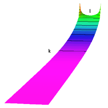
Figure 12: Spin-spin correlation function on a long strip with periodic BC in the transverse direction (the upper left corner also corresponds to the upper right corner). This Figure is a 3D plot where the value of the correlation function between the origin (upper left corner) and any lattice site $(k,l)$ is plotted on a vertical axis at position $(k,l)$.

This method was used in Ref. chatelainberche99 for the average correlation function, i.e. for $n=1$. In this work, we calculate the higher moments, as well as the typical behaviour, which corresponds to $n=0$.

For each strip size ($L=2-8$), we considered systems of length $\sim 10^{6}$ and an average is performed over $80\times 10^{3}$ disorder configurations. For a given strip the effective, size-dependent exponents follow from a linear fit in a semi-log plot, as exemplified in Figure 13. It is clearly seen that the scaling dimensions are different for the different moments of the spin-spin correlation function. The effective exponents are then extrapolated as $L\to\infty$ and the estimated values are presented in Table 8 for different values of $q$ (at $r^{\star}(q)$).

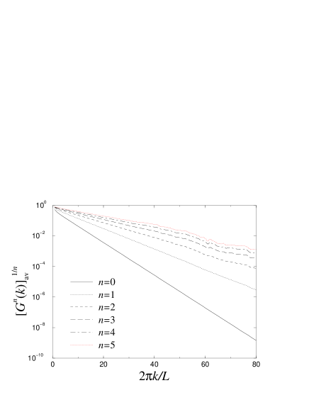
Figure 13: Moments of the spin-spin correlation function (semi-log scale) for $q=8$, $L=7$.

Table 8: Scaling dimensions of the moments of the spin-spin correlation function computed at $r=r^{\star}$.

	$x_{b}^{(n)}$
$n$	$q=3$	$q=4$	$q=6$	$q=8$
0	0.154(1)	0.177(1)	0.207(1)	0.234(1)
1	0.132(1)	0.138(1)	0.146(1)	0.150(1)
2	0.116(1)	0.114(1)	0.114(1)	0.112(1)
3	0.104(1)	0.097(1)	0.094(2)	0.091(2)
4	0.095(2)	0.087(2)	0.081(2)	0.077(2)
5	0.088(2)	0.079(2)	0.072(2)	0.068(2)

Again the critical point bulk magnetization shows multiscaling behaviour, for all $q\geq 3$ the scaling dimensions, $x_{b}^{(n)}$, are monotonously decreasing with $n$. One can make a comparison with perturbative results:

$$x_{b}^{(n)}=x_{b}^{p}-\frac{9}{32}(n-1)\left[\frac{2}{3}\epsilon+(A+B(n-2))\epsilon^{2}+O(\epsilon^{3})\right],$$ (22)

where $x_{b}^{p}$ is the bulk exponent in the pure model, $\epsilon$ is a small expansion parameter related to the deviation of the pure model’s central charge to that of the Ising model ($\epsilon=2/15$ and $1/3$ for $q=3$ and 4, respectively lewis99 ), and $A=11/12-4\ln 2$ and $B=\frac{1}{24}(33-29\sqrt{3}\pi/3)$ are numerical factors. The first-order term in Eq. (22) is due to Ludwig ludwig87 and the second-order term to Lewis lewis98 . This result is known to be valid close to $q=2$ and for the lower moments. The comparison with our data is made in Table 9. One can observe a good agreement with the result of Lewis for $q=3$, especially for the lower moments. For $q=4$, the perturbation expansion probably breaks down already at $n=3$, since $x_{b}^{(3)}$ is found to be larger than $x_{b}^{(2)}$ with the formula of Lewis. It is remarkable that the second-order term in the perturbation expansion vanishes at $n=2$, which could explain the stability of the exponent associated to the second moment, with respect to variations of $q$, has already been noticed by Olson and Young olsonyoung99 .

Table 9: Scaling dimensions of the moments of the spin-spin correlation function computed at $r=r^{\star}$. The numerical estimates on the first column are compared to the results of the 1st and 2nd order perturbation theory in Eq. (22).

	$x_{b}^{(n)}$ for the 3-state Potts model
$n$	num.	1st order	2nd order
0	0.154(1)	0.158	0.157
2	0.116(1)	0.108	0.118
3	0.104(1)	0.083	0.110
	$x_{b}^{(n)}$ for the 4-state Potts model
$n$	num.	1st order	2nd order
0	0.177(1)	0.188	0.181
2	0.114(1)	0.063	0.120
3	0.097(1)	0.000	0.167

We close this section by presenting different moments of the magnetization profile, $[m^{n}(l)]_{\rm av}^{1/n}$, as extrapolated towards $L\to\infty$. In Figure 14 two moments ($n=0$ and $n=2$) of the scaled profiles are plotted for the $q=8$ model, where the open symbols represents the finite-width data. The extrapolated profile, denoted by full circles is in perfect agreement with the conformal results in equation (19), where the scaling dimensions $x_{b}^{(n)}$ and $x_{1}^{(n)}$ are taken from Tables 8 and 10, respectively, and the only fitting parameter is the amplitude in equation (19). We consider this agreement as a strong evidence in favour of the validity of the conformal expression for the averaged moments of the order parameter profile.

Figure 14: Rescaled $n^{\rm th}$-order profiles at different strip widths for $q=8$ (open symbols) and extrapolation to $L\to\infty$ (full dots). The solid line is the conformal expression with only the amplitude as a free parameter.

6 Discussion

In this paper the critical behaviour of the two-dimensional random bond Potts model is studied by MC simulations, transfer matrix techniques and conformal methods. New features of our present work are the following. i) For the first time we have investigated the surface critical behaviour of the model and determined the surface magnetization critical exponent, $\beta_{1}$, from approach to criticality. In addition we got estimates for the corresponding bulk exponent, $\beta$. ii) We have studied the critical point magnetization profiles in strip-like geometries and deduced the scaling dimension $x_{1}=\beta_{1}/\nu$ from the predictions of conformal invariance. iii) We have presented numerical evidence for the multifractal behaviour of the surface and bulk magnetizations at the critical point and the scaling dimensions of the averaged moments, $x_{b}^{(n)}$ and $x_{1}^{(n)}$ are calculated. iv) Finally, we have demonstrated that the different moments of the critical magnetization profiles, as well as the correlation function obey conformal invariance.

The critical exponents and the scaling dimensions of the average quantities are continuously varying functions of $q$, however an exponent relation $4\beta=\beta_{1}$ is approximately satisfied, as can be observed in Table 3. The anomalous dimensions of the relevant scaling fields in equations (1) and (2) can be estimated using the scaling relations: $y_{t}=1/\nu=x_{b}/\beta=x_{1}/\beta_{1}$, $y_{h}=2-x_{b}$, and $y_{h_{s}}=1-x_{1}$. Their values are presented in Table 10. While $y_{t}$ remains close to 1 (but $\nu$ satisfies the limit $\nu\geq 2/d$ chayesetal ) for all values of $q$, the anomalous dimensions related to the magnetic field vary with $q$.

Table 10: Anomalous dimensions of the relevant bulk and surface scaling fields.

$q$	$r^{\star}$	$x_{b}/\beta$	$x_{1}/\beta_{1}$	$2-x_{b}$	$1-x_{1}$
3	5	0.971(29)	0.965(6)	1.868(3)	0.477(2)
4	7	0.979(35)	0.979(13)	1.862(3)	0.451(2)
6	8	0.980(40)	0.986(18)	1.854(3)	0.427(3)
8	10	0.993(26)	0.978(18)	1.849(3)	0.416(3)

- (1)
- (2)
- (3) A.B. Harris, J. Phys. C 7, 1671 (1974).
- (4) B.N. Shalaev, Phys. Rep. 237, 129 (1994).
- (5) W. Selke, L.N. Shchur and A.L. Talapov, in Annual Reviews of Computational Physics, edited by D. Stauffer (World Scientific, Singapore, 1994), Vol 1 p. 17.
- (6) Y. Imry and M. Wortis, Phys. Rev. B 19, 3580 (1979).
- (7) M. Aizenman and J. Wehr, Phys. Rev. Lett. 62, 2503 (1989).
- (8) K. Hui and A.N. Berker, Phys. Rev. Lett. 62, 2507 (1989).
- (9) F.Y. Wu, Rev. Mod. Phys. 54, 235 (1982).
- (10) A.W.W. Ludwig, Nucl. Phys. B 285 [FS19], 97 (1987).
- (11) A.W.W. Ludwig and J.L. Cardy, Nucl. Phys. B 330 [FS19], 687 (1987).
- (12) A.W.W. Ludwig, Nucl. Phys. B 330, 639 (1990).
- (13) Vl. Dotsenko, M. Picco and P. Pujol, Nucl. Phys. B 455 [FS], 701 (1995).
- (14) G. Jug and B.N. Shalaev, Phys. Rev. B 54, 3442 (1996).
- (15) V.S. Dotsenko, Physics-Uspekhi 38, 457 (1995).
- (16) S. Wiseman and E. Domany, Phys. Rev. E 51, 3074 (1995).
- (17) M. Picco, Phys. Rev. B 54, 14 930 (1996).
- (18) J.K. Kim, Phys. Rev. B 53, 3388 (1996).
- (19) S. Chen, A.M. Ferrenberg and D.P. Landau, Phys. Rev. Lett. 69, 1213 (1992).
- (20) S. Chen, A.M. Ferrenberg and D.P. Landau, Phys. Rev. E 52, 1377 (1995).
- (21) C. Chatelain and B. Berche, Phys. Rev. Lett. 80, 1670 (1998).
- (22) F. Yaşar, Y. Gündüç, and T. Çelik, Phys. Rev. E 58, 4210 (1998).
- (23) M. Picco, e-print cond-mat/9802092.
- (24) T. Olson and A.P. Young, e-print cond-mat/9903068.
- (25) M. Picco, Phys. Rev. Lett. 79, 2998 (1997).
- (26) J.L. Cardy and J.L. Jacobsen, Phys. Rev. Lett. 79, 4063 (1997).
- (27) J.L. Jacobsen and J.L. Cardy, Nucl. Phys. B 515, 701 (1998).
- (28) C. Chatelain and B. Berche, Phys. Rev. E 58, R6899 (1998).
- (29) C. Chatelain and B. Berche, e-print cond-mat/9902212.
- (30) K. Binder, in Phase Transitions and Critical Phenomena, edited by C. Domb and J.L. Lebowitz (Academic Press, London, 1983),Vol. 8, p. 1.
- (31) W. Selke, F. Szalma, P. Lajkó, and F. Iglói, J. Stat. Phys. 89, 1079 (1997).
- (32) F. Iglói, P. Lajkó, W. Selke, and F. Szalma, J. Phys. A: Math. Gen. 31, 2801 (1998).
- (33) F. Szalma and F. Iglói, J. Stat. Phys. **, ** (1999).
- (34) W. Janke, in Computational Physics: Selected Methods - Simple Exercises - Serious Applications, edited by K.H. Hoffmann and M. Schreiber (Springer, Berlin, 1996).
- (35) G.T. Barkema and M.E.J. Newmann, in Monte Carlo Methods in Chemical Physics, Advances in Chemical Physics 105 edited by D. Ferguson, J. I. Siepmann, and D. G. Truhlar (Wiley, New York, 1999).
- (36) P.W. Kasteleyn and C.M. Fortuin, J. Phys. Soc. Japan 26 Suppl., 11 (1969).
- (37) R.H. Swendsen and J.S. Wang, Phys. Rev. Lett. 58, 86 (1987).
- (38) U. Wolff, Phys. Rev. Lett. 62, 361 (1989).
- (39) Vl. Dotsenko, J.L. Jacobsen, M.A. Lewis, and M. Picco, e-print cond-mat/9812227.
- (40) E. Carlon and F. Iglói, Phys. Rev. B 57, 7877 (1998).
- (41) J. Salas and A.D. Sokal, J. Stat. Phys 88, 567 (1997).
- (42) A. Aharony and A.B. Harris, Phys. Rev. Lett. 77, 3700 (1996).
- (43) B. Derrida, Phys. Rep. 103, 29 (1984).
- (44) S. Wiseman and E. Domany, Phys. Rev. Lett. 81, 22 (1998).
- (45) S. Wiseman and E. Domany, Phys. Rev. E 58, 2938 (1998).
- (46) M. E. Fisher and P. G. de Gennes, C. R. Acad. Sci. Paris B 287, 207 (1978).
- (47) T.W. Burkhardt and T. Xue, Phys. Rev. Lett. 66, 895 (1991).
- (48) F. Iglói and H. Rieger, Phys. Rev. B 57, 11 404 (1998).
- (49) M.A. Lewis, Europhys. Lett. 43, 189 (1998).
- (50) M.A. Lewis, e-print cond-mat/9905401.
- (51) H.W.J. Blöte and M.P. Nightingale, Physica (Amsterdam) 112A, 405 (1982).
- (52) H. Furstenberg, Trans. Am. Math. Soc. 108, 377 (1963).
- (53) J.T. Chayes, L. Chayes, D.S. Fisher and T. Spencer, Phys. Rev. Lett. 57, 2999 (1986).