Critical Behavior of the Random Potts Chain

Abstract

We study the critical behavior of the random $q$-state Potts quantum chain by density matrix renormalization techniques. Critical exponents are calculated by scaling analysis of finite lattice data of short chains ($L\leq 16$) averaging over all possible realizations of disorder configurations chosen according to a binary distribution. Our numerical results show that the critical properties of the model are independent of $q$ in agreement with a renormalization group analysis of Senthil and Majumdar (Phys. Rev. Lett.76, 3001 (1996)). We show how an accurate analysis of moments of the distribution of magnetizations allows a precise determination of critical exponents, circumventing some problems related to binary disorder. Multiscaling properties of the model and dynamical correlation functions are also investigated.

I Introduction

The study of the critical properties of systems subject to quenched randomness is of great interest because of its relevance for many experimental systems. This is a challenging research area which has been quite active in the last decades. One has witnessed a growing interest in understanding the effect of randomness (bond and site disorder), since Harris showed that disorder is a relevant perturbation in a system undergoing a second order phase transition when the exponent $\alpha$ of the specific heat in the pure system is positive.[1] In this context the two dimensional Ising model has attracted considerable interest, since the Onsager singularity of the specific heat ($\alpha=0$) makes the Harris criterion inconclusive (for a review, see e.g. Ref. [2]). Renormalization group studies,[3] supported by Monte Carlo simulations,[4] established that homogeneous disorder is marginally irrelevant, i.e. it does not modify the critical behavior of the system, except for the appearance of logarithmic corrections.

In accordance with the Harris criterion, randomness is on the other hand a relevant perturbation for the $q=3$ and $q=4$ Potts models. Furthermore, an infinitesimal amount of disorder was shown to turn the first order phase transition of the $q>4$ Potts model into a second order one.[5, 6, 7] Numerical estimates of the critical exponents for an homogeneous disorder indeed showed a monotonic increase of the magnetization exponent $\beta$ with the value $q$ while the thermal exponent $\nu$ remains constant within numerical accuracy.[8, 9, 10, 11] Thus for the two dimensional classical Potts model, homogeneous disorder gives rise to several different universality classes dependent on the value of $q$.

Other systems with quenched randomness which have been investigated in the past years are quantum spin chains. The interest in these models has grown considerably after a remarkable paper of Fisher [12] who derived many of the critical properties of the random transverse Ising chain (RTIC) using a real space renormalization-group scheme which is claimed to be asymptotically exact. His predictions were checked numerically by several authors, using the mapping of the RTIC onto a free fermion model,[13] density-matrix renormalization group [14] (DMRG) or quantum Monte Carlo.[15] Critical exponents calculated numerically were found in good agreement with Fisher’s results. The renormalization scheme of Fisher was also applied to the $q$-state disordered Potts chain by Senthil and Majumdar;[16] they found that the critical behavior does not depend on $q$, therefore all critical exponents should be identical to those of the RTIC obtained by Fisher and corresponding to the case $q=2$. We recall that the disordered quantum Potts chain is equivalent to a two dimensional classical Potts model with correlated disorder (analogous to the McCoy-Wu model [17] corresponding to $q=2$), where the quantum formulation is obtained from the classical one in the extreme anisotropic limit.[18] The conclusion of a unique universality class is thus different from what found in the classical Potts model with homogeneous disorder discussed above.

In this paper, we check the predictions of a unique universality class, independent of the number of states $q$, by studying bulk and surface magnetization properties. We consider both the regimes $q\leq 4$ and $q>4$, where the pure model exhibits a second and first-order transition, respectively. We also report an investigation of the multiscaling behavior of the magnetization, which strongly supports the asymptotic expression for the probability distribution found by Fisher in the RTIC case. The dynamical behavior is considered through the decay of the spin-spin correlation function along the time direction. All numerical results are obtained by density matrix renormalization group techniques,[19, 20] applied to the two dimensional classical Potts model with correlated disorder. We use Nishino’s [21] version of White’s DMRG algorithm,[19] where one renormalizes classical transfer matrices. The exponents are calculated from finite size scaling analysis of finite lattice data for chains of lengths $L\leq 16$ with exact enumeration over all possible ($2^{L}$) disorder realizations, obtained from a binary distribution. The justification for this type of approach will be presented in more detail in the text.

Our numerical results are fully consistent with the conclusion of Senthil and Majumdar,[16] i.e. the $q$-state Potts model has critical properties which do not depend on $q$. Moreover, dynamical properties which are not accessible by Fisher’s renormalization group, do not seem to depend on $q$.

The paper is organized as follows: In Sec. II, the model is presented and we give a justification for the choice of the numerical methods that are used. Section III is devoted to the estimates of the critical exponents. Multi-fractality is investigated in Sec. IV. The dynamical spin-spin correlation functions are studied in Sec. V. Finally, a brief summary and an outlook will be presented in Sec. VI.

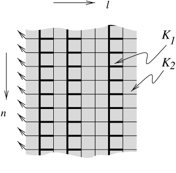
FIG. 1.: Layered structure of the model with coupling constants $K_{1}$ and $K_{2}$ taken from the distribution (2) and indicated by thick and thin bonds, respectively. The arrows on the left indicate fixed boundary conditions, while spins on the right surface are left free.

II Model and numerical methods

We consider a randomly layered (see Fig. 1) two-dimensional classical $q$-state Potts model on a square lattice. The model is defined by the Hamiltonian

$$-\beta{\cal H}=\sum_{l=1}^{L}K_{l}\sum_{n}\left[\delta_{\sigma_{l,n},\sigma_{l+1,n}}+\delta_{\sigma_{l,n},\sigma_{l,n+1}}\right],$$ (1)

where the spins can take the values $\sigma_{l,n}=0,\ldots,q-1$ and the exchange couplings $K_{l}$ are randomly chosen according to the binary distribution

$${\cal P}(K_{l})={1\over 2}\left[\delta(K_{l}-K_{1})+\delta(K_{l}-K_{2})\right].$$ (2)

Since the model is equivalent to the random quantum Potts chain studied by Senthil and Majumdar,[16] we use the quantum chain’s vocabulary. In the case $q=2$, the system reduces to the RTIC.

The particular arrangement of coupling constants, i.e. the fact that vertical couplings are identical to adjacent horizontal couplings to their right side (see Fig. 1), and that both couplings $K_{1}$ and $K_{2}$ have equal probabilities (see Eq. (2)), makes the model self-dual. The location of the critical point is known exactly:[22]

$$\left(e^{K_{1}}-1\right)\left(e^{K_{2}}-1\right)=q.$$ (3)

The strength of the disorder is monitored by the ratio $r=K_{1}/K_{2}$, $r=1$ corresponding to the pure model.

Although the DMRG method is capable of dealing with very large systems (of few hundreds of sites) with remarkable accuracy, some care has to be taken when working with disordered systems. The infinite lattice version of the algorithm is known to give incorrect results,[23] especially at strong disorder; it is essential [24] when dealing with inhomogeneous systems to use the finite lattice DMRG algorithm [19] which is designed to determine accurately properties of finite systems (In our calculations we typically used three full sweeps through the lattice). It is furthermore well known that due to the lack of self-averaging,[25, 26] an insufficient number of samples yields a wrong estimation of the average over randomness and might lead to typical values instead of the expected average quantities.[27] As we aim to an accurate determination of critical exponents, we have chosen to restrict ourselves to relatively narrow strips ($L\leq 16$ which turns out to be large enough, since corrections to scaling will appear very small) for which we were able to do an exact enumeration over all disorder realizations. As the system size is small compared to typical DMRG calculations a limited number of states kept ($m\leq 16$) is sufficient to obtain accurate results.

The setup of the calculation follows Ref. [28], where the DMRG method was used to calculate exponents and magnetization profiles for the pure Potts model. The $Z_{q}$-symmetry of the Potts model has been broken by introducing fixed–free boundary conditions: We fixed the spin at one edge of the system to a value $\sigma_{0,n}=0$, while at the other edge the spin is free. This type of boundary conditions induces a finite magnetization in the system [29] from which surface and bulk critical exponents can be calculated using finite size scaling analysis.

Figure 2 shows magnetization profiles (defined by Eq. (4)) of $10$ samples for the three-state Potts model with $L=16$ and with disorder amplitude $r=2$. Estimated error bars are much smaller than symbol sizes; averaging over all disorder realizations produces the smooth profiles shown in Fig. 4. In this procedure the only source of error comes from the truncation on the DMRG basis, this error is quite small even for $m=16$ states kept as we restricted ourselves to small systems.

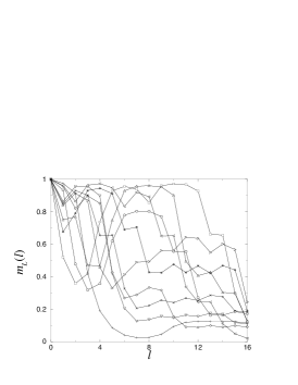
FIG. 2.: Magnetization profiles for ten random configurations of exchange couplings at $q=3$, $r=2$, $L=16$. Error bars are smaller than the symbols.

III Critical exponents

A Finte-Size scaling

We used the standard order parameter of the Potts model:

$$\left[m_{L}(l)\right]_{\rm av}={q\left[\langle\delta_{\sigma_{l,n},0}\rangle\right]_{\rm av}-1\over q-1},$$ (4)

where $\langle\dots\rangle$ denotes the thermal average and $\left[\dots\right]_{\rm av}$ the average over randomness. Standard finite size techniques have been used to estimate the bulk and surface critical exponents

$$[m_{L}^{b}]_{\rm av}\sim L^{-x_{b}},\quad[m_{L}^{s}]_{\rm av}\sim L^{-x_{1}},$$ (5)

where we have defined $[m_{L}^{b}]_{\rm av}\equiv[m_{L}(L/2)]_{\rm av}$ and $[m_{L}^{s}]_{\rm av}\equiv[m_{L}(L)]_{\rm av}$, which are the average magnetizations in the middle of the strip and at the free edge. From finite size data we calculated the approximants, defined as

$$x_{b}(L)=-{\ln[m_{L+1}^{b}]_{\rm av}-\ln[m_{L-1}^{b}]_{\rm av}\over\ln(L+1)-\ln(L-1)}$$ (6)

in the bulk case and similarly for the surface approximants. In the limit $L\to\infty$ the approximants scale towards the bulk and surface exponents $x_{b}$ and $x_{1}$.

Table I reports the finite size approximants for the surface exponents for various values of $q$ and of disorder ratios $r$. The extrapolation towards the thermodynamic limit was done using the BST algorithm.[30] The boundary magnetization exponent, $x_{1}$, exhibits a striking convergence for all values of $q$ and all disorder amplitudes, but for crossover effects discussed below. It is clearly independent of $q$, and in good agreement with the RTIC value $x_{1}=1/2$. The best numerical results are obtained for $q=2$, as the truncation error in the DMRG method is the smallest for this case, furthermore the surface exponent for the pure and disordered cases coincide for $q=2$ (they are both equal to $1/2$), therefore no crossover effects are to be expected.

TABLE I.: Approximants of the surface exponent for various $q$ and $r$. The last row shows the values extrapolated with the BST algorithm. We note that at $q=6$ the disorder amplitude being quite small, crossover effects from the pure model value $x_{1}=3$ slow down the convergence.

	$q=2$		$q=3$			$q=4$		$q=6$
$L$	$r=2$	$r=8$	$r=2$	$r=4$	$r=8$	$r=5$	$r=10$	$r=1.5$
5	0.41608413	0.44950692	0.46559328	0.46393358	0.46844808	0.47671724	0.47741488	0.55719868
7	0.43773154	0.46307866	0.48454642	0.47694537	0.47932515	0.48718127	0.48819610	0.56816316
9	0.45043349	0.47083067	0.49365387	0.48353868	0.48475158	0.49161650	0.49204019	0.56481411
11	0.45880966	0.47587114	0.49851791	0.48742293	0.48800690	0.49383119	0.49387188	0.56108433
13	0.46475540	0.47941816	0.50127872	0.48993505	0.49014411	0.49481028	0.49435771	0.54974464
15	0.46919708	0.48205234	-	0.49166836	0.49150054	-	-	-
$\infty$	0.50000(1)	0.5000(1)	0.498(4)	0.499(1)	0.500(1)	0.496(10)	0.50(5)	-

We recall that the values of the surface exponents for the pure Potts model are $x_{1}=2/3$ for $q=3$, $x_{1}=1$ for $q=4$ and $x_{1}=3$ for $q>4$. The last exponent has also been recently calculated by DMRG methods [31] (the surface transition is continuous even if the bulk has a first order transition). In the case $q=6$, $r=1.5$, one notices that the approximants approach the value $1/2$ in a non-monotonic fashion (the same situation occurs with $q=4$, $r=2$). This case corresponds to the weakest disorder considered and the non-monotonicity is most likely due to crossover effects from the exponent of the pure system ($x_{1}=3$). It is not possible to extrapolate the data in the last column of Table I with the BST method, since the largest size analyzed is still in the crossover region. However we can give an estimate of the exponent using the analysis of the moments presented in Section IV B; from such an analysis we find 0.49(3) in good agreement with the value of the RTIC, $1/2$. We also mention that calculations have been performed at $q=6$, $r=4$. The approximants then do not suffer from so strong crossover effects, an observation which supports the explanation given above.

Table II shows the approximants of the bulk exponent obtained from Eq. (6) for various $q$ and $r$. As it can be seen the approximants show a non-monotonic behavior, with oscillations which are stronger as the disorder ratio increases. These oscillations, which were already observed in the RTIC,[32] are due to the choice of a binary distribution of exchange couplings which introduces an energy scale $K_{1}-K_{2}$ in the problem; in other types of distributions, e.g. continuous ones, these oscillations are not present.[32]

Lattice extrapolation techniques, as the BST method, are not able to deal with oscillating corrections to scaling. We recall that the BST algorithm generates from an original series of $N$ approximants new series of $N-1$, $N-2$ …approximants at each iteration which are expected to have faster convergence towards the asymptotic value. In the BST analysis we found that even when starting from a monotonic series of data at weak disorder ratios, as in the cases $q=2$, $r=2$, the next series generated by the algorithm do not converge at all, but they show oscillating behavior. Therefore the BST method turns out to be useless in the analysis of the bulk exponent data. A better way to get a precise estimate of bulk exponent is based on the analysis of moments, which will be explained in Section IV B.

In any case the approximants of Table II for different values of $q$ are rather close to each other, which supports again the idea of $q$-independence of their values. We recall that for the pure Potts model the bulk exponent is $x_{b}=1/8$ for $q=2,4$ and $x_{b}=2/15$ for $q=3$. For $q>4$ the bulk transition is first order.

Fisher’s prediction for the bulk exponent is:[12]

$$x_{b}={3-\sqrt{5}\over 4}\approx 0.19098.\quad$$ (7)

Figure 3 shows a log-log plot of bulk magnetization vs. system size. The data correspond to different $q$ and $r$ and are all roughly parallel with slopes in the range $0.183-0.187$ indicated in the figure and obtained by a simple linear fit. In the scale of the figure oscillations are not visible and the estimated slopes correspond to the average of the approximants of Table II.

TABLE II.: Approximants of the bulk exponent for various $q$ and $r$.

	$q=2$		$q=3$			$q=4$		$q=6$
$L$	$r=2$	$r=8$	$r=2$	$r=4$	$r=8$	$r=5$	$r=10$	$r=1.5$
5	0.15352463	0.18540035	0.17119099	0.18598351	0.19697064	0.19644591	0.20327857	0.18415244
7	0.15902213	0.17126232	0.17606416	0.17698031	0.17098093	0.17386925	0.16655933	0.18858150
9	0.16285921	0.18653590	0.17971019	0.18728278	0.19301242	0.19257056	0.19639122	0.18942360
11	0.16572102	0.17921449	0.18137938	0.18203550	0.19536097	0.18054979	0.17782952	0.18957220
13	0.16802871	0.18804307	0.18299470	0.18816428	0.18974244	0.19214731	0.19569786	0.18635074
15	0.16991419	0.18254668	-	0.18411149	0.19515526	0.18319909	-	-

FIG. 3.: Power-law behavior of the bulk magnetization with the lattice size for several values of $q$ and $r$ (inset shows different disorder amplitudes for $q=4$). The values indicated correspond to a simple power-law fit.

We mention that, surprisingly, we observed a weak dependence of the effective critical exponents with the amplitude of disorder $r$ in the range $[2;20]$, while important cross-over effects with the strength of the disorder were observed, e.g. by Picco,[10] in the case of a two-dimensional Potts model with a homogeneous disorder. This is an evidence of the strongly attractive character of the random fixed point.

B Transverse magnetization profiles

Conformal invariance techniques are extremely accurate for studying second order phase transitions in isotropic pure systems. Conformal symmetry requires translation, rotation and scale invariance; obviously a single disorder realization does not have such properties, but it is plausible that conformal symmetry is restored after averaging over different disorder configurations. Indeed in recent investigations, conformal mappings of correlation functions and order parameter profiles have been successfully applied in two-dimensional systems with homogeneous disorder.[33] The case of correlated disorder, studied in this paper, is quite different as the system, even after disorder average, exhibits infinite anisotropy at the random fixed point (see Sec. V). Therefore conformal invariance should not hold. In spite of these restrictions, the magnetization profiles of the RTIC with fixed-free boundary conditions have been quite satisfactorily fitted with the conformal expression,[32], obtained e.g. by Burkhardt and Xue [34]

$$[m_{L}(l)]_{\rm av}={\cal A}(\pi/L)^{x_{b}}[\sin\pi\zeta]^{-x_{b}}[\cos\pi\zeta/2]^{x_{1}},$$ (8)

where $\zeta=(l-1/2)/L$. The success of such an approach probably results from the geometrical constraints induced by the strip shape of the system combined to scaling arguments: In this sense, if Eq. (8) turns out to be valid also for the disordered Potts chain, one should conclude that such a form of profile is not a strict consequence of conformal invariance, which does not hold in anisotropic critical systems,[35] but follows from more general grounds.

FIG. 4.: Magnetization profiles for several values of $q$ and $r$ (inset for $q=4$ and several disorder amplitudes) and the conformal expression with the Fisher exponents (solid line) with only the amplitude as a free parameter.

In this Section, we indeed ask the question whether Eq. (8) correctly describes the transverse magnetization profiles in the random Potts chain. Senthil and Majumdar [16] indeed argued that the scaling functions should be independent of $q$. The quantity $m(l)L^{x_{b}}$ being such a scaling function, if Eq. (8) holds in the RTIC chain when $L\to\infty$, it should also be valid in the same limit in the Potts case. Unfortunately, in our case, the largest strip being $L=16$, strong lattice effects make the fit to expression (8) impossible in practice (Fig. 4). The same observation was reported for the RTIC, but these finite-size effects vanish for the largest systems that can be reached using the free fermion mapping in the Ising case. If Eq. (8) is valid, the quantity

$$x_{1}(L)={\ln[m_{L}(3L/4)]_{\rm av}-\ln[m_{L}(L/4)]_{\rm av}\over\ln(\sqrt{2}-1)}$$ (9)

should converge towards the surface exponent $1/2$. The results are shown in Table III. This method cannot be considered as an exact determination of $x_{1}$ but it provides an indication of the possible validity of (8) for this system. The bulk exponent $x_{b}$ also follows from a three-point expression analogous to Eq. (9) and should be extracted from the magnetization profile, but our data are not accurate enough to allow this calculation.

TABLE III.: Approximants of the surface exponent for various $q$ and $r$ calculated with (9). The sizes in bold face correspond to chain for which there is a lattice point $l$ such that $(l-1/2)/L=1/4$, while the other data were obtained after fitting the finite-size profile. The results are compatible with the expected value of 0.5, seemingly supporting the expression of the transverse profile.

$L$	$q=2-r=8$	$q=3-r=4$	$q=4-r=5$	$q=6-r=4$
4	0.5161	0.5195	0.5505	0.5709
6	0.5094	0.5237	0.5494	0.5711
8	0.5039	0.5224	0.5411	0.5607
10	0.4996	0.5210	0.5341	0.5511
12	0.4995	0.5202	0.5314	0.5422
14	0.5010	0.5206	0.5310	0.5262
16	0.5000	0.5187	0.5269	-

IV Multi-fractality

A Probability distribution

According to Fisher, the probability distribution of the surface magnetization $m_{L}^{s}$ for a strip of width $L$ is expected to behave asymptotically as:

$${\cal P}(m_{L}^{s})\sim{1\over\sqrt{L}}\tilde{p}\left({\ln m_{L}^{s}\over\sqrt{L}}\right).$$ (10)

This expression was successfully used for the RTIC by Iglói and Rieger to rescale the probability distribution of the surface magnetization for several strips of different widths $L$ in Ref. [32]. The scaling function $\tilde{p}$ was found to have a power-law decay in the RTIC. Forgetting about the oscillations, the average behavior in Fig. 5 is compatible with this observation.

The results of Senthil and Majumdar [16] state that the scaling function $\tilde{p}$ is independent of $q$ in the thermodynamic limit. Here again, the widths of our strips are too small to give a smooth probability distribution, as shown in Fig. 5. The Figure shows that for the events which determine the average critical properties, i.e. those corresponding to the dominant contributions to the magnetization, the probability distribution is weakly dependent on $q$, in accordance with universality of Eq. (10). On the other hand, for the rare samples for which $m_{L}^{s}$ or $m_{L}^{b}\leq 10^{-5}$, Eq (10) breaks down. It is however possible to test expression (10) by analyzing the moments of the distribution.

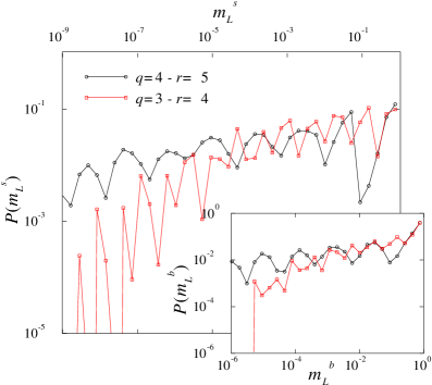
FIG. 5.: Probability distribution of the surface and bulk (inset) magnetizations defined with 64 bins ($q=3$ (squares) and $q=4$ (circles), $L=16$).

B Moments analysis

In this section we analyze moments of bulk and surface magnetization distributions. This analysis will help to avoid the problems related to the oscillations of the finite size estimates of the bulk exponent which, as shown in the previous section, hindered a reliable extrapolation of such quantity. Moments analysis was recently used in studies of self-organized critical systems.[36, 37] It was shown that such method provides an accurate means of investigation of subtle aspects that seem to emerge for such models.

In our case we are interested in the scaling of the asymptotic behavior of the moments. For instance, in the case of the surface or bulk magnetization we expect:

$${[{(m_{L})^{\omega}}}]_{\rm av}\sim L^{-\chi(\omega)}.$$ (11)

The exponent $\chi(\omega)$ generalizes the definitions of Eq.(6), which correspond to $\omega=1$. If the system is self-averaging, we expect a linear dependence of $\chi(\omega)$ with respect to $\omega$.[38] At a fixed size $L$, we consider the finite-size approximants of $\chi(\omega)$ defined as usual by:

$$\chi_{L}(\omega)=-\frac{\ln{[{(m_{L+1})^{\omega}}}]_{\rm av}-\ln{[{(m_{L-1})^{\omega}}]_{\rm av}}}{\ln(L+1)-\ln(L-1)}.$$ (12)

Plots of both quantities for $L=5,7,\ldots 15$ and $q=3$, $r=4$ are shown in Fig. 6. The values at $\omega=1$ are those shown in the tables I and II. The fact that $\chi_{L}(0)=0$ is a consequence of the normalization of the probability distribution.

We notice that in both the surface and bulk case $\chi_{L}(\omega)$ for large $L$ seems to be a constant independent of $\omega$; this constant equals the surface or bulk exponent. This can be understood if one assumes the probability distribution given in Eq. (10). As a consequence of this one indeed obtains:

$${[{(m_{L}^{s})^{\omega}}]_{\rm av}}=\frac{1}{\sqrt{L}}\,\,\int_{0}^{1}dm_{L}^{s}\,\,(m_{L}^{s})^{\omega}\,\,\tilde{p}\left(\frac{\ln m_{L}^{s}}{\sqrt{L}}\right)$$ (13)

$$=\frac{1}{(1+\omega)\sqrt{L}}\int_{0}^{1}dx\,\,\tilde{p}\left(\frac{\ln x}{(1+\omega)\sqrt{L}}\right),$$ (14)

where we have used the change of variables $x=(m_{L}^{s})^{\omega+1}$. We notice from this formula that $\omega$ does not modify the exponent of $L$, but enters only as a prefactor of $\sqrt{L}$ and consequently all the moments should have the same scaling dimension $\chi(\omega)$. This is what observed in Fig. 6 where the calculated $\chi_{L}(\omega)$ does not seem to depend on $\omega$, therefore our numerical results are consistent with a probability distribution of the form of Eq. (10). It is also important to stress that results would have been very different for a probability distribution with another scaling variable, e.g. $m_{L}^{s}/\sqrt{L}$. We note that in Eq. (14), the last integral seems to be nothing but a normalization, but as we mentioned in the previous Section the expression used for the probability distribution is only asymptotically valid for the dominant events, and thus the true normalization of the distribution differs from Eq. (14).

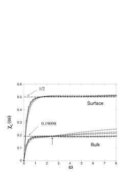
FIG. 6.: Approximants of the bulk and surface magnetization critical exponents vs the order of the moments used to calculate them. The different symbols correspond to different sizes from 5 to 15 ($q=3$, $r=4$).

An interesting consequence of these observations is that one could calculate surface or bulk exponents from an arbitrary value of $\omega$. From the point of view of the finite size scaling analysis we consider values of $\omega$ where the dependence on the system size $L$ is the smallest.

For the data referring to the bulk exponent and shown in the figure we see that around $\omega=2.5$ (this point is indicated by a thick arrow in the figure) finite size effects are very small, all $\chi_{L}(\omega)$ seem to intersect into a single value; for which we estimate $x_{b}=0.1905(5)$ in excellent agreement with the magnetic exponent obtained by Fisher $(3-\sqrt{5})/4\approx 0.19098\ldots$ and also indicated by a thick dashed line in the figure.

TABLE IV.: Calculated bulk exponent from generalized scaling of the moments.

$Q=2$, $r=2$	$Q=2$, $r=8$	$Q=3$, $r=4$	$Q=6$, $r=1.5$
0.189(3)	0.196(3)	0.1910(5)	0.190(2)

Table IV collects the values of bulk exponents calculated with this method. For all cases studied we find a value of $\omega$ for which $\chi_{L}(\omega)$ depends only very weakly on $L$; if the intersection of the $\chi_{L}(\omega)$ for different $L$ is sharp (as in the example shown in Fig. 6) one arrives to a very good estimate of the exponent.

We should also stress that, as the system size enters in Eq. (14) together with $\omega$ in the form of a scaling variable $(1+\omega)\sqrt{L}$. This suggests that higher moments of the magnetizations should show weaker finite size corrections, as increasing $\omega$ has the same effect of enlarging the system size. This is only partially true as Eq. (14) describes only the leading scaling behavior in $1/L$, and it does not include further corrections to scaling terms.

V Correlation functions

In this Section, we deal with the dynamical properties of the random Potts chain. We thus focus here on correlation functions in the temporal direction, which are defined, in the quantum formalism, by:

$$[G_{\sigma\sigma}(t)]_{\rm av}=\left[{\left\langle 0\right|\delta_{\sigma_{i},0}\ e^{-{\cal H}t}\delta_{\sigma_{i},0}\left|0\right\rangle\over\left\langle 0\right|\ e^{-{\cal H}t}\left|0\right\rangle}\right]_{\rm av},$$ (15)

where $\left|0\right\rangle$ denotes the ground state. Fisher’s renormalization group does not provide any information about this quantity. However, Iglói and Rieger by means of scaling arguments derived the following asymptotic behavior:

$$[G_{\sigma\sigma}(t)]_{\rm av}\sim(\ln t)^{-2x_{b}}.$$ (16)

This asymptotic decay of the correlation functions is unusually slow with respect to usual power-law behavior expected at criticality. This can be understood more easily in the classical version of the model and it is due to the fact that disorder along the transfer direction is strongly correlated [32] (layered disorder) and consequently the model displays anisotropic critical behavior. It means that at the critical point, distances measured in space and time directions are connected through power laws involving the dynamical exponent $z$: $t\sim l^{z}$. The homogeneity assumption for the correlation functions thus becomes

$$[G_{\sigma\sigma}(l,t)]_{\rm av}=b^{-2x_{b}}G(l/b,t/b^{z}),$$ (17)

where $b$ is a rescaling factor. The choice $b=t^{1/z}$ thus leads to the usual power-law decay

$$[G_{\sigma\sigma}(l,t)]_{\rm av}\sim t^{-2x_{b}/z}g(l/t^{1/z}),$$ (18)

while in the case of infinite anisotropy ($z\to\infty$) one should set $b=\ln t$ and Eq. (16) follows.

In the classical formulation of the problem followed in this paper, the dynamical correlation function is defined by:

$$[G_{\sigma\sigma}(n)]_{\rm av}=\left[\frac{\langle v_{0}|\delta_{\sigma_{i},0}T^{n}\delta_{\sigma_{i},0}|v_{0}\rangle}{\lambda_{0}^{n}}\right]_{\rm av},$$ (19)

where $\lambda_{0}$ and $|v_{0}\rangle$ are the largest eigenvalue and the corresponding eigenvector of the transfer matrix $T$. For the calculation, we used free boundary conditions on both edges (the magnetization defined by Eq. (4) is thus zero in the whole strip) and we restricted ourselves to the spin in the middle of the system. Since large strip widths are needed in order to avoid finite size effects, average are now performed with $\simeq 25000$ different samples.

FIG. 7.: Dynamical spin-spin correlation functions for the RTIC ($q=2$) at $r=4$ for several strip widths. The number of samples is 25000 for $L=18$ and 24000 for $L=32$ and 48.

Figure 7 shows the correlation function calculated by DMRG techniques following Eq. (19) for $q=2$ and $r=4$. We plot the logarithm of the correlation function vs. the double logarithm of the distance along the time direction (called $n$ in Fig. 1); the dashed line is the asymptotic slope predicted by Eq. (16), where we have used Fisher’s exponent given in Eq. (7). This asymptotic behavior seems to be in agreement with our numerical data for the largest system size analyzed ($L=48$) for which we took $m=16$ and $24000$ disorder realizations.

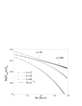
FIG. 8.: Dynamical spin-spin correlation functions for the $q=3$ Potts chain at $r=4$ for several strip widths. The number of samples is 30000 for $L=18$ and 26000 for $L=40$.

Figure 8 shows the analogous plot of the time correlation function for $q=3$ and $r=4$. Again for the largest system size investigated ($L=40$) one notices good agreement with the expected asymptotic limit shown as a thick dashed line. Differently from Fig. 7 we notice here a crossing of the curves representing correlation functions for $L=18$ and $L=40$. This is we believe an effect of the DMRG approach which does not correctly describe the short distance correlation functions, since it does not reproduce the full transfer matrix spectrum. In the other hand, when the number of transfer matrix products becomes large in Eq. (19) the correlation function is determined by the extremal part of the spectrum of $T$, which is believed to be well-reproduced by DMRG methods. Therefore we believe that the crossing of Fig. 8 is due to the limits of the DMRG approximation, while results at larger $n$ should be more accurate.

In conclusion the analysis of the time correlation function for $q=2$ and $q=3$ also indicates that the universal dynamical properties of the disordered quantum Potts chain are independent of $q$.

VI Conclusions

We have provided numerical evidences supporting the conclusions of Senthil and Majumdar [16] concerning the existence of a unique universality class for all finite value of the $q$-state Potts model perturbed by a correlated disorder. For this purpose, we have measured the bulk and surface critical exponents and found values fully compatible with those exactly calculated by Fisher for the RTIC. We point out that a careful numerical study of the critical properties of disordered quantum chains requires an accurate average over randomness, since the most important source of error is due to the disorder average. This effect becomes essential in some circumstances, possibly leading to wrong exponents, and may even dominate other contributions like finite-size effects. For that reason, we generated all the disorder realizations for chains of relatively small lengths, using the fact that the finite-size corrections turned out to be quite small (even compared to their importance in the corresponding pure models). Furthermore, we have checked the expression of the probability distribution by an analysis of its moments: Since the disorder average was exact up to the accuracy of the DMRG method, this computation was allowed even for large moments. The success of this approach is largely due the occurrence of an optimal moment for which the finite-size corrections appear to be extremely weak. The method looks promising for further applications to disordered systems. Finally, we have also compared the expression of the dynamical correlation function with that of the RTIC.

Another interesting feature is the illustration, after the work of Aizenman and Wehr,[7] that correlated disorder induces a second-order phase transition in the $q-$state Potts model with $q>4$. The universality class is however very robust, in contradistinction with the homogeneous two-dimensional disordered fixed point where the magnetic exponents continuously vary with $q$.

- [1] A.B. Harris, J. Phys. C 7, 1671 (1974).
- [2] V.S. Dotsenko, Physics-Uspekhi 38, 457 (1995).
- [3] B.N. Shalaev, Phys. Rep. 237, 129 (1994).
- [4] W. Selke, L.N. Shchur and A.L. Talapov, in Annual Reviews of Computational Physics, edited by D. Stauffer (World Scientific, Singapore, 1994), Vol 1 p. 17.
- [5] Y. Imry and M. Wortis, Phys. Rev. B 19, 3580 (1979).
- [6] K. Hui and A.N. Berker, Phys. Rev. Lett. 62, 2507 (1989).
- [7] M. Aizenman and J. Wehr, Phys. Rev. Lett. 62, 2503 (1989).
- [8] J.L. Cardy and J.L. Jacobsen, Phys. Rev. Lett. 79, 4063 (1997).
- [9] J.L. Jacobsen and J.L. Cardy, Nucl. Phys. B 515, 701 (1998).
- [10] M. Picco, e-print cond-mat/9802092.
- [11] C. Chatelain and B. Berche, Phys. Rev. Lett. 80, 1670 (1998).
- [12] D.S. Fisher, Phys. Rev. Lett. 69, 534 (1992).
- [13] A.P. Young and H. Rieger, Phys. Rev. B 53, 8486 (1996).
- [14] A. Juozapavic̆ius, S. Caprara and A. Rosengren, Phys. Rev. B 56, 11097 (1997).
- [15] H. Rieger and N. Kawashima, e-print cond-mat/9802104.
- [16] T. Senthil and S.N. Majumdar, Phys. Rev. Lett. 76, 3001 (1996).
- [17] B.M. McCoy and T.T. Wu Phys. Rev.176, 631 (1968); B.M. McCoy and T.T. Wu, Phys. Rev.188, 982 (1969); B.M. McCoy, Phys. Rev. 188, 1014 (1969).
- [18] J.B. Kogut, Rev. Mod. Phys. 51, 659 (1979).
- [19] S. R. White, Phys. Rev. Lett.69, 2863 (1992); Phys. Rev. B48, 10345 (1993).
- [20] I. Peschel, X. Wang, M. Kaulke and K. Hallberg (eds.): Density Matrix Renormalization: A New Numerical Method in Physics, Springer, 1999.
- [21] T. Nishino, J. Phys. Soc. Jpn. 64, 3598 (1995).
- [22] S. Wiseman and E. Domany, Phys. Rev. E 51, 3074 (1995).
- [23] N.V. Prokof’ev and B.V. Svistunov, Phys. Rev. Lett. 80, 4355 (1998).
- [24] Similar remarks can be found in S. Rapsch, U. Schollwöck, and W. Zwenger, e-print cond-mat/9901080.
- [25] A. Aharony and A.B. Harris, Phys. Rev. Lett. 77, 3700 (1996).
- [26] S. Wiseman and E. Domany, Phys. Rev. Lett. 81, 22 (1998).
- [27] B. Derrida, Phys. Rep. 29, 103 (1984).
- [28] E. Carlon and F. Iglói, Phys. Rev. B 57, 7877 (1998).
- [29] We followed a different approach than in Ref. [14], where a bulk magnetic field was added to induce a finite magnetization.
- [30] M. Henkel and G. Schütz, J. Phys. A: Math. Gen. 21, 2617 (1988).
- [31] F. Iglói and E. Carlon, Phys. Rev. B 59, 3783 (1999).
- [32] F. Iglói and H. Rieger, Phys. Rev. B 57, 11404 (1998).
- [33] C. Chatelain and B. Berche, Phys. Rev. E 58, R6899 (1998).
- [34] T.W. Burkhardt and T. Xue, Phys. Rev. Lett. 66, 895 (1991).
- [35] M. Henkel, Int. J. Mod. Phys. C3, 1011 (1992).
- [36] M. De Menech, A.L. Stella, and C. Tebaldi, Phys. Rev. E 58, R2677 (1998).
- [37] C. Tebaldi, M. De Menech, and A.L. Stella, e-print cond-mat/9903270.
- [38] With another definition, namely , one would expect in case of self-averaging a unique exponent for all values of , i.e. all the moments would scale like the average.