Orbital polarons in the metal-insulator transition of manganites

Abstract

The metal-insulator transition in manganites is strongly influenced by the concentration of holes present in the system. Based upon an orbitally degenerate Mott-Hubbard model we analyze two possible localization scenarios to account for this doping dependence: First, we rule out that the transition is initiated by a disorder-order crossover in the orbital sector, showing that its effect on charge itineracy is only small. Second, we introduce the idea of orbital polarons originating from a strong polarization of orbitals in the vicinity of holes. Considering this direct coupling between charge and orbital degree of freedom in addition to lattice effects we are able to explain well the phase diagram of manganites for low and intermediate hole concentrations.

]

I Introduction

The doping dependence of the properties of manganese oxides poses some of the most interesting open problems in the physics of these compounds. First to be noticed is the peculiar asymmetry of the phase diagram that is most pronounced in the charge sector: Regions of high ($x>0.5$) and low ($x<0.5$) concentration of holes are characterized by such contrasting phenomena as charge ordering and metalicity, respectively. In the latter region — which we wish to focus on — the metallic state can be turned into an insulating one by raising the temperature above the Curie temperature $T_{C}$. Introducing the notion of double exchange which associates the relative orientation of localized Mn $t_{2g}$ spins with the mobility of itinerant $e_{g}$ electrons, early work has identified this transition to be controlled by the loss of ferromagnetic order inherent to the metallic state.[1] It is believed that lattice effects are also of crucial importance in this transition. Within the lattice-polaron double-exchange picture,[2, 3] the crossover from metallic to insulating behavior is controlled by the ratio of polaron binding energy $E_{b}$ to the kinetic energy $E_{\text{kin}}$ of charge carriers:

$$\lambda=\frac{E_{b}}{E_{\text{kin}}}.$$ (1)

When forming a bound state with the lattice, charge carriers loose part of their kinetic energy. Hence, polarons are stable only if this loss in energy is more than compensated by the gain in binding energy, i.e., if $\lambda>1$. In a double-exchange system, this critical coupling strength may be reached by raising the temperature — the double-exchange mechanism then acts to reduce the kinetic energy and hence to increase $\lambda$. Spin disorder and spin-polaron effects further enhance the carrier localization above $T_{C}$.[4] The doping dependence of the metal-insulator transition, however, is not fully captured in this picture. Namely the complete breakdown of metalicity at hole concentrations below $x_{\text{crit}}\approx 0.15$ - $0.2$ that occurs despite the fact that ferromagnetism is fully sustained remains an open problem which we address in this paper.

The effective coupling constant $\lambda$ in Eq. (1) has originally been introduced for non-interacting electrons. The itinerant $e_{g}$ electrons in manganites, on the other hand, are subject to strong on-site repulsions which necessitates to accommodate the definition of $\lambda$. According to numerical studies, [5] the basic physics underlying Eq. (1) remains valid even in correlated systems: As in the free-electron case, the metal-insulator transition is controlled by the competition between the polaron binding energy and the kinetic energy of charge carriers. Nevertheless, correlation effects might renormalize these two relevant energy scales, presumably introducing a doping dependence. In fact, the Gutzwiller bandwidth of correlated electrons scales with the concentration of doped holes; one could therefore be inclined to set $E_{\text{kin}}\propto xt$, where $t$ denotes the hopping amplitude. But this approach reaches too short: The Gutzwiller picture describes only the average kinetic energy of the system. In contrast, the relevant quantity for localizing the holes doped into a Mott-Hubbard system is the characteristic energy scale of charge fluctuations which remains $\propto t$.[6] Pictorially this quantity corresponds to the kinetic energy of a single hole. We thus conclude that a more thorough treatment of correlation effects is needed in order to explain the peculiar doping dependence of the metal-insulator transition in manganites.

In this paper we analyze two mechanisms that could drive the localization of charge carriers at small hole concentrations $x$. First we explore the possibility of the metal-insulator transition to be controlled by a disorder-order crossover in the $e_{g}$-orbital sector. The idea is the following: Orbital fluctuations are induced by the motion of holes and hence possess an energy scale $\propto xt$. At large $x$, orbitals fluctuate strongly and inter-site orbital correlations are weak. As the concentration of holes is reduced, fluctuations slow down until a critical value of $x$ has been reached — promoted by Jahn-Teller and superexchange coupling, an orbital-lattice ordered state now evolves. We analyze the extent to which this transition in the orbital-lattice sector affects the itineracy of holes. Finding almost similar values for the kinetic energy of doped holes in orbitally ordered and disordered states we are lead to conclude that the development of orbital-lattice order is not sufficient to trigger the localization process. Next we turn to analyze a second scenario of the metal-insulator transition for which we introduce the concept of orbital polarons. Similar to spin polarons in correlated spin systems, orbital polarons are a natural consequence of strong electron correlations and the double degeneracy of on-site levels — in manganites the latter follows from the degeneracy of $e_{g}$ orbitals. We argue that holes polarize the orbital state of $e_{g}$ electrons on neighboring sites: A splitting of orbital levels is evoked by a displacement of oxygen ions and also by the Coulomb force exerted by the positively charged holes. Being comparable in magnitude to the kinetic energy of holes, the orbital-hole binding energy can be large enough for holes and surrounding orbitals to form a bound state. The important point is that the stability of these orbital polarons competes not only against the kinetic energy of holes but also against the fluctuation rate $\propto xt$ of orbitals: The faster the latter fluctuate, the less favorable it is to form a bound state in which orbitals have to give up part of their fluctuation energy. Combining this new orbital-polaron picture with that of conventional lattice polarons we are able to explain well the phase diagram of manganites at low and intermediate doping levels.

II Orbital Disorder-Order Transition

In this section we analyze the impact of a disorder-order transition in the orbital-lattice sector onto the itineracy of holes. Our motivation is that a sudden freezing out of orbital fluctuations below a critical doping concentration could significantly impede the motion of holes, hence initiating the metal-insulator transition. By comparing the bandwidth of holes both in orbitally ordered and disordered states, we are able to refute this idea: The orbital sector is shown to have only little influence onto the charge mobility in manganites.

A Disordered State

We begin by investigating the bandwidth of holes in a strongly fluctuating, orbitally disordered state. Our starting point is the $t$-$J$ model of double-degenerate $e_{g}$ electrons which, via Hund’s coupling, interact ferromagnetically with an array of localized $S=3/2$ core spins. The model accounts for the presence of strong on-site repulsions that forbids more than one $e_{g}$ electron to occupy the same Mn site as well as for the double-degeneracy of $e_{g}$ levels. At low temperatures and intermediate doping levels, the double-exchange mechanism induces a parallel alignment of spins. Treating deviations from this ferromagnetic ground state only on a mean-field level as is discussed below, the core spins can be discarded and the spin indices of $e_{g}$ electrons may be dropped; the $t$-$J$ Hamiltonian then becomes[7, 8]

$$H_{tJ}=-\sum_{\langle ij\rangle_{\gamma}}\left(t^{\alpha\beta}_{\gamma}\hat{c}^{\dagger}_{i\alpha}\hat{c}_{j\beta}+\text{H.c.}\right)+\frac{2J}{z}\sum_{\langle ij\rangle_{\gamma}}\tau^{\gamma}_{i}\tau^{\gamma}_{j},$$ (2)

with $z=6$. Nearest-neighbor bonds along spatial directions $\gamma\in\{x,y,z\}$ are denoted by $\langle ij\rangle_{\gamma}$. We use constrained operators $\hat{c}^{\dagger}_{i\alpha}=c^{\dagger}_{i\alpha}\left(1-n_{i}\right)$ which create an $e_{g}$ electron at site $i$ in orbital $\alpha$ only under the condition that the site is empty. The first term in Eq. (2) describes the inter-site transfer of constrained $e_{g}$ electrons. The transfer amplitude depends upon the orientation of orbitals at a given bond as is reflected by the transfer matrices

$\displaystyle t_{x/y}^{\alpha\beta}=t\left(\begin{array}[]{cc}1/4&\mp\sqrt{3}/4\\ \mp\sqrt{3}/4&3/4\end{array}\right),\quad t_{z}^{\alpha\beta}=t\left(\begin{array}[]{cc}1&0\\ 0&0\end{array}\right);$

a representation with respect to the orbital basis $\alpha\in\{|3z^{2}-r^{2}\rangle,|x^{2}-y^{2}\rangle\}$ has been chosen here. Due to its non-diagonal structure, orbital quantum numbers are not conserved by Hamiltonian (2) – inter-site transfer processes induce fluctuations in the orbital sector. The second term in Eq. (2) accounts for processes involving the virtual occupation of sites by two $e_{g}$ electrons. This superexchange mechanism establishes an inter-site coupling between orbital pseudospins of overall strength $J=zt^{2}/U$, where $U$ is the on-site repulsion between spin-parallel $e_{g}$ electrons. The pseudospin operators are

$$\tau^{x/y}_{i}=-\frac{1}{4}(\sigma^{z}\pm\sqrt{3}\sigma^{x}),\quad\tau^{z}_{i}=\frac{1}{2}\sigma^{z},$$ (3)

with Pauli matrices $\sigma^{x/z}_{i}$ acting on the orbital subspace. Jahn-Teller phonons mediate an additional interaction between orbital pseudospins which is of the exact same form as the superexchange term. The numerical value of $J$ has to be chosen such as to comprise both effects. We finally note that deviations from the ferromagnetic ground state underlying Hamiltonian (2) are treated within conventional double-exchange theory. The transfer amplitude $t$ then depends on the normalized magnetization $m$ via[2, 9]

$$t=t_{0}\sqrt{(1+m^{2})/2},$$ (4)

where $t_{0}$ denotes the hopping amplitude between spin-parallel Mn sites.

To observe the strongly correlated nature of $e_{g}$ electrons, it is convenient to introduce separate particles for charge and orbital degrees of freedom.[10] The metallic phase of manganites can be well described within an orbital-liquid picture that accounts for orbital fluctuations by employing a slave-boson representation of electron operators:[8, 11]

$\displaystyle c^{\dagger}_{i\alpha}=f^{\dagger}_{i\alpha}b_{i}.$

Here orbital pseudospin is carried by fermionic orbitons $f_{i\alpha}$ and charge by bosonic holons $b_{i}$. Introducing mean-field parameters $\chi=t^{-1}\sum_{\alpha\beta}t^{\alpha\beta}_{\gamma}\langle f^{\dagger}_{i\alpha}f_{i\beta}\rangle$ and $x=\langle b^{\dagger}_{i}b_{j}\rangle$, where $x$ is the concentration of holes and $\chi\approx\frac{1}{2}$, the two types of quasiparticles can be decoupled:

$$H_{\text{orb}} = -\left(x+\frac{2\chi J}{zt}\right)\sum_{\langle ij\rangle_{\gamma}}t^{\alpha\beta}_{\gamma}\left(f^{\dagger}_{i\alpha}f_{j\beta}+\text{H.c.}\right),$$ (5)

$$H_{\text{hl}} = -\chi t\sum_{\langle ij\rangle}\left(b^{\dagger}_{i}b_{j}+\text{H.c.}\right).$$ (6)

Diagonalizing the above expressions in the momentum representation one obtains

$\displaystyle H_{\text{orb}}=\sum_{\mathchoice{{\hbox{\boldmath$\displaystyle k$}}}{{\hbox{\boldmath$\textstyle k$}}}{{\hbox{\boldmath$\scriptstyle k$}}}{{\hbox{\boldmath$\scriptscriptstyle k$}}}\nu}\xi^{\nu}_{\mathchoice{{\hbox{\boldmath$\displaystyle k$}}}{{\hbox{\boldmath$\textstyle k$}}}{{\hbox{\boldmath$\scriptstyle k$}}}{{\hbox{\boldmath$\scriptscriptstyle k$}}}}f^{\dagger}_{\mathchoice{{\hbox{\boldmath$\displaystyle k$}}}{{\hbox{\boldmath$\textstyle k$}}}{{\hbox{\boldmath$\scriptstyle k$}}}{{\hbox{\boldmath$\scriptscriptstyle k$}}}\nu}f_{\mathchoice{{\hbox{\boldmath$\displaystyle k$}}}{{\hbox{\boldmath$\textstyle k$}}}{{\hbox{\boldmath$\scriptstyle k$}}}{{\hbox{\boldmath$\scriptscriptstyle k$}}}\nu},\quad H_{\text{hl}}=\sum_{\mathchoice{{\hbox{\boldmath$\displaystyle k$}}}{{\hbox{\boldmath$\textstyle k$}}}{{\hbox{\boldmath$\scriptstyle k$}}}{{\hbox{\boldmath$\scriptscriptstyle k$}}}}\omega_{\mathchoice{{\hbox{\boldmath$\displaystyle k$}}}{{\hbox{\boldmath$\textstyle k$}}}{{\hbox{\boldmath$\scriptstyle k$}}}{{\hbox{\boldmath$\scriptscriptstyle k$}}}}b^{\dagger}_{\mathchoice{{\hbox{\boldmath$\displaystyle k$}}}{{\hbox{\boldmath$\textstyle k$}}}{{\hbox{\boldmath$\scriptstyle k$}}}{{\hbox{\boldmath$\scriptscriptstyle k$}}}}b_{\mathchoice{{\hbox{\boldmath$\displaystyle k$}}}{{\hbox{\boldmath$\textstyle k$}}}{{\hbox{\boldmath$\scriptstyle k$}}}{{\hbox{\boldmath$\scriptscriptstyle k$}}}},$

with index $\nu=\pm$ and dispersion functions

$$\xi^{\pm}_{\mathchoice{{\hbox{\boldmath$\displaystyle k$}}}{{\hbox{\boldmath$\textstyle k$}}}{{\hbox{\boldmath$\scriptstyle k$}}}{{\hbox{\boldmath$\scriptscriptstyle k$}}}} = (xt+\frac{2\chi J}{z})\Big{[}-\epsilon_{0}(\mathchoice{{\hbox{\boldmath$\displaystyle k$}}}{{\hbox{\boldmath$\textstyle k$}}}{{\hbox{\boldmath$\scriptstyle k$}}}{{\hbox{\boldmath$\scriptscriptstyle k$}}})\pm\sqrt{\epsilon_{1}^{2}(\mathchoice{{\hbox{\boldmath$\displaystyle k$}}}{{\hbox{\boldmath$\textstyle k$}}}{{\hbox{\boldmath$\scriptstyle k$}}}{{\hbox{\boldmath$\scriptscriptstyle k$}}})+\epsilon_{2}^{2}(\mathchoice{{\hbox{\boldmath$\displaystyle k$}}}{{\hbox{\boldmath$\textstyle k$}}}{{\hbox{\boldmath$\scriptstyle k$}}}{{\hbox{\boldmath$\scriptscriptstyle k$}}})}\Big{]},$$ (7)

$$\omega_{\mathchoice{{\hbox{\boldmath$\displaystyle k$}}}{{\hbox{\boldmath$\textstyle k$}}}{{\hbox{\boldmath$\scriptstyle k$}}}{{\hbox{\boldmath$\scriptscriptstyle k$}}}} = 6\chi t\Big{[}1-\frac{1}{3}\epsilon_{0}(\mathchoice{{\hbox{\boldmath$\displaystyle k$}}}{{\hbox{\boldmath$\textstyle k$}}}{{\hbox{\boldmath$\scriptstyle k$}}}{{\hbox{\boldmath$\scriptscriptstyle k$}}})\Big{]},$$ (8)

where $\epsilon_{0}(\mathchoice{{\hbox{\boldmath$\displaystyle k$}}}{{\hbox{\boldmath$\textstyle k$}}}{{\hbox{\boldmath$\scriptstyle k$}}}{{\hbox{\boldmath$\scriptscriptstyle k$}}})=c_{x}+c_{y}+c_{z}$, $\epsilon_{1}(\mathchoice{{\hbox{\boldmath$\displaystyle k$}}}{{\hbox{\boldmath$\textstyle k$}}}{{\hbox{\boldmath$\scriptstyle k$}}}{{\hbox{\boldmath$\scriptscriptstyle k$}}})=(c_{x}+c_{y})/2-c_{z}$, $\epsilon_{2}(\mathchoice{{\hbox{\boldmath$\displaystyle k$}}}{{\hbox{\boldmath$\textstyle k$}}}{{\hbox{\boldmath$\scriptstyle k$}}}{{\hbox{\boldmath$\scriptscriptstyle k$}}})=\sqrt{3}(c_{x}-c_{y})/2$ with $c_{\gamma}=\cos k_{\gamma}$. The essence of this slaved-particle mean-field treatment is that orbital and charge fluctuations are assigned different energy scales. This is reflected by the bandwidths of orbiton and holon quasiparticles, respectively:

$$W_{\text{orb}} = 6xt+J,$$ (9)

$$W_{\text{hl}} = 6t.$$ (10)

The former quantity $W_{\text{orb}}$ sets the energy scale of orbital fluctuations — the terms proportional to $xt$ and $J$ describe fluctuations induced by the motion of holes and by the coupling between pseudospins, respectively. The latter quantity $W_{\text{hl}}$ finally defines the itineracy of holes in the orbital-liquid state. The variation of the holon bandwidth with the onset of orbital order is in the focus of our interest in the remainder of this section.

B Instability Toward Orbital Order

The above treatment of orbital and charge fluctuations is based upon the notion of a strongly fluctuating orbital state that is far from any instability towards orbital order. In real systems such instabilities do exist: Jahn-Teller phonons and superexchange processes mediate a coupling between orbitals on neighboring sites which introduces a bias towards orbital-lattice ordering. Competing against the energy scale of orbital fluctuations $\propto xt$, order in the orbital sector is expected to evolve below a critical doping concentration $x_{\text{crit}}$. We investigate this instability of the orbital-liquid state by introducing the inter-site coupling term

$$H_{J}=-\frac{2J}{z}\sum_{\langle ij\rangle_{\gamma}}\tau_{i}^{\Theta}\tau_{j}^{\Theta}\,e^{iQ_{\gamma}},$$ (11)

with $z=6$ and $\tau_{i}=(\sin\Theta\sigma^{x}_{i}+\cos\Theta\sigma^{z}_{i})/2$ acting on the orbital subspace. We note that Eq. (11) is a simplification of the superexchange coupling term in Hamiltonian (2) — internal frustration makes the latter difficult to handle. For $\Theta=\pi/2$ and $\mathchoice{{\hbox{\boldmath$\displaystyle Q$}}}{{\hbox{\boldmath$\textstyle Q$}}}{{\hbox{\boldmath$\scriptstyle Q$}}}{{\hbox{\boldmath$\scriptscriptstyle Q$}}}=(\pi,\pi,0)$, the pseudospin interaction in Eq. (11) favors a staggered-type orbital orientation

$$|\Theta\rangle^{\pm}=\left(|3z^{2}-r^{2}\rangle\pm|x^{2}-y^{2}\rangle\right)/\sqrt{2}$$ (12)

within $x$-$y$ planes repeating itself along the $z$ direction; this closely resembles the type of order observed experimentally in LaMnO₃.[12] The breakdown of the orbitally disordered state, i.e., the development of orbital order, is signaled by a singularity in the static orbital susceptibility $\langle\sigma_{\mathchoice{{\hbox{\boldmath$\displaystyle Q$}}}{{\hbox{\boldmath$\textstyle Q$}}}{{\hbox{\boldmath$\scriptstyle Q$}}}{{\hbox{\boldmath$\scriptscriptstyle Q$}}}}^{x}\sigma_{-\mathchoice{{\hbox{\boldmath$\displaystyle Q$}}}{{\hbox{\boldmath$\textstyle Q$}}}{{\hbox{\boldmath$\scriptstyle Q$}}}{{\hbox{\boldmath$\scriptscriptstyle Q$}}}}^{x}\rangle_{\omega=0}$. Employing a random-phase approximation, the latter can be expressed as

$$\langle\sigma^{x}\sigma^{x}\rangle_{\mathchoice{{\hbox{\boldmath$\displaystyle Q$}}}{{\hbox{\boldmath$\textstyle Q$}}}{{\hbox{\boldmath$\scriptstyle Q$}}}{{\hbox{\boldmath$\scriptscriptstyle Q$}}}}=\frac{\langle\sigma^{x}\sigma^{x}\rangle^{0}_{\mathchoice{{\hbox{\boldmath$\displaystyle Q$}}}{{\hbox{\boldmath$\textstyle Q$}}}{{\hbox{\boldmath$\scriptstyle Q$}}}{{\hbox{\boldmath$\scriptscriptstyle Q$}}}}}{1+J_{\mathchoice{{\hbox{\boldmath$\displaystyle Q$}}}{{\hbox{\boldmath$\textstyle Q$}}}{{\hbox{\boldmath$\scriptstyle Q$}}}{{\hbox{\boldmath$\scriptscriptstyle Q$}}}}\langle\sigma^{x}\sigma^{x}\rangle^{0}_{\mathchoice{{\hbox{\boldmath$\displaystyle Q$}}}{{\hbox{\boldmath$\textstyle Q$}}}{{\hbox{\boldmath$\scriptstyle Q$}}}{{\hbox{\boldmath$\scriptscriptstyle Q$}}}}/2},$$ (13)

with vertex function $J_{\mathchoice{{\hbox{\boldmath$\displaystyle q$}}}{{\hbox{\boldmath$\textstyle q$}}}{{\hbox{\boldmath$\scriptstyle q$}}}{{\hbox{\boldmath$\scriptscriptstyle q$}}}}=J\left(\cos q_{x}+\cos q_{y}-\cos q_{z}\right)/3$ and the shorthand notation $\langle\sigma^{x}\sigma^{x}\rangle_{\mathchoice{{\hbox{\boldmath$\displaystyle Q$}}}{{\hbox{\boldmath$\textstyle Q$}}}{{\hbox{\boldmath$\scriptstyle Q$}}}{{\hbox{\boldmath$\scriptscriptstyle Q$}}}}=\langle\sigma_{\mathchoice{{\hbox{\boldmath$\displaystyle Q$}}}{{\hbox{\boldmath$\textstyle Q$}}}{{\hbox{\boldmath$\scriptstyle Q$}}}{{\hbox{\boldmath$\scriptscriptstyle Q$}}}}^{x}\sigma_{-\mathchoice{{\hbox{\boldmath$\displaystyle Q$}}}{{\hbox{\boldmath$\textstyle Q$}}}{{\hbox{\boldmath$\scriptstyle Q$}}}{{\hbox{\boldmath$\scriptscriptstyle Q$}}}}^{x}\rangle_{\omega=0}$. Bare orbital susceptibilities $\langle\ldots\rangle^{0}$ are evaluated using orbiton propagators associated with the mean-field Hamiltonian (5). Numerically solving for the pole in Eq. (13), we find the following expression for the critical doping concentration:

$$x_{\text{crit}}\approx\frac{J}{4t},$$ (14)

which is valid for $x_{\text{crit}}\ll 0.5$. At concentrations below this critical value an orbitally ordered state is to be expected. With $J=0.13$ eV as estimated from the structural phase transition observed in LaMnO₃ at $T=780$ K (Ref. [12]) and $t=0.36$ eV (Ref. [8]) we obtain a critical doping concentration of $x_{\text{crit}}=9\%$. This result indicates that the metallic state of manganites is indeed instable towards orbital-lattice ordering at doping concentrations that are not too far from those at which the system is observed to become insulating.

C Ordered State

Up to this point we have studied the bandwidth of holes in an orbitally disordered state and the instability of the system towards orbital-lattice order. In the following we analyze to which extent the itineracy of holes is affected by this disorder-order transition in the orbital sector. Namely we are interested in the bandwidth of holes moving through an orbitally ordered state; this quantity is then compared to our previous result of Eq. (10) for an orbital liquid. Foremost an important difference between models with orbital pseudospin and conventional spin is to be noticed here: In the latter systems, spin is conserved when electrons hop between sites. This implies that hole motion is constrained in a staggered spin background. In contrast, the transfer Hamiltonian (2) of the orbital model is non-diagonal in orbital pseudospin — an orbital basis in which all three transfer matrices $t_{x}^{\alpha\beta}$, $t_{y}^{\alpha\beta}$, and $t_{z}^{\alpha\beta}$ are of diagonal structure does not exist. This allows holes to move coherently even within an antiferro-type orbital arrangement [see Fig. 1(a)].

FIG. 1.: Coherent (a) and incoherent (b) hole motion in antiferro-type orbital order. Incoherent processes involve the creation of an orbital excitation of energy $J$.

For this reason only a moderate suppression of the hole bandwidth is to be expected in the presence of orbital order. We calculate the bandwidth for the specific type of orbital order introduced in Eq. (12). Starting from the transfer part of Hamiltonian (2) and keeping only the hopping matrix elements that allow for a coherent movement of holes (i.e., projecting out all orbitals which do not comply with the ordered state) we obtain

$$W_{\text{hl}}^{\text{coh}}=4t.$$ (15)

This result indicates a reduction of the holon bandwidth by $\approx 30\%$ as compared to the disordered state [see Eq. (10)]. While not being dramatic, a quenching of the bandwidth by one third should nevertheless be sufficient to induce the localization process, e.g., via the formation of lattice polarons. However, it is important to note that Eq. (15) accounts solely for the coherent motion of holes; incoherent processes involving the creation and subsequent absorption of orbital excitations are neglected [see Fig. 1(b)]. Only if the ordered state is robust, i.e., if it costs a large amount of energy for an electron to occupy an orbital that does not comply with the long-range orbital alignment, these incoherent processes become negligible. This limit does not apply to manganites where the orbital excitation energy is $J<t$ only. Before a conclusion about the role of orbital order in the metal-insulator transition can be drawn, these incoherent processes have to be investigated in more detail.

In the following we study the influence of incoherent processes onto the motion of holes, employing an “orbital wave” approximation: Starting from the assumption that long-range orbital order has developed and that fluctuations around this ordered state are weak, we use a slave-fermion representation of the electron operators in the transfer Hamiltonian (2):

$\displaystyle c^{\dagger}_{i\alpha}=b^{\dagger}_{i\alpha}f_{i}.$

Within this picture, the orbital pseudospin is assigned to bosonic orbitons and charge to fermionic holons. The lattice is then divided into two sublattices which are ascribed different preferred pseudospin directions [see Eq. (12)]:

$$\uparrow \equiv \left(|3z^{2}-r^{2}\rangle+|x^{2}-y^{2}\rangle\right)/\sqrt{2}\quad\text{on sublattice $A$},$$

$$\downarrow \equiv \left(|3z^{2}-r^{2}\rangle-|x^{2}-y^{2}\rangle\right)/\sqrt{2}\quad\text{on sublattice $B$}.$$

In analogy to conventional spin-wave theory, excitations around this ground state can be treated by employing the following mapping of orbiton operators $b_{i\alpha}$ onto “orbital-wave” operators $\beta_{i}$:

$\displaystyle b_{i\uparrow}=\left\{\begin{array}[]{cc}1&\text{sublattice $A$},\\ \beta_{i}&\text{sublattice $B$},\end{array}\right.\quad b_{i\downarrow}=\left\{\begin{array}[]{cc}\beta_{i}&\text{sublattice $A$},\\ 1&\text{sublattice $B$}.\end{array}\right.$

In the momentum representation the transfer Hamiltonian (2) then becomes

$$H_{t}=\sum_{\mathchoice{{\hbox{\boldmath$\displaystyle k$}}}{{\hbox{\boldmath$\textstyle k$}}}{{\hbox{\boldmath$\scriptstyle k$}}}{{\hbox{\boldmath$\scriptscriptstyle k$}}}}\omega_{\mathchoice{{\hbox{\boldmath$\displaystyle k$}}}{{\hbox{\boldmath$\textstyle k$}}}{{\hbox{\boldmath$\scriptstyle k$}}}{{\hbox{\boldmath$\scriptscriptstyle k$}}}}f_{\mathchoice{{\hbox{\boldmath$\displaystyle k$}}}{{\hbox{\boldmath$\textstyle k$}}}{{\hbox{\boldmath$\scriptstyle k$}}}{{\hbox{\boldmath$\scriptscriptstyle k$}}}}^{\dagger}f_{\mathchoice{{\hbox{\boldmath$\displaystyle k$}}}{{\hbox{\boldmath$\textstyle k$}}}{{\hbox{\boldmath$\scriptstyle k$}}}{{\hbox{\boldmath$\scriptscriptstyle k$}}}}+\sum_{\mathchoice{{\hbox{\boldmath$\displaystyle k$}}}{{\hbox{\boldmath$\textstyle k$}}}{{\hbox{\boldmath$\scriptstyle k$}}}{{\hbox{\boldmath$\scriptscriptstyle k$}}}\mathchoice{{\hbox{\boldmath$\displaystyle p$}}}{{\hbox{\boldmath$\textstyle p$}}}{{\hbox{\boldmath$\scriptstyle p$}}}{{\hbox{\boldmath$\scriptscriptstyle p$}}}}\left[\gamma_{\mathchoice{{\hbox{\boldmath$\displaystyle k$}}}{{\hbox{\boldmath$\textstyle k$}}}{{\hbox{\boldmath$\scriptstyle k$}}}{{\hbox{\boldmath$\scriptscriptstyle k$}}}}\beta^{\dagger}_{\mathchoice{{\hbox{\boldmath$\displaystyle p$}}}{{\hbox{\boldmath$\textstyle p$}}}{{\hbox{\boldmath$\scriptstyle p$}}}{{\hbox{\boldmath$\scriptscriptstyle p$}}}}+\gamma_{\mathchoice{{\hbox{\boldmath$\displaystyle k$}}}{{\hbox{\boldmath$\textstyle k$}}}{{\hbox{\boldmath$\scriptstyle k$}}}{{\hbox{\boldmath$\scriptscriptstyle k$}}}+\mathchoice{{\hbox{\boldmath$\displaystyle p$}}}{{\hbox{\boldmath$\textstyle p$}}}{{\hbox{\boldmath$\scriptstyle p$}}}{{\hbox{\boldmath$\scriptscriptstyle p$}}}}\beta_{-\mathchoice{{\hbox{\boldmath$\displaystyle p$}}}{{\hbox{\boldmath$\textstyle p$}}}{{\hbox{\boldmath$\scriptstyle p$}}}{{\hbox{\boldmath$\scriptscriptstyle p$}}}}\right]f_{\mathchoice{{\hbox{\boldmath$\displaystyle k$}}}{{\hbox{\boldmath$\textstyle k$}}}{{\hbox{\boldmath$\scriptstyle k$}}}{{\hbox{\boldmath$\scriptscriptstyle k$}}}}^{\dagger}f_{\mathchoice{{\hbox{\boldmath$\displaystyle k$}}}{{\hbox{\boldmath$\textstyle k$}}}{{\hbox{\boldmath$\scriptstyle k$}}}{{\hbox{\boldmath$\scriptscriptstyle k$}}}+\mathchoice{{\hbox{\boldmath$\displaystyle p$}}}{{\hbox{\boldmath$\textstyle p$}}}{{\hbox{\boldmath$\scriptstyle p$}}}{{\hbox{\boldmath$\scriptscriptstyle p$}}}}.$$ (16)

Here $\omega_{\mathchoice{{\hbox{\boldmath$\displaystyle k$}}}{{\hbox{\boldmath$\textstyle k$}}}{{\hbox{\boldmath$\scriptstyle k$}}}{{\hbox{\boldmath$\scriptscriptstyle k$}}}}=-t(c_{x}+c_{y}-2c_{z})/2$ and $\gamma_{\mathchoice{{\hbox{\boldmath$\displaystyle k$}}}{{\hbox{\boldmath$\textstyle k$}}}{{\hbox{\boldmath$\scriptstyle k$}}}{{\hbox{\boldmath$\scriptscriptstyle k$}}}}=t[(2-\sqrt{3})c_{x}+(2+\sqrt{3})c_{y}+2c_{z}]/2$ with $c_{\gamma}=\cos k_{\gamma}$. The first term in Eq. (16) describes the coherent motion of holes within a band of width $W_{\text{hl}}^{\text{coh}}=4t$. The second term describes the interaction of holes with excitations of the orbital background. The dynamics of the latter is controlled by the inter-site coupling Hamiltonian (11) which in the momentum representation becomes

$$H_{J}=J\sum_{\mathchoice{{\hbox{\boldmath$\displaystyle k$}}}{{\hbox{\boldmath$\textstyle k$}}}{{\hbox{\boldmath$\scriptstyle k$}}}{{\hbox{\boldmath$\scriptscriptstyle k$}}}}\beta^{\dagger}_{\mathchoice{{\hbox{\boldmath$\displaystyle k$}}}{{\hbox{\boldmath$\textstyle k$}}}{{\hbox{\boldmath$\scriptstyle k$}}}{{\hbox{\boldmath$\scriptscriptstyle k$}}}}\beta_{\mathchoice{{\hbox{\boldmath$\displaystyle k$}}}{{\hbox{\boldmath$\textstyle k$}}}{{\hbox{\boldmath$\scriptstyle k$}}}{{\hbox{\boldmath$\scriptscriptstyle k$}}}}.$$ (17)

Hamiltonian (17) describes dispersionless, non-propagating orbital excitations of energy $J$. The local nature of orbital excitations follows from the absence of frustration effects in the inter-site orbital coupling term (11).

The interaction of holes with orbital degrees of freedom changes the character of the hole motion: Scattering on orbital excitations leads to a suppression of the coherent quasiparticle weight and a simultaneous widening of the holon band. In analogy to studies of spin systems,[13, 14] we analyze these effects by employing a self-consistent Born approximation for the self energy of holes — within this method all non-crossing diagrams of the self energy are summed up to infinite order while crossing diagrams are neglected. Restricting ourselves to the case of a single hole moving at the bottom of the band, we obtain the following expression for the holon self energy (see Fig. 2):

FIG. 2.: Born approximation of the holon self energy: The double line denotes the “dressed” holon propagator with self-energy contributions, the dashed line represents the “orbital-wave” Green’s function.

$$\Sigma(i\omega)=t^{2}\sum_{\mathchoice{{\hbox{\boldmath$\displaystyle p$}}}{{\hbox{\boldmath$\textstyle p$}}}{{\hbox{\boldmath$\scriptstyle p$}}}{{\hbox{\boldmath$\scriptscriptstyle p$}}}}\gamma^{2}_{\mathchoice{{\hbox{\boldmath$\displaystyle p$}}}{{\hbox{\boldmath$\textstyle p$}}}{{\hbox{\boldmath$\scriptstyle p$}}}{{\hbox{\boldmath$\scriptscriptstyle p$}}}}\;G(i\omega-J,\mathchoice{{\hbox{\boldmath$\displaystyle p$}}}{{\hbox{\boldmath$\textstyle p$}}}{{\hbox{\boldmath$\scriptstyle p$}}}{{\hbox{\boldmath$\scriptscriptstyle p$}}}).$$ (18)

The Matsubara frequencies are defined as $i\omega=i(2n+1)\pi T$, where $T$ denotes temperature and $n$ an integer number.

Our first aim is to study the loss of coherency in the hole motion. This can be done by employing a dominant-pole approximation:[13] We split the holon propagator in Eq. (18) into its coherent and incoherent parts,

$$G(i\omega,\mathchoice{{\hbox{\boldmath$\displaystyle k$}}}{{\hbox{\boldmath$\textstyle k$}}}{{\hbox{\boldmath$\scriptstyle k$}}}{{\hbox{\boldmath$\scriptscriptstyle k$}}})=\frac{a_{\mathchoice{{\hbox{\boldmath$\displaystyle k$}}}{{\hbox{\boldmath$\textstyle k$}}}{{\hbox{\boldmath$\scriptstyle k$}}}{{\hbox{\boldmath$\scriptscriptstyle k$}}}}}{i\omega-\tilde{\omega}_{\mathchoice{{\hbox{\boldmath$\displaystyle k$}}}{{\hbox{\boldmath$\textstyle k$}}}{{\hbox{\boldmath$\scriptstyle k$}}}{{\hbox{\boldmath$\scriptscriptstyle k$}}}}}+G^{\text{inc}}(i\omega,\mathchoice{{\hbox{\boldmath$\displaystyle k$}}}{{\hbox{\boldmath$\textstyle k$}}}{{\hbox{\boldmath$\scriptstyle k$}}}{{\hbox{\boldmath$\scriptscriptstyle k$}}}),$$ (19)

where $a_{\mathchoice{{\hbox{\boldmath$\displaystyle k$}}}{{\hbox{\boldmath$\textstyle k$}}}{{\hbox{\boldmath$\scriptstyle k$}}}{{\hbox{\boldmath$\scriptscriptstyle k$}}}}$ denotes the quasiparticle weight and $\tilde{\omega}_{\mathchoice{{\hbox{\boldmath$\displaystyle k$}}}{{\hbox{\boldmath$\textstyle k$}}}{{\hbox{\boldmath$\scriptstyle k$}}}{{\hbox{\boldmath$\scriptscriptstyle k$}}}}$ the not-yet-known renormalized holon dispersion. Keeping only the coherent part and using $a_{\mathchoice{{\hbox{\boldmath$\displaystyle k$}}}{{\hbox{\boldmath$\textstyle k$}}}{{\hbox{\boldmath$\scriptstyle k$}}}{{\hbox{\boldmath$\scriptscriptstyle k$}}}}=[1-(\partial/\partial\omega)\Sigma^{\prime}(\omega)]^{-1}$ with $\Sigma^{\prime}(\omega)=\text{Re}[\Sigma(i\omega\rightarrow\omega+i0^{+})]$, the following recursion relation for the quasiparticle weight is obtained:

$$a_{\bar{\mathchoice{{\hbox{\boldmath$\displaystyle q$}}}{{\hbox{\boldmath$\textstyle q$}}}{{\hbox{\boldmath$\scriptstyle q$}}}{{\hbox{\boldmath$\scriptscriptstyle q$}}}}}=\left[1+t^{2}\sum_{\mathchoice{{\hbox{\boldmath$\displaystyle p$}}}{{\hbox{\boldmath$\textstyle p$}}}{{\hbox{\boldmath$\scriptstyle p$}}}{{\hbox{\boldmath$\scriptscriptstyle p$}}}}\gamma_{\mathchoice{{\hbox{\boldmath$\displaystyle p$}}}{{\hbox{\boldmath$\textstyle p$}}}{{\hbox{\boldmath$\scriptstyle p$}}}{{\hbox{\boldmath$\scriptscriptstyle p$}}}}^{2}\;\frac{a_{\mathchoice{{\hbox{\boldmath$\displaystyle p$}}}{{\hbox{\boldmath$\textstyle p$}}}{{\hbox{\boldmath$\scriptstyle p$}}}{{\hbox{\boldmath$\scriptscriptstyle p$}}}}}{(\tilde{\omega}_{\bar{\mathchoice{{\hbox{\boldmath$\displaystyle q$}}}{{\hbox{\boldmath$\textstyle q$}}}{{\hbox{\boldmath$\scriptstyle q$}}}{{\hbox{\boldmath$\scriptscriptstyle q$}}}}}-\tilde{\omega}_{\mathchoice{{\hbox{\boldmath$\displaystyle p$}}}{{\hbox{\boldmath$\textstyle p$}}}{{\hbox{\boldmath$\scriptstyle p$}}}{{\hbox{\boldmath$\scriptscriptstyle p$}}}}-J)^{2}}\right]^{-1},$$ (20)

with $\bar{\mathchoice{{\hbox{\boldmath$\displaystyle q$}}}{{\hbox{\boldmath$\textstyle q$}}}{{\hbox{\boldmath$\scriptstyle q$}}}{{\hbox{\boldmath$\scriptscriptstyle q$}}}}=(0,0,\pi)$ at the bottom of the band. Equation (20) can be approximately solved by expanding the integrand around $\bar{\mathchoice{{\hbox{\boldmath$\displaystyle q$}}}{{\hbox{\boldmath$\textstyle q$}}}{{\hbox{\boldmath$\scriptstyle q$}}}{{\hbox{\boldmath$\scriptscriptstyle q$}}}}$, which yields

$$a_{\bar{\mathchoice{{\hbox{\boldmath$\displaystyle q$}}}{{\hbox{\boldmath$\textstyle q$}}}{{\hbox{\boldmath$\scriptstyle q$}}}{{\hbox{\boldmath$\scriptscriptstyle q$}}}}}=\left\{\begin{array}[]{l}\displaystyle 1-\frac{1}{\sqrt{2\pi^{2}}}\;\left(\frac{t}{J}\right)^{1/2}\quad\text{for $J\gg t$},\\[10.0pt] \displaystyle\sqrt[4]{2\pi^{2}}\;\left(\frac{J}{t}\right)^{1/4}\quad\text{for $J\ll t$}.\end{array}\right.$$ (21)

In the limit $J/t\rightarrow\infty$, orbitals become static and coherent hole motion with $a_{\bar{\mathchoice{{\hbox{\boldmath$\displaystyle q$}}}{{\hbox{\boldmath$\textstyle q$}}}{{\hbox{\boldmath$\scriptstyle q$}}}{{\hbox{\boldmath$\scriptscriptstyle q$}}}}}=1$ is recovered. In the opposite limit $J/t\rightarrow 0$, the holon quasiparticle weight is completely lost, indicating strong scattering of holes on orbital fluctuations.

Next we turn to study the renormalization of the holon bandwidth. Inserting $G(i\omega,\mathchoice{{\hbox{\boldmath$\displaystyle k$}}}{{\hbox{\boldmath$\textstyle k$}}}{{\hbox{\boldmath$\scriptstyle k$}}}{{\hbox{\boldmath$\scriptscriptstyle k$}}})=[i\omega-\omega_{\mathchoice{{\hbox{\boldmath$\displaystyle k$}}}{{\hbox{\boldmath$\textstyle k$}}}{{\hbox{\boldmath$\scriptstyle k$}}}{{\hbox{\boldmath$\scriptscriptstyle k$}}}}-\Sigma(i\omega)]^{-1}$ into Eq. (18) leads to a recursion relation for the holon self energy:

$$\Sigma(i\omega)=t^{2}\sum_{\mathchoice{{\hbox{\boldmath$\displaystyle p$}}}{{\hbox{\boldmath$\textstyle p$}}}{{\hbox{\boldmath$\scriptstyle p$}}}{{\hbox{\boldmath$\scriptscriptstyle p$}}}}\frac{\gamma^{2}_{\mathchoice{{\hbox{\boldmath$\displaystyle p$}}}{{\hbox{\boldmath$\textstyle p$}}}{{\hbox{\boldmath$\scriptstyle p$}}}{{\hbox{\boldmath$\scriptscriptstyle p$}}}}}{i\omega-\omega_{\mathchoice{{\hbox{\boldmath$\displaystyle p$}}}{{\hbox{\boldmath$\textstyle p$}}}{{\hbox{\boldmath$\scriptstyle p$}}}{{\hbox{\boldmath$\scriptscriptstyle p$}}}}-J-\alpha\Sigma(i\omega-J)}.$$ (22)

The factor $\alpha=(z-1)/z$ partially accounts for the constraint that forbids more than one orbital excitation per site — the hole may therefore not return to a previously visited site unless to reabsorb an excitation. We solve Eq. (22) numerically and determine the spectral function $\rho_{\bar{\mathchoice{{\hbox{\boldmath$\displaystyle q$}}}{{\hbox{\boldmath$\textstyle q$}}}{{\hbox{\boldmath$\scriptstyle q$}}}{{\hbox{\boldmath$\scriptscriptstyle q$}}}}}(\omega)=-\frac{1}{\pi}\text{Im}[G(i\omega\rightarrow\omega+i0^{+},\bar{\mathchoice{{\hbox{\boldmath$\displaystyle q$}}}{{\hbox{\boldmath$\textstyle q$}}}{{\hbox{\boldmath$\scriptstyle q$}}}{{\hbox{\boldmath$\scriptscriptstyle q$}}}})]$ at the bottom of the band. The result is shown in Fig. 3.

FIG. 3.: Spectral function of a hole moving at the bottom of the band. Different values of $J/t$ are used: The spectrum is completely incoherent for $J=0$, having a lower bound at $\omega_{\text{min}}=-3t$. With increasing values of $J/t$, spectral weight is shifted from the incoherent part of the spectrum to a coherent quasiparticle peak (denoted by a vertical line). In the limit $J/t\rightarrow\infty$, the quasiparticle peak is at $\omega_{\text{QP}}=-2t$ and has accumulated all spectral weight.

Different values of $J/t$ are used. In the limit $J/t\rightarrow 0$, the spectrum is completely incoherent and extends down to $\omega_{\text{min}}=-3t$ corresponding to a holon bandwidth of $W_{\text{hl}}=2|\omega_{\text{min}}|=6t$.[15] In this limit the hole creates its own disorder and effectively moves within an orbital-liquid state characterized by strong orbital fluctuations. In the opposite case $J/t\rightarrow\infty$, all spectral weight accumulates in a quasiparticle peak (denoted by a vertical line) at $\omega_{\text{QP}}=-2t$ which corresponds to a bandwidth of $W_{\text{hl}}=2|\omega_{\text{QP}}|=4t$. The orbital state is static here and excitations are completely suppressed. At finite values of $J/t$, the total spectral weight is divided into coherent and incoherent parts. The latter is separated from the quasiparticle peak by the orbital excitation energy $J$. Processes in which the hole creates more than one orbital excitation are reflected by a succession of peaks in the incoherent spectrum. For $J=t/3$ which is realistic to manganites, the quasiparticle peak accounts for $\approx 65\%$ of the spectral weight and the width of the holon band is

$$W_{\text{hl}}\approx 5.7t.$$ (23)

Comparing the above number with our previous result $W_{\text{hl}}=6t$ for the orbital-liquid state, we find a reduction of about $5\%$. We therefore conclude that a disorder-order crossover in the orbital sector has only a secondary effect on the kinetic energy of charge carriers, ruling it out as a possible driving mechanism to initiate the metal-insulator transition in manganites.

III Orbital Polarons

In the preceeding section we have considered charge carriers to interact with the orbital sector via the transfer part of Hamiltonian (2). While this coupling was shown to be responsible for a shift of spectral weight from the coherent to the incoherent part of the holon spectrum, the effect onto the full bandwidth was found to be only small. In the following we point out that in an orbitally degenerate Mott-Hubbard system there also exists a direct coupling between holes and orbitals stemming from a polarization of $e_{g}$ orbitals in the neighborhood of a hole. This coupling is strong enough for holes to form a bound state with the surrounding orbitals at low doping concentrations. Based upon this picture we show that a strong reduction of the bandwidth comes into effect as orbital-hole bound states begin to form.

A Polarization of Orbitals

The cubic symmetry of perovskite manganites is locally broken in the vicinity of holes which results in a lifting of the $e_{g}$ degeneracy on sites adjacent to a hole (see Fig. 4).

FIG. 4.: Polarization of $e_{g}$ levels on sites next to a hole: Phonons and Coulomb interaction induce a splitting of energy $\Delta=\Delta^{\text{ph}}+\Delta^{\text{ch}}$.

Here we discuss two mechanisms that are foremost responsible for this level splitting: (1) a displacement of oxygen ions that move towards the empty site; and (2) the Stark splitting of $e_{g}$ states which is induced by the Coulomb force between “positive” hole and negative electrons. The magnitude of the degeneracy lifting $\Delta=\Delta^{\text{ph}}+\Delta^{\text{ch}}$ is estimated as follows: The former phonon contribution $\Delta^{\text{ph}}$ originates in the coupling of holes to the lattice breathing mode $Q_{1}$ and of $e_{g}$ electrons to two Jahn-Teller modes $Q_{2}$ and $Q_{3}$:

$$H_{\text{el-ph}} = -\sum_{i}\Big{(}g_{1}Q_{1i}n_{i}^{h}+g_{2}Q_{2i}\sigma_{i}^{x}+g_{3}Q_{3i}\sigma_{i}^{z}$$ (25)

$$+\frac{K}{2}\mathchoice{{\hbox{\boldmath$\displaystyle Q$}}}{{\hbox{\boldmath$\textstyle Q$}}}{{\hbox{\boldmath$\scriptstyle Q$}}}{{\hbox{\boldmath$\scriptscriptstyle Q$}}}_{i}^{2}\Big{)},$$

where $n^{h}_{i}$ denotes the number operator for holes and the Pauli matrices $\sigma^{x/z}_{i}$ act on the orbital subspace. The coupling constants are $g_{1}$ and $g_{2}\approx g_{3}$ and $K$ is the lattice spring constant. Hamiltonian (25) mediates an interaction between empty and occupied sites. The effective Hamiltonian describing this coupling is obtained by integrating Eq. (25) over oxygen displacements $\mathchoice{{\hbox{\boldmath$\displaystyle Q$}}}{{\hbox{\boldmath$\textstyle Q$}}}{{\hbox{\boldmath$\scriptstyle Q$}}}{{\hbox{\boldmath$\scriptscriptstyle Q$}}}_{i}=(Q_{1i},Q_{2i},Q_{3i})$. For a given bond along the $z$ direction this yields $H^{z}=-\frac{1}{2}\Delta^{\text{ph}}\;n^{h}_{i}\sigma^{z}_{j}$ with

$$\Delta^{\text{ph}}=g_{1}g_{2}\sqrt{2}/(3K)\approx(g_{1}/g_{2})E_{\text{JT}}.$$ (26)

A lower bound for this quantity is given by the Jahn-Teller energy, i.e., $\Delta^{\text{ph}}\geq E_{\text{JT}}\approx 0.2$ eV,[16] assuming that coupling to the breathing mode is at least as strong as coupling to the Jahn-Teller modes. Next we estimate the contribution to the $e_{g}$-level splitting that follows from the Coulomb interaction between a positively charged hole and an $e_{g}$ electron on a neighboring site. The magnitude $\Delta^{\text{ch}}$ of this splitting is assessed by taking into account the covalence of Mn $3d$ and O $2p$ orbitals, which gives

$$\Delta^{\text{ch}}\approx\frac{3}{4}\gamma^{2}R_{\text{Mn}-\text{Mn}}.$$ (27)

The covalency factor $\gamma=t_{pd}/\Delta_{pd}$ can be obtained from the transfer amplitude and the charge gap between Mn and O sites, $t_{pd}\approx 1.8$ eV and $\Delta_{pd}\approx 4.5$ eV.[17] Together with a lattice spacing of $R_{\text{Mn}-\text{Mn}}=3.9\text{~{}\AA}$ this leads to $\Delta^{\text{ch}}\approx 0.4$ eV. In total the polarization of $e_{g}$ levels on sites next to a hole yields an energy splitting $\Delta\approx 0.6$ eV. Being comparable in magnitude to the transfer amplitude $t$ this number strongly indicates a direct coupling of charge and orbital degrees of freedom to be of importance in manganites.

The splitting of $e_{g}$ levels effects all six sites surrounding a hole. From the above Hamiltonian for a bond along the $z$ axis, analogous expressions for $x$ and $y$ directions are derived by a rotation in orbital isospin space. The complete Hamiltonian for the cubic system is then

$$H_{\text{ch-orb}}=-\Delta\sum_{\langle ij\rangle_{\gamma}}n_{i}^{h}\tau_{j}^{\gamma},$$ (28)

with orbital pseudospin operators given by Eq. (3). Hamiltonian (28) promotes the formation of orbital polarons. For low enough hole concentrations these consist of a bound state between a central hole and the surrounding $e_{g}$ orbitals pointing towards the hole as is shown in Fig. 5.

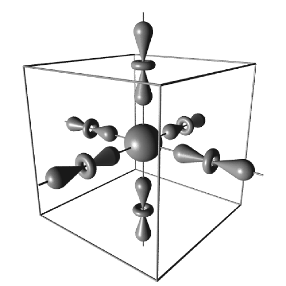
FIG. 5.: Orbital polaron in the strong-coupling limit: Six $e_{g}$ states point towards a central hole.

This configuration also yields a large amplitude of virtual excursions of $e_{g}$ electrons onto the empty site. Thus, besides minimizing the interaction energy of Hamiltonian (28), it also allows to lower the kinetic energy. We note that these virtual hopping processes locally enhance the magnetic moments of core and $e_{g}$ spins via the double-exchange mechanism, providing a large effective spin of the orbital polaron. This naturally explains the development of ferromagnetic clusters experimentally observed at temperatures above $T_{C}$.[18]

B Binding Energy

In conventional lattice-polaron theory, the binding energy is a function of the coupling constant $g$ and the stiffness of the lattice which is controlled by the spring constant $K$: The energy gain stemming from the interaction between charge carriers and the lattice competes against the deformation energy of the crystal. In the case of orbital polarons, the underlying picture is very similar. Here the coupling constant is given by the orbital-charge interaction energy $\Delta$, while the energy scale $W_{\text{orb}}=6xt+J$ is a measure of the “stiffness” of the orbital sector. These two quantities are expected to determine the binding energy of the orbital polaron:

$$E_{b}^{\text{orb}}=f(\Delta,W_{\text{orb}}).$$ (29)

The role of $W_{b}^{\text{orb}}$ can be illustrated as follows (see Fig. 6):

 

FIG. 6.: (a) Orbital fluctuations with an energy scale $\propto xt$ and (b) inter-site correlations $\propto J$ compete against the orbital-hole binding energy $\Delta$.

In an orbital-liquid state, orbitals have to give up part of their fluctuation energy in order to form a bound state with a hole. As a consequence, polarons are stable only if orbital fluctuations are weak. Furthermore, polarons have a frustrating effect on inter-site orbital correlations. The local orientation of orbitals favored by Hamiltonian (28) does in general not comply with the orientation that would minimize the Jahn-Teller and superexchange coupling between orbitals on nearest- and next-nearest-neighbor sites of the hole. Thus, in order to form a bound state orbitals have to give up part of their inter-site correlation energy $J$ as well. The fact that the polaron binding energy is controlled by the orbital energy scale $W_{\text{orb}}=6xt+J$ has direct implications for the phase diagram of manganites: Due to the doping dependence of $W_{\text{orb}}$, orbital polarons are stable only at low hole concentrations where fluctuations are weak. The tendency of the system to form polarons is therefore most pronounced in the lower part of the phase diagram.

To derive an expression for the polaron binding energy, the following approach is used: First we consider a static hole placed in an ordered state without fluctuations. We then calculate the reduction of the total energy due to the interaction Hamiltonian (28). All approximations made in the following aim at discarding terms reminiscent of a specific type of orbital order, while preserving the most general structure of the orbital-hole binding energy. We focus on a single site located next to the hole in the $z$ direction. The orbital configuration at this site is determined by the coupling to the hole described by Eq. (28) as well as by the orientation of neighboring orbitals which couple via superexchange and Jahn-Teller effect; the latter interaction is determined by Hamiltonian (11). Treating all orbitals except the one explicitly considered here on a mean-field level, the following Hamiltonian is obtained for the selected site:

$$H^{z}_{\delta}=-\left(\Delta\tau^{z}_{\delta}+J\tau^{\Theta}_{\delta}\right).$$ (30)

Here $\tau^{\Theta}_{i}=(\sin\Theta\sigma^{x}_{i}+\cos\Theta\sigma^{z}_{i})/2$ fixes the orbital orientation which would minimize the interaction energy with the orbital background — for the type of order used in Eq. (12), e.g., $\Theta=\pm\pi/2$. In general, this orientation does not coincide with the $|3z^{2}-r^{2}\rangle$ configuration favored by the orbital polaron which is described by the first term in brackets. The state actually chosen by the system then depends on the ratio of $\Delta$ and $J$ as well as on the angle $\Theta$. We determine the energy of this state and, since we are not interested in any specific type of order, average over the angle $\Theta$. Finally subtracting the $\Delta\rightarrow 0$ limit and multiplying with the number of bonds connecting the hole to its surrounding, the following expression for the polaron binding energy is obtained:

$$E_{b}^{\text{orb}}=3\left[\sqrt{\Delta^{2}+J^{2}}-J\right].$$ (31)

In the limit $J/\Delta\rightarrow\infty$, the orbital state is very stiff and cannot be polarized by the hole; the binding energy then vanishes as $3\Delta^{2}/(2J)$. On the other hand, the polarization is complete in the limit $J/\Delta\rightarrow 0$, yielding a maximum value $E_{b}^{\text{orb}}=3\Delta$ for the binding energy. A plot of $E_{b}^{\text{orb}}$ is shown in Fig. 7 (upper curve).

FIG. 7.: Polaron binding energy $E_{b}^{\text{orb}}$: The solid curve is a plot of Eq. (31) for the orbitally ordered state as a function of $J$ (upper axis), the dashed curve corresponds to Eq. (38) for the orbital-liquid state and is plotted as a function of $W_{\text{orb}}$ (lower axis).

We note that the functional form of Eq. (31) differs from the conventional lattice-polaron case where $E_{b}^{\text{ph}}=g^{2}/(2K)$. This is due to the fact that there exists an upper limit of the orbital polarization in which the orbitals around a hole have been fully reoriented to point towards the empty site (see Fig. 5); technically the existence of this upper bound is reflected by the hard-core nature of the Pauli operators in Eq. (30). The familiar form of the binding energy $\propto\Delta^{2}/J$ is recovered only for the weak-coupling limit in which orbital distortions around the hole are small.

Next we consider a static hole placed in a strongly fluctuating orbital-liquid state. Hamiltonian (28) imposes a splitting of $e_{g}$ levels on the sites next to the hole. The orbiton quasiparticles of Sec. II scatter on these local potentials, which may lead to the formation of an orbiton-hole bound state. To calculate the polaron stabilization energy we again consider a single site next to the hole in the $z$ direction. The local potential imposed by the close-by hole is of the form

$$H^{z}_{\delta}=-\Delta\tau^{z}_{\delta},$$ (32)

where $\tau^{z}_{i}=\frac{1}{2}\sigma^{z}_{i}$. We calculate the effect of successive scattering of orbitons on the above potential employing a $T$-matrix formalism; interference between different scattering centers is neglected here. The correction to the orbiton Green’s function that seizes the effect of Hamiltonian (32) is given by

$$\delta G_{\text{orb}}(i\omega;\mathchoice{{\hbox{\boldmath$\displaystyle R$}}}{{\hbox{\boldmath$\textstyle R$}}}{{\hbox{\boldmath$\scriptstyle R$}}}{{\hbox{\boldmath$\scriptscriptstyle R$}}},\mathchoice{{\hbox{\boldmath$\displaystyle R$}}}{{\hbox{\boldmath$\textstyle R$}}}{{\hbox{\boldmath$\scriptstyle R$}}}{{\hbox{\boldmath$\scriptscriptstyle R$}}})=G^{0}_{\text{orb}}(i\omega;\mathchoice{{\hbox{\boldmath$\displaystyle R$}}}{{\hbox{\boldmath$\textstyle R$}}}{{\hbox{\boldmath$\scriptstyle R$}}}{{\hbox{\boldmath$\scriptscriptstyle R$}}},\delta)T_{\delta}(i\omega)G^{0}_{\text{orb}}(i\omega;\delta,\mathchoice{{\hbox{\boldmath$\displaystyle R$}}}{{\hbox{\boldmath$\textstyle R$}}}{{\hbox{\boldmath$\scriptstyle R$}}}{{\hbox{\boldmath$\scriptscriptstyle R$}}}),$$ (33)

with the scattering matrix

$\displaystyle T_{\delta}(i\omega)=-\frac{\sigma^{z}\Delta/2}{1-\sigma^{z}\Delta G^{0}_{\text{orb}}(i\omega)/2}.$

Here $G^{0}_{\text{orb}}(i\omega;\mathchoice{{\hbox{\boldmath$\displaystyle R$}}}{{\hbox{\boldmath$\textstyle R$}}}{{\hbox{\boldmath$\scriptstyle R$}}}{{\hbox{\boldmath$\scriptscriptstyle R$}}},\mathchoice{{\hbox{\boldmath$\displaystyle R$}}}{{\hbox{\boldmath$\textstyle R$}}}{{\hbox{\boldmath$\scriptstyle R$}}}{{\hbox{\boldmath$\scriptscriptstyle R$}}}^{\prime})$ denotes the orbiton propagator of the system in the absence of the scattering potential. The elements of this 2$\times$2 matrix are given by $[G^{0}_{\text{orb}}(i\omega;\mathchoice{{\hbox{\boldmath$\displaystyle R$}}}{{\hbox{\boldmath$\textstyle R$}}}{{\hbox{\boldmath$\scriptstyle R$}}}{{\hbox{\boldmath$\scriptscriptstyle R$}}},\mathchoice{{\hbox{\boldmath$\displaystyle R$}}}{{\hbox{\boldmath$\textstyle R$}}}{{\hbox{\boldmath$\scriptstyle R$}}}{{\hbox{\boldmath$\scriptscriptstyle R$}}}^{\prime})]^{\alpha\beta}=-\langle T_{\tau}f_{\mathchoice{{\hbox{\boldmath$\displaystyle R$}}}{{\hbox{\boldmath$\textstyle R$}}}{{\hbox{\boldmath$\scriptstyle R$}}}{{\hbox{\boldmath$\scriptscriptstyle R$}}}\alpha}f^{\dagger}_{\mathchoice{{\hbox{\boldmath$\displaystyle R$}}}{{\hbox{\boldmath$\textstyle R$}}}{{\hbox{\boldmath$\scriptstyle R$}}}{{\hbox{\boldmath$\scriptscriptstyle R$}}}^{\prime}\beta}\rangle^{0}_{i\omega}$ and are controlled by the mean-field Hamiltonian (5). The on-site Green’s function is $G^{0}_{\text{orb}}(i\omega)=\frac{1}{2}\text{Tr}[G^{0}_{\text{orb}}(i\omega;\delta,\delta)]$. Integrating over lattice sites, Eq. (33) becomes

$$\delta G(i\omega) = -\frac{\Delta}{4}\left[\frac{\partial}{\partial i\omega}G^{0}(i\omega)\right]$$ (35)

$$\times\left(\frac{1}{1-\Delta G^{0}(i\omega)/2}-\frac{1}{1+\Delta G^{0}(i\omega)/2}\right),$$

with $\delta G_{\text{orb}}(i\omega)=\frac{1}{2}\sum_{\mathchoice{{\hbox{\boldmath$\displaystyle R$}}}{{\hbox{\boldmath$\textstyle R$}}}{{\hbox{\boldmath$\scriptstyle R$}}}{{\hbox{\boldmath$\scriptscriptstyle R$}}}}\text{Tr}[\delta G_{\text{orb}}(i\omega;\mathchoice{{\hbox{\boldmath$\displaystyle R$}}}{{\hbox{\boldmath$\textstyle R$}}}{{\hbox{\boldmath$\scriptstyle R$}}}{{\hbox{\boldmath$\scriptscriptstyle R$}}},\mathchoice{{\hbox{\boldmath$\displaystyle R$}}}{{\hbox{\boldmath$\textstyle R$}}}{{\hbox{\boldmath$\scriptstyle R$}}}{{\hbox{\boldmath$\scriptscriptstyle R$}}})]$. The change in the total energy of the system which is induced by the scattering potential can now be obtained from Eq. (35) by employing

$$\delta E=2\int_{-\infty}^{\mu}dw\;(\omega-\mu)\;\delta\rho(\omega),$$ (36)

where $\delta\rho(\omega)=-(1/\pi)\text{Im}[\delta G(i\omega\rightarrow\omega+i0^{+})]$ denotes the scattering contribution to the density of states. The orbiton chemical potential is set to $\mu=0$ in the following. We evaluate Eq. (36) by approximating the on-site Green’s function by

$$G^{0}(i\omega)\approx-\frac{1}{W_{\text{orb}}}\ln\left[\frac{i\omega-W_{\text{orb}}/2}{i\omega+W_{\text{orb}}/2}\right].$$ (37)

This expression yields a constant density of states for the translationally invariant system which resembles the result that can be obtained numerically from the mean-field Hamiltonian (5). Approximately solving the integral in Eq. (36) and multiplying the result with the number of nearest neighbors of the hole, we finally arrive at the following expression for the polaron binding energy:

$$E_{b}^{\text{orb}}=3\Delta\left[y\left(\text{cth}\,y-1\right)+\frac{y\ln 2}{y^{2}+(\pi/2)^{2}}\right],$$ (38)

with $y=W_{\text{orb}}/\Delta$. Equation (38) describes the polaron stabilization energy in a strongly fluctuating orbital-liquid state. A plot of this function is shown in Fig. 7 (lower curve). The binding energy reaches its maximum $E_{b}^{\text{orb}}=3\Delta$ if orbital fluctuations are weak, while it vanishes as $3\ln 2(\Delta^{2}/W_{\text{orb}})$ in the opposite limit where fluctuations are strong.

In the last two paragraphs we have calculated the polaron binding energy in an orbitally ordered as well as in an orbital-liquid state. Although very different approaches were used to describe these complementary cases, the expressions obtained closely coincide: As can be seen in Fig. 7, the two functions are almost indistinguishable if one identifies $J$ in Eq. (31) with $\nu W_{\text{orb}}$ in Eq. (38), where $\nu\approx 0.72$ is a numerical fitting factor. Motivated by the observation that $W_{\text{orb}}=6xt+J$ reduces to $J$ in the limit of strong orbital correlations $J\gg xt$, we discard the fitting factor in the following by setting $\nu=1$. We believe these two cases to be smoothly connected as should come out in a more elaborate treatment of the problem. Based upon these considerations, we conclude that Eq. (31) can be used to model the polaron binding energy of both the fluctuating and the static orbital state:

$$E_{b}^{\text{orb}}=3(1-x)\left[\sqrt{\Delta^{2}+W_{\text{orb}}^{2}}-W_{\text{orb}}\right],$$ (39)

where $W_{\text{orb}}=6xt+J$ in former and $W_{\text{orb}}=J$ in the latter case. We finally note that in deriving expressions (31) and (38) for the binding energy, all six sites surrounding the static hole were assumed to be occupied. Since at finite doping the probability of a site being occupied is only $(1-x)$, we renormalize Eq. (39) by this average occupation factor.

To summarize, $E_{b}^{\text{orb}}$ in Eq. (39) represents the energy to be gained by polarizing the orbital background around a static hole. This number depends on the orbital energy scale $W_{\text{orb}}=6xt+J$, i.e., on orbital fluctuations and inter-site orbital correlations which both tend to suppress the polaron binding energy. $W_{\text{orb}}$ is to be considered as the counterpart of the lattice stiffness $K$ in conventional polaron theory. The important difference is that $W_{\text{orb}}$ explicitly depends on $x$ which has important consequences for the phase diagram of manganites: Orbital polarons can form only at low doping concentrations where orbital fluctuations are weak and the binding energy is consequently large.

C Polaron Bandwidth

The orbitally degenerate Mott-Hubbard system is instable towards the formation of orbital-hole bound states at low doping concentrations. In this small-polaron regime, holes are pinned by the binding potential and can move only if being thermally activated. At low temperatures these processes can be neglected; coherent charge motion is then possible solely due to quantum tunneling. Since the polaron is a composite object consisting of a hole and several orbitals, the amplitude of these tunneling processes is expected to be small as is indeed shown in this section.

Here we restrict ourselves to polarons moving in an orbitally ordered state. Our analysis is based upon the following idea: By allowing a hole to polarize the surrounding orbitals, the system reduces its ground state energy by $E_{b}^{\text{orb}}$. This energy is mostly lost if the hole hops to another site since the orbital sector cannot immediately adopt to the new position — orbital fluctuations are slow compared to those of holes. After a short time the system returns to the ground state, most likely by transferring the hole back to its original location. But there is also a small probability for the hole to keep its new position while the orbital sector adapts to the relocation. This is possible due to the non-orthogonality of configurations in which orbitals point towards the old and the new location of the hole, respectively. The polaron tunneling amplitude is then given by the transfer amplitude $t$ of holes multiplied by the overlap between states with orbitals pointing towards the old and new position of the hole, respectively. This overlap is calculated as follows: We use Hamiltonian (30) to determine the orientation of a single orbital next to the hole — all other orbitals are treated on a mean-field level. As the hole hops, this orbital has to change its orientation from pointing towards the hole to being aligned with the background. The projection between these two states is

$$p=\frac{1}{\sqrt{2}}\left[1+\frac{J}{\sqrt{\Delta^{2}+J^{2}}}\right]^{1/2}.$$ (40)

An average over the angle $\Theta$ specifying the type of orbital order in Eq. (30) has been performed here. Other orbitals undergo the reversed process: Originally being aligned with the background, they turn towards the hole as the latter hops onto a neighboring site. In total there are $2(z-1)\approx 2z$ orbitals that have to reorient. The overlap between the initial and the final state is then given by $P=p^{2z}$, yielding

$$P=\frac{1}{2^{z}}\left[1+\frac{J}{\sqrt{\Delta^{2}+J^{2}}}\right]^{z}.$$ (41)

We rewrite Eq. (41) as

$$P = \left[1-\frac{\sqrt{\Delta^{2}+J^{2}}-J}{2\sqrt{\Delta^{2}+J^{2}}}\right]^{z}$$ (42)

$$\approx \exp\left[-3\frac{\sqrt{\Delta^{2}+J^{2}}-J}{\sqrt{\Delta^{2}+J^{2}}}\right],$$ (43)

where the exponential form becomes exact for large coordination number which has been set to $z=6$. The denominator in the exponent is identified as the orbital binding energy given by Eq. (31). Hence we finally arrive at the following compact expression for $P\equiv e^{-\eta}$:

$$e^{-\eta}=\exp\left[-\frac{E_{b}^{\text{orb}}}{\sqrt{\Delta^{2}+J^{2}}}\right].$$ (44)

A plot of this function is shown in Fig. 8.

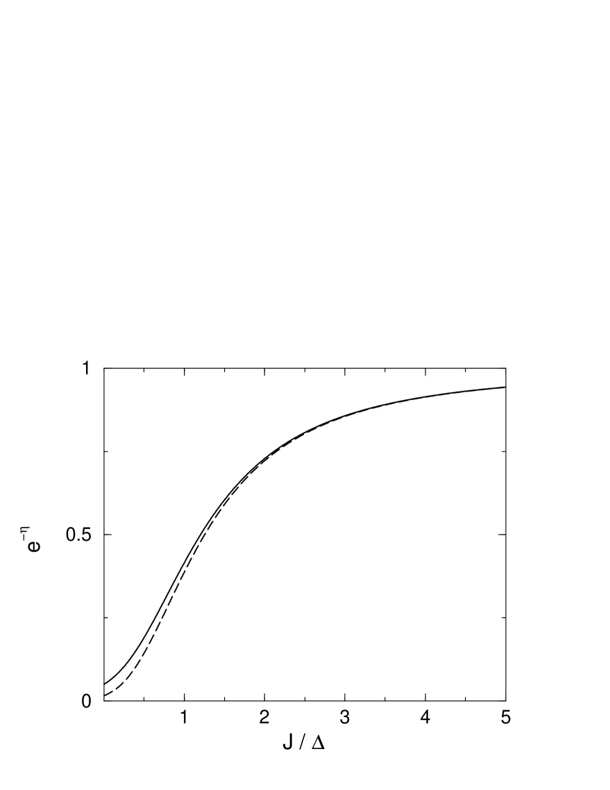
FIG. 8.: Ratio of polaron and holon bandwidth $e^{-\eta}$. The solid line is based on the exponential form in Eq. (44), the dashed line represents Eq. (41). The polaron bandwidth shrinks which decreasing values of $J/\Delta$ associated with an enhanced orbital polarizability.

The physical significance of $e^{-\eta}$ is that it relates the holon to the polaron bandwidth:

$$W_{\text{pol}}=W_{\text{hl}}\;e^{-\eta}.$$ (45)

As the system becomes critical towards the formation of orbital-hole bound states, polarons replace holes as charge carriers. Our result shows that this transition is accompanied by an exponential suppression of the bandwidth. Strictly speaking the translationally invariant system remains a metal; in reality, however, the small bandwidth makes polarons susceptible to localization, e.g., by trapping in the random potential of impurities. The suppression of the bandwidth is most pronounced if the polaron binding energy is large: The orbitals around the hole are then strongly distorted, which necessitates a significant reorientation to allow the hole to hop. We note that the expression in Eq. (44) is similar to the result obtained in conventional lattice-polaron theory where $e^{-\eta}=\exp\left(-E_{b}^{\text{ph}}/\omega_{0}\right)$. Here $E_{b}^{\text{ph}}=g^{2}/(2K)$ denotes the polaron binding energy and $\omega_{0}$ the phonon frequency; the latter corresponds to $(\Delta^{2}+J^{2})^{1/2}$ in our orbital-polaron theory.

Equation (44) has been derived for a static, non-fluctuating orbital state. Following the discussion in deriving the polaron binding energy, we generalize the result to account for orbital fluctuations as well. This is done by replacing the inter-site correlation energy $J$ by the more general orbital energy scale $W_{\text{orb}}=6xt+J$. Hence we obtain

$$e^{-\eta}=\exp\left[-\frac{E_{b}^{\text{orb}}}{\sqrt{\Delta^{2}+W_{\text{orb}}^{2}}}\right],$$ (46)

where the polaron binding energy $E_{b}^{\text{orb}}$ is now given by Eq. (39).

To summarize, the development of orbital polarons leads to a sharp reduction of the bandwidth. In this regime the orbital-hole bound state can move only as an entity via quantum-tunneling processes. Since the polaron extends over several lattice sites, the transfer amplitude is exponentially small. The bandwidth reduction is controlled by the ratio $E_{b}^{\text{orb}}/[\Delta^{2}+W_{\text{orb}}^{2}]^{1/2}$ which is a measure of the orbital distortions around a hole. Strong orbital fluctuations and inter-site orbital correlations weaken the polaron effect by suppressing these distortions.

IV Metal-Insulator Transition

As was shown in the preceeding section, the formation of orbital-hole bound states leads to an exponential suppression of the bandwidth which makes the system prone to localization. In a double-exchange system, this crossover from a free-carrier to a small-polaron picture can be initiated either by a reduction of the doping concentration or by an increase in temperature; the former acts via an enhancement of the polaron binding energy, the latter by constricting the motion of holes via the double-exchange mechanism. In this section we combine our orbital-polaron picture with the theory of conventional lattice polarons to develop a scheme of the metal-insulator transition in manganites.

The transition from a free-carrier to a small-polaron picture is governed by the dimensionless coupling constant $\lambda_{\text{orb}}=E_{b}^{\text{orb}}/D_{\text{hl}}$, where $E_{b}^{\text{orb}}$ is the polaron binding energy given by Eq. (39) and $D_{\text{hl}}=W_{\text{hl}}/2=3t$ is the half-bandwidth of holes. The lattice breathing mode of Eq. (25) adds an additional contribution $\lambda_{\text{ph}}=E_{b}^{\text{ph}}/D_{\text{hl}}$ with $E_{b}^{\text{ph}}=g_{1}^{2}/(2K)$, which further promotes the formation of polarons. The coupling constant thus becomes

$$\lambda=\frac{E_{b}^{\text{orb}}+E_{b}^{\text{ph}}}{D_{\text{hl}}}.$$ (47)

The critical value that separates free-carrier and small-polaron regimes is $\lambda=1$. For $\lambda\gg 1$ small polarons have fully developed and the bandwidth is reduced by an exponential factor

$$e^{-\eta}=\exp\left[-\gamma\left(\frac{E_{b}^{\text{orb}}}{\sqrt{\Delta^{2}+W_{\text{orb}}^{2}}}+\frac{E_{b}^{\text{ph}}}{\omega_{0}}\right)\right],$$ (48)

with $\gamma=1$. We note that interference effects between orbital and lattice coupling are neglected in Eq. (48). For $\lambda<1$ the free-carrier picture is recovered and holes move in a band of width $W_{\text{hl}}=6t$. This implies $\gamma=0$ in Eq. (48), yielding $e^{-\eta}=1$. To simulate the crossover between the two regimes, we phenomenologically employ the function

$$\gamma=\left\{\begin{array}[]{l}\displaystyle\beta-\frac{\ln[\lambda(1+\beta)]}{\lambda^{2}}\quad\text{for}\quad\lambda>1,\\[12.0pt] \displaystyle 0\quad\text{for}\quad\lambda<1,\end{array}\right.$$ (49)

with $\beta=[1-1/\lambda^{2}]^{1/2}$. This function has been proposed for strongly coupled electron-phonon systems (see, e.g., Ref. [19]) and avoids an unphysical sudden drop of the bandwidth as $\lambda=1$ is reached. The crossover hence obtained for $e^{-\eta}$ is depicted in Fig. 9.

FIG. 9.: Crossover from the free-carrier to the small-polarons regime. At $\lambda<1$ polarons are unstable and the bare holon bandwidth is recovered. At $\lambda>1$ orbital polarons form, leading to an exponential suppression of the bandwidth. To avoid an abrupt drop of the bandwidth at $\lambda=1$, Eq. (49) is used to connect the two regimes.

Up to this point we have mainly focused on the role of the orbital energy scale $W_{\text{orb}}$ in the formation of small polarons. We now turn to analyze in more detail the effect of temperature. The latter controls the bandwidth $W_{\text{hl}}$ via the double-exchange mechanism: At low temperatures all spins are ferromagnetically aligned and the transfer amplitude reaches its maximum. With increasing temperature the ferromagnetic moment weakens, constricting the motion of charge carriers. Specifically, the transfer amplitude changes with the normalized magnetization $m$ as

$$t=t_{0}\sqrt{(1+m^{2})/2}.$$ (50)

The magnetization depends on temperature via the self-consistent equation

$$m=B_{S}(\alpha m)\quad\text{with}\quad\alpha=\frac{3S}{1+S}\;\frac{T_{C}}{T},$$ (51)

where

$\displaystyle B_{S}(y)=\frac{2S+1}{2S}\;\text{cth}\left[\frac{2S+1}{2S}\;y\right]-\frac{1}{2S}\;\text{cth}\left[\frac{1}{2S}\;y\right]$

denotes the Brillouin function. The average magnetic moment per site varies with doping: The moments $S^{c}=3/2$ and $s=1/2$ of core and $e_{g}$ spins combine on average as

$$S=\frac{3}{2}+\frac{1}{2}(1-x).$$ (52)

Finally, the Curie temperature $T_{C}$ in Eq. (51) is controlled by the strength $J_{\text{eff}}$ of ferromagnetic exchange bonds via

$$T_{C}=\frac{\nu z}{3}S(S+1)J_{\text{eff}}.$$ (53)

The fitting parameter $\nu$ compensates for an overestimation of $T_{C}$ in the mean-field treatment. Double-exchange as well as superexchange processes are responsible for establishing the ferromagnetic links between sites. The magnitude of this coupling in the limit of large Hund’s coupling is[11]

$$J_{\text{eff}}=\frac{1}{2S^{2}}\left[x(1-x)\chi te^{-\eta}+(1-x)^{2}\frac{2\chi^{2}t_{0}^{2}}{U}\right].$$ (54)

The first term in squared brackets of Eq. (54) stems from the coherent motion of holes/polarons and represents the conventional double-exchange contribution to $T_{C}$. The factor $e^{-\eta}$ accounts for the rescaling of the coherent bandwidth as the small-polaron regime is entered. The second term is due to superexchange processes. It describes the high-energy virtual hopping of $e_{g}$ electrons which is insensitive to a polaronic reduction of the bandwidth. It is also noticed that superexchange in an orbitally degenerate system is of ferromagnetic nature because of the large Hund’s coupling present in manganites.[11, 20, 21] Superexchange hence dominates the ferromagnetic interaction in the small-polaron regime.

The system of equations presented above controls the electronic and magnetic behavior of manganites at low and intermediate doping levels. A critical coupling $\lambda=1$ leading to the formation of polarons can be reached either by lowering the doping concentration or by increasing the temperature — the former enhances $E_{b}^{\text{orb}}$, the latter quenches $W_{\text{hl}}$. The equations are interrelated and have to be solved recursively. As a result of this self consistency, the breakdown of the metallic bandwidth at $\lambda=1$ is expected to be rather sharp: With the evolution of small polarons, the coherent band width shrinks, thereby weakening the magnetic exchange links. Double exchange then drives the system even farther towards the strong-coupling limit.

V Comparison with Experiment

To illustrate the interplay between the system of equations presented in the preceeding section, we numerically extract from them the $T$-$x$ phase diagram. While it is obvious that $T=T_{C}$ is a suitable criterion to separate the low-temperature ferromagnetic from the high-temperature paramagnetic state, more care has to be taken to distinguish between metallic and insulating behavior. Our theory describes the reduction of the bandwidth which follows from the formation of small polarons. However, strictly speaking, the system remains metallic even in the strong-coupling limit since polarons can still move by tunneling. It is therefore necessary to define a critical value of the bandwidth beyond which additional effects such as pinning to impurities are implicitly assumed to set in and finally turn the system into an insulator. The specific criterion used here is only of marginal importance, as feedback effects discussed above induce a quick collapse of the bandwidth once a critical coupling $\lambda=1$ is reached. For simplicity we define $\lambda<1$ to be a metal and $\lambda>1$ to be an insulator.

The following parameters are chosen for calculating the phase diagram: The orbital polarization energy is set to $\Delta=0.55~{}\text{eV}$, yielding a binding energy comparable to the phononic one $E_{b}^{\text{ph}}=0.45~{}\text{eV}$; the phonon frequency is $\omega_{0}=0.05~{}\text{eV}$, the interaction between orbitals $J=0.13~{}\text{eV}$, the bare transfer amplitude $t_{0}=0.36~{}\text{eV}$,[8] and $U=4.0$ eV. The fitting parameter $\nu=0.55$ (Ref. [22]) is adjusted to reproduce the values of $T_{C}$ observed for La_1-xSr_xMnO₃.[23] The result is shown in Fig. 10.

FIG. 10.: Magnetic and electronic phase diagram obtained within the present theory. Dashed and dot-dashed lines represent magnetic and electronic transitions, respectively, the simultaneous transition in both channels is denoted by a solid line. The phases are: paramagnetic insulator (PI), paramagnetic metal (PM), ferromagnetic metal (FM), and ferromagnetic insulator (FI).

Our most important observation is that the doping dependence of orbital polarons makes the system more insulating at low and more metallic at high doping levels. Convincingly this is seen in the complete absence of metalicity at $x<0.15$ and the appearance of a metallic phase above $T_{C}$ at $x>0.4$. The region $0.15<x<0.4$ in which colossal magnetoresistance is experimentally observed is characterized by a simultaneous magnetic and electronic transition from a ferromagnetic metal to a paramagnetic insulator.[24] The role of polarons in this transition is most pronounced at low hole concentrations. This can be seen from the behavior of the magnetization as $T_{C}$ is approached from below (see Fig. 11):

FIG. 11.: Variation of the normalized magnetization $m$ with temperature. At low hole concentrations (upper curve), the system is close to a transition to the small-polaron regime — a small increase in temperature then already sufficiently impedes the hole motion for polarons to form, resulting in a sharp drop of the magnetization. At large $x$ (lower curve), the conventional double-exchange picture is recovered.

At low $x$, the polaron binding energy is large and the system is close to localization. A small reduction of the bandwidth via double exchange is then sufficient to trigger the formation of polarons, resulting in a sudden collapse of the magnetic moment. Such a sharp drop signals the presence of a localization mechanism beyond double exchange and is indeed seen experimentally (see, e.g., Refs. [24, 25, 26]). On the other hand, at larger hole concentrations the polaron binding energy is comparably small. Thus, a significant suppression of the bandwidth via double exchange is needed before polaron formation can set in. The magnetization curve now closely resembles the one predicted by double-exchange theory.

Clearly beyond the grasp of conventional double-exchange theory lies the emergence of ferromagnetism in the insulating phase at low doping. Mostly responsible for this are superexchange processes which mediate a ferromagnetic interaction even in the insulating phase. Ferromagnetism is further promoted by the existence of orbital polarons: Charge fluctuations inside the polaron provide a strong local ferromagnetic coupling between sites close to a hole, hence establishing ferromagnetic clusters seen in experiment.[18] At sufficiently large hole densities these clusters start to interact, thereby forming a ferromagnetic state.

As was discussed above, orbital fluctuations are predominantly induced by the motion of holes. The loss of charge mobility in the insulating phase should therefore trigger static orbital order. An orbitally ordered state has in fact been experimentally detected in the insulating regions of La_0.88Sr_0.12MnO₃.[20] However, in general such an ordered state is expected to have orbital and Jahn-Teller glass features due to the presence of quenched orbital polarons, thereby reducing the uniform component of Jahn-Teller distortions. Finally it is worth to notice that the phase diagram in this theory is highly sensitive to the transfer amplitude $t_{0}$ as this parameter enters in the polaron binding energy.

VI Conclusion

In summary, we have shown that a spontaneous development of orbital-lattice order is in general insufficient to trigger the localization process in manganites. Rather an additional mechanism was identified: Orbital polarons were illustrated to represent an intrinsic feature of an orbitally degenerate Mott-Hubbard system and to play an important role in the physics of manganites. The binding energy of these orbital-hole bound states depends on the rate of orbital fluctuations and hence on the concentration of doped holes: Polarons can form at low doping levels where orbitals fluctuate only weakly but they become unstable at higher levels of $x$. This scheme naturally introduces the hole concentration as an additional variable into the localization process. Most striking in this respect is the complete breakdown of metalicity observed below a critical hole concentration despite the fact that the system remains ferromagnetically ordered. On the other hand, orbital polarons become negligible at larger doping levels where the theory presented here converges onto a lattice-polaron double-exchange picture. Accounting for both orbital and lattice effects we are finally able to reproduce well the important aspects of the phase diagram of manganites. In general it can be concluded that a direct coupling between holes and surrounding orbitals is of crucial importance for the physics of manganites; its implications extend clearly beyond the metallic phase alone and can be expected to play an important role throughout the whole phase diagram.

REFERENCES

- [1] C. Zener, Phys. Rev. 82, 403 (1951); P. W. Anderson and H. Hasegawa, ibid. 100, 675 (1955); P.-G. de Gennes, ibid. 118, 141 (1960).
- [2] A. J. Millis, B. I. Shraiman, and R. Mueller, Phys. Rev. Lett. 77, 175 (1996); A. J. Millis, Nature (London) 392, 147 (1998).
- [3] J. H. Röder, J. Zang, and A. R. Bishop, Phys. Rev. Lett. 76, 1356 (1996).
- [4] C. M. Varma, Phys. Rev. B 54, 7328 (1996).
- [5] M. Capone, M. Grilli, and W. Stephan, J. Superconductivity 12, 75 (1999); cond-mat/9902317 (unpublished).
- [6] E. Dagotto, Rev. Mod. Phys. 66, 763 (1994).
- [7] S. Ishihara, J. Inoue, and S. Maekawa, Phys. Rev. B 55, 8280 (1997).
- [8] R. Kilian and G. Khaliullin, Phys. Rev. B 58, R11 841 (1998).
- [9] K. Kubo and A. Ohata, J. Phys. Soc. Jpn. 33, 21 (1972).
- [10] S. Ishihara, M. Yamanaka, and N. Nagaosa, Phys. Rev. B 56, 686 (1997).
- [11] G. Khaliullin and R. Kilian, cond-mat/9904316 (unpublished).
- [12] Y. Murakami, J. P. Gill, D. Gibbs, M. Blume, I. Koyama, M. Tanaka, H. Kawata, T. Arima, Y. Tokura, K. Hirota, and Y. Endoh, Phys. Rev. Lett. 81, 582 (1998).
- [13] C. L. Kane, P. A. Lee, and N. Read, Phys. Rev. B 39, 6880 (1989).
- [14] G. Martinez and P. Horsch, Phys. Rev. B 91, 317 (1991).
- [15] The factor in Eq. (22) compensates only partially for the mean-field treatment of the constraint that forbids more than one orbital excitation per site. The bandwidth numerically obtained for is therefore slightly larger than .
- [16] D. S. Dessau and Z.-X. Shen, in Colossal Magnetoresistive Oxides, edited by Y. Tokura (Gordon and Breach, Newark, 1998).
- [17] S. Saitoh, A. E. Bocquet, T. Mizokawa, H. Namatame, A. Fujimori, M. Abbate, Y. Takeda, and M. Takano, Phys. Rev. B 51, 13 942 (1995).
- [18] J. M. De Teresa, M. R. Ibarra, P. A. Algarabel, C. Ritter, C. Marquina, J. Blasco, J. Garcia, A. del Moral, and Z. Arnold, Nature (London) 386, 256 (1997).
- [19] A. S. Alexandrov, V. V. Kabanov, and D. K. Ray, Phys. Rev. B 49, 9915 (1994).
- [20] Y. Endoh, K. Hirota, S. Ishihara, S. Okamoto, Y. Murakami, A. Nishizawa, T. Fukuda, H. Kimura, H. Nojiri, K. Kaneko, and S. Maekawa, Phys. Rev. Lett. 82, 4328 (1999).
- [21] R. Maezono, S. Ishihara, and N. Nagaosa, Phys. Rev. B 58, 11 583 (1998).
- [22] This factor is partly attributed to the fluctuation correction to the mean-field value of which follows from Eq. (5.4) in G. S. Rushbrooke, G. A. Baker, and P. J. Wood, in Phase Transitions and Critical Phenomena, edited by C. Domb and M. S. Green (Academic, New York, 1974).
- [23] A. Urushibara, Y. Moritomo, T. Arima, A. Asamitsu, G. Kido, and Y. Tokura, Phys. Rev. B 51, 14 103 (1995).
- [24] P. Schiffer, A. P. Ramirez, W. Bao, and S.-W. Cheong, Phys. Rev. Lett. 75, 3336 (1995).
- [25] G. M. Zhao, K. Conder, H. Keller, and K. A. Müller, Nature (London) 381, 676 (1996).
- [26] J. P. Franck, I. Isaac, W. Chen, J. Chrzanowski, J. C. Irwin, and C. C. Homes, J. Superconductivity 12, 263 (1999).