Low-density series expansions for directed percolation I:
A new efficient algorithm with applications to the square lattice

Abstract

A new algorithm for the derivation of low-density series for percolation on directed lattices is introduced and applied to the square lattice bond and site problems. Numerical evidence shows that the computational complexity grows exponentially, but with a growth factor $\lambda<{\sqrt[8]{2}}$, which is much smaller than the growth factor $\lambda={\sqrt[4]{2}}$ of the previous best algorithm. For bond (site) percolation on the directed square lattice the series has been extended to order 171 (158). Analysis of the series yields sharper estimates of the critical points and exponents.

1 Introduction

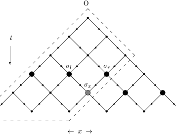
Figure 1: The directed square lattice with orientation given by the arrows.

Directed percolation (DP) [1, 2] can be thought of as a purely geometric model in which the bonds or sites of a hyper-cubic lattice ${\mathbb{Z}}^{d}$ are either present with probability $p$ or absent (with probability $q=1-p$). Unless otherwise specified I shall be looking at bond percolation on the directed square lattice. As in ordinary percolation one might be interested in the average cluster-size $S(p)$. The difference is that in DP connections are only allowed along a preferred direction given by an orientation of the edges. Fig. 1 shows the part of the square lattice which can be reached from the origin using no more than five steps. Apart from the inherent theoretical interest DP has been associated with a wide variety of physical phenomena. In static interpretations, the preferred direction is spatial, and DP could model gravity driven percolation of fluid through porous rock with a certain fraction of the channels blocked [3], crack propagation [4] or electric current in a diluted diode network [5]. In dynamical interpretations, the preferred direction is time and one realization is as a model of an epidemic without immunization. DP type transitions are also encountered in many other situations including Reggeon field theory [6], chemical reactions [7], heterogeneous catalysis and other surface reactions [8], self-organized criticality [9], and even galactic evolution [10].

Domany and Kinzel [11] demonstrated that bond percolation on the directed square lattice is a special case of a one-dimensional stochastic cellular automaton. The evolution of the model is governed by the transition probabilities $W(\sigma_{x}|\sigma_{l},\sigma_{r})$, with $\sigma_{i}=1$ if site $i$ is occupied and 0 otherwise. It is the probability of the site $x$ being in state $\sigma_{x}$ at time $t$ given that the sites $x-1$ and $x+1$ at time $t-1$ were in states $\sigma_{l}$ and $\sigma_{r}$, respectively. One has a free hand in choosing the transition probabilities as long as one respects conservation of probability, $P(1|\sigma_{l},\sigma_{r})=1-P(0|\sigma_{l},\sigma_{r})$. Bond percolation corresponds to the choice:

$$W(0|\sigma_{l},\sigma_{r})=(1-p)^{\sigma_{l}+\sigma_{r}}$$ (1)

Note that while one talks of occupied sites in the cellular automata language, the choice of $W$ above does indeed correspond to bond percolation in the static version, as can easily be verified by explicitly looking at all possible configurations and their associated probabilities.

The behavior of the model is controlled by the branching probability (or density of bonds) $p$. When $p$ is smaller than a critical value $p_{c}$ all clusters remain finite. Above $p_{c}$ there is a non-zero probability of finding an infinite cluster and $S(p)$ diverges as $p\rightarrow p_{c}^{-}$. In the low-density phase ($p<p_{c}$) many quantities of interest can be derived from the pair-connectedness $C_{x,t}(p)$, which is the probability that the site $x$ is occupied at time $t$ given that the origin was occupied at $t=0$. The moments of the pair-connectedness may be written as

$$\mu_{n,m}(p)=\sum_{t=0}^{\infty}\sum_{x}x^{n}t^{m}C_{x,t}(p).$$ (2)

In particular the average cluster size $S(p)=\mu_{0,0}(p)$. Due to symmetry, moments involving odd powers of $x$ vanish. The remaining moments diverge as $p$ approaches the critical point from below:

$$\mu_{n,m}(p)\propto(p_{c}-p)^{-(\gamma+n\nu_{\perp}+m\nu_{\parallel})},\;\;\;\;p\rightarrow p_{c}^{-}.$$ (3)

For isotropic percolation many exact results are known for two-dimensional systems, e.g., the critical exponents are known exactly from arguments based on conformal field theory [13] and for some lattices the critical point is known exactly [12]. Isotropic bond percolation is also related to the $q\rightarrow 1$ limit of the Potts model [14, 15]. For directed percolation no such exact results are known, except for special limited versions such as compact directed percolation [16]. Though it is worth mentioning that directed bond percolation is related to the $q\rightarrow 1$ limit of the chiral Potts model [17] and to the $m\rightarrow 0$ limit of the $m$-friendly walker problem [18, 19]. So in order to study directed percolation one has to resort to numerical methods. For many problems the method of series expansions is by far the most powerful method of approximation. For other problems Monte Carlo methods are superior. For the study of DP on two-dimensional lattices, series analysis is undoubtedly the most appropriate choice. This method consists of calculating the first coefficients in the expansion of $\mu_{n,m}(p)$. Given such a series, using the numerical technique known as differential approximants [20], highly accurate estimates can frequently be obtained for the critical point and exponents, as well as the location and critical exponents of possible non-physical singularities.

The difficulty in the enumeration of most interesting lattice problems is that, computationally, they are of exponential complexity. Initial efforts at computer enumeration of square lattice directed percolation were based on direct counting. The computational complexity is proportional to $\lambda_{1}^{n},$ where $n$ is the number of terms in the series, and $\lambda_{1}=3$, is the connective constant for directed lattice animals on the square lattice [21]. A dramatic improvement was achieved by the transfer matrix technique of Blease who devised an algorithm with a complexity, which is proportional to $\lambda_{2}^{n},$ where $\lambda_{2}=\sqrt{2}\approx 1.414.$ This work resulted in a derivation of the first 21 terms in the low-density series on the square lattice. Over the years further significant progress was obtained by Essam and co-workers who supplemented the transfer matrix technique by a weak subgraph expansion and obtained first 25 terms [23] and some years later 35 terms [24]. Note that while the weak subgraph expansion enables one to derive more terms it does not improve the computational complexity. Eventually they devised a resummation technique [25] which was used to derive the so-called non-nodal graph expansion [26]. This in turn enabled them to obtain twice as many terms [25] as could be obtained by the bare algorithm of Blease, resulting in a series of 49 terms. So this approach has a complexity, which is proportional to $\lambda_{3}^{n},$ where $\lambda_{3}=\sqrt[4]{2}\approx 1.189.$ This method was later supplemented by an extension method [27], originally suggested by work of Baxter and Guttmann [28], based on predicting correction terms from successive calculations on finite lattices of increasing size. Again this extension method does not improve the computational complexity but it did, in conjunction with several years of improvements to computer technology, result in an extension of the series to 112 terms. In this paper I shall describe a new algorithm based on a direct calculation of the non-nodal graph expansion counting only graphs with non-zero weights. This has reduced both time and storage requirements by virtue of a complexity proportional to $\lambda_{4}^{n},$ where the numerical evidence suggest that $\lambda_{4}\leq\sqrt[8]{2}\approx 1.091$. The series has now been calculated to 171 terms using essentially the same computational resources used earlier to derive 112 terms, but without the need for a cumbersome and complicated extension procedure. The series for the directed square lattice site problem has been extended to 158 terms from the previous best of 106 terms.

In the next section I will briefly review the previous best method for deriving low-density series expansion for square lattice directed percolation. In section 3 I give a detailed description and empirical analysis of the computational complexity of the improved algorithm. The results of the analysis of the series are presented in Section 4.

2 Series expansions

From Eq. (2) it follows that the first and second moments can be derived from the quantities

$$S(t)=\sum_{x}C_{x,t}(p)\;\;\;\mbox{ and }\;\;\;X(t)=\sum_{x}x^{2}C_{x,t}(p).$$ (4)

$S(t)$ and $X(t)$ are polynomials in $p$ obtained by summing the pair-connectedness over all lattice sites whose parallel distance from the origin is $t$. It has been shown [29] that the pair-connectedness can be expressed as a sum over all graphs (or finite clusters) formed by taking unions of directed paths connecting the origin to the site $(x,t)$,

$$C_{x,t}(p)=\sum_{g}d(g)p^{|g|},$$ (5)

where $|g|$ is the number of bonds in the graph $g$. Any directed path to a site whose parallel distance from the origin is $t$ contains at least $t$ bonds. From this it follows that if $S(t)$ and $X(t)$ have been calculated for $t\leq t_{\rm max}$ then one can determine the moments to order $t_{\rm max}$. One can however do much better as demonstrated by Essam et al. [25]. They used a non-nodal graph expansion, based on work by Bhatti and Essam [26], to extend the series to order $2t_{\rm max}+1$. The non-nodal graph expansion has been described in detail in [25] and here I will only summarize the main points and introduce some notation. A graph $g$ is nodal if there is a point (other than the terminal point) through which all paths pass. It is clear that each such nodal point effectively works as a new origin for the cluster growth. This is the essential idea behind the non-nodal graph expansion. Let $S^{N}(t)$ and $X^{N}(t)$ be the contribution from non-nodal graphs to $S(t)$ and $X(t)$, respectively. The non-nodal expansions are obtained recursively from the polynomials $S(t)$ and $X(t)$ [25]. Next one forms the moments $S^{N}$, $\mu_{0,1}^{N}$, $\mu_{0,2}^{N}$, and $\mu_{2,0}^{N}$ of non-nodal contributions equivalent to Eq. (2). The final series are obtained from the formulas

$$S = 1/(1-S^{N})$$ (6)

$$\mu_{0,1} = \mu_{0,1}^{N}S^{2}$$ (7)

$$\mu_{0,2} = [\mu_{0,2}^{N}+2(\mu_{0,1}^{N})^{2}S]S^{2}$$ (8)

$$\mu_{2,0} = \mu_{2,0}^{N}S^{2}.$$ (9)

Further extensions of the series can be obtained by using a procedure similar to that of Baxter and Guttmann [28]. One looks at correction terms to the series and tries to identify extrapolation formulas for the first $n_{r}$ correction terms allowing one to derive a further $n_{r}$ series terms correctly. Details of this procedure can be found in [27].

The pair-connectedness can be calculated [27] using a transfer-matrix technique based on the Domany-Kinzel model. The probability of finding a given configuration of sites at time $t$ was calculated by moving a boundary through the lattice one site at a time. Fig. 1 shows how the boundary (marked by large filled circles) is moved in order to pick up the weight associated with a given ‘face’ of the lattice at a position $x$ along the boundary line. At any given stage this line cuts through a number of, say $k$, lattice sites thus leading to a total of $2^{k}$ possible configurations along this line. Configurations along the boundary line are trivially represented as binary numbers, and the probability of each configuration is given by a truncated polynomial in $p$. Let $S0=(\sigma_{1},....,\sigma_{x-1},0,\sigma_{x+1},...,\sigma_{k})$ be the configuration of sites along the boundary with 0 at position $x$ and similarly $S1=(\sigma_{1},....,\sigma_{x-1},1,\sigma_{x+1},...,\sigma_{k})$ the configuration with 1 at position $x$. Then in moving the boundary at the $x^{\prime}$th site the polynomials are updated as follows

$$P(S0) = W(0|0,\sigma_{l})P(S0)+W(0|1,\sigma_{l})P(S1),$$

$$P(S1) = W(1|0,\sigma_{l})P(S0)+W(1|1,\sigma_{l})P(S1).$$

The pair-connectedness is obviously symmetrical in $x$, $C_{x,t}(p)=C_{-x,t}(p)$, so it suffices to calculate the pair-connectedness for $x\geq 0$. More importantly, due to the directedness of the lattices, if one looks at sites $(x,t)$ with $x\geq 0$ they can never be reached from points $(x^{\prime},t^{\prime})$ in the part of the lattice for which $t^{\prime}>\lfloor t/2\rfloor,\;x^{\prime}<-\lfloor t/2\rfloor$. In Fig. 1 the part of the lattice needed in order to calculate $C(x,t)$ up to $t=5$ is enclosed by the dashed lines and the two sites on the boundary-line to the right of the dashed line can be disregarded. In more general terms this means that the pair-connectedness at points a distance $t$ from the origin can be calculated using a boundary which cuts through at most $\lfloor t/2\rfloor+1$ sites. Thus the memory (and time) required to calculate $S(t)$ and $X(t)$ grows like $2^{\lfloor t/2\rfloor+1}$. Using the non-nodal expansion it follows that the time and memory required to calculate the series to a given order $n$ grow like $2^{n/4}$, and thus that the computational complexity of this algorithm is exponential with growth-factor $\lambda=\sqrt[4]{2}$. In [27] this calculation was performed up to $t_{\rm max}=47$. By looking at correction terms the series for $S(p)$, $\mu_{0,1}(p)$ and $\mu_{0,2}(p)$ were extended to order 112 and the series for $\mu_{2,0}(p)$ to order 111.

3 The new algorithm

In the following I shall describe a new algorithm based on calculating the pair-connectedness using the expression in terms of contributing graphs given in Eq. (5). The algorithm directly calculates the non-nodal contributions and the numerical evidence shows that asymptotically the computational complexity has a growth-factor $\lambda\leq\sqrt[8]{2}$. As already noted, the directed lattice weights $d(g)$ are non-zero if and only if the graph $g$ is a union of paths from the origin to $(x,t)$. The graphs with non-zero weights form a very limited set of all possible graphs passing through $(x,t)$. The restriction to unions of paths is very strong and one immediate consequence is that graphs with dangling/dead-end parts make no contribution. Likewise a graph without dangling parts makes a contribution to $C(x,t)$ only if it terminates exactly at $(x,t)$. It could of course contribute at a later stage when the various branches join. Fig. 2 illustrates these points. The thick solid lines shows an example of a graph contributing to $C(x,t)$. The dotted lines illustrate dangling ends which are not allowed, and the thin dashed lines show branches which would have to be joined at a later stage in order for this extended graph to make a contribution to $C(x^{\prime},t^{\prime})$.

The directed weights have the further properties [29]

$$d(g)=d(g^{\prime})d(g^{\prime\prime}),\;\;d(g)=0,\;\pm 1.$$ (10)

where $g^{\prime}$ and $g^{\prime\prime}$ are subgraphs of $g$. So the $d$-weights factorize and for contributing graphs are either 1 or $-1$. Furthermore, for contributing graphs $d(g)=(-1)^{t(g)+1}$, where $t(g)$ is the number of independent paths from the origin to the end point of the graph $g$. The calculation of $d(g)$ is in principle quite complicated were it not for the factorization property and the fact that factors of $-1$ are picked up each time two paths join (or alternatively when one path splits into two paths). Indeed one sees that $t(g)$ is simply the number of times a path splits into two, which of course equals the number of times two paths join to form a single path. This means that once again the pair-connectedness can be calculated via a transfer-matrix type algorithm by moving a boundary line through the lattice one row at a time with each row built up one site at a time. The sum over all contributing graphs is calculated as one goes along.

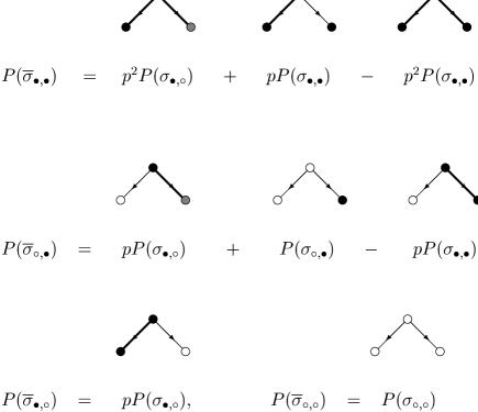
Figure 3: Pictorial representation of the rules for updating boundary polynomials in the new algorithm.

In Fig. 3 I have given a pictorial representation of how the boundary line polynomials are updated by the new algorithm. First it should be noted that there are two states per site with the following prescription: $\sigma_{i}=1$ if a bond has been inserted along an edge from the row above, and $\sigma_{i}=0$ otherwise. We are looking at a move similar to that in Fig. 1, though in this case the sites involved in the move are the one on the top and its neighbours in the row below. I shall refer to the configuration after the move as the ‘target’ configuration and it accounts for the state of the sites on the bottom row. The configurations prior to the move, given by the state of the top and bottom right sites, shall be called ‘source’ states. The state of sites away from the kink in the boundary does not influence the updating. In Fig. 3 sites with incoming bonds are marked with a filled circle, those with open circles have no incoming bonds, sites marked by a shaded circle have incoming bonds in the target state but not in the source state, and bonds are marked by thick lines. Note that the avoidance of dangling ends is easily achieved by ensuring that sites with incoming bonds have at least one outgoing bond. In the first equation the target configuration, $\overline{\sigma}_{\bullet,\bullet}$, has bonds entering both sites and is fed by the source configurations $\sigma_{\bullet,\circ}$ and $\sigma_{\bullet,\bullet}$. In moving the boundary from the top site, bonds can be inserted to the left and/or right. The source state $\sigma_{\bullet,\circ}$ has no bonds entering the left site so both bonds have to be added with an associated weight $p^{2}$. From the source state $\sigma_{\bullet,\bullet}$ a bond has to be inserted on the left edge, but on the right edge a bond can be either absent, in which case an associated weight $p$ is required, or a bond can be added giving a weight $-p^{2}$ because two bonds were inserted and two paths join on the site to the right. Similar considerations lead to the other equations.

Limiting the calculation to non-nodal contributions is very simple; whenever the boundary line reaches the horizontal position all one need do is set to zero the polynomials of states with a single incoming bond, i.e., states represented by integers of the form $2^{k}$. This obviously ensures that configurations with a nodal point are deleted from the calculation. The pair-connectedness at the following time can be calculated from the states with incoming bonds at nearest neighbour sites and no incoming bonds on any other sites.

In a calculation to a given order $n$ we need to calculate the non-nodal contributions for all $t\leq t_{\rm max}=n/2$. For a given $t^{\prime}<t$ the possible configurations along the boundary line is limited by constraints arising from the facts that graphs have to terminate at level $t$ and have no dangling parts. As mentioned, the “no dangling parts” restraint is equivalent to demanding that sites with incoming bonds also have outgoing bonds. Therefore a configuration for which the maximal separation between sites with incoming bonds is $r$ will take at least another $r-1$ steps before collapsing to a configuration with a pair of nearest neighbour sites with incoming bonds. Consequently if $t^{\prime}+r>t$ that configuration makes no contribution to $C(x,t)$ for any $x$ and can be discarded. Furthermore the minimum number of bonds needed to build up the internal structure of the configuration (that is the occupied sites except for the left- and right-most sites) will have to be inserted during the collapse of the configuration. Since we are interested only in non-nodal graphs we further know that we have to insert at least $2t$ bonds to get from the origin to a point $(x,t)$. It is easy to calculate the minimum order, $N_{\rm min}$, of the boundary polynomial as the configuration is built up, but in so doing we have also counted $2t^{\prime}$ bonds coming from the paths leading to the left- and right-most sites, respectively. So the minimal order to which a configuration contributes, $N_{\rm cont}$, from row $t^{\prime}$ is

$$N_{\rm cont}=2N_{\rm min}+2t-4t^{\prime}.$$ (11)

If $N_{\rm cont}>n$ the configuration can be discarded since it will only contribute at an order exceeding that to which we want to carry out our calculation. Further memory savings are obtained by observing that in calculating $C(x,t)$ we know that the non-nodal graphs have at least $2t$ bonds, so we need only store $n-2t$ coefficients, and when the boundary is moved from one row to the next we discard the two lowest order terms in the boundary polynomials since they are all zero.

The algorithm for calculating the series for directed site percolation is very similar, but of course we have different rules for updating the boundary polynomials. Though it should be noted that the meaning of ‘0’s and ‘1’s in the encoding of configurations is changed slightly to signify unoccupied and occupied sites respectively. The updating rules are easy to derive from those for the bond problem. In fact all we need to do is take the rules depicted in Fig. 3 and wherever we have inserted a bond on the right to a site already occupied the weight associated with that possibility is simply divided by $p$ because in site percolation we cannot reoccupy a site already occupied. This leads to the following update rules for the site problem:

$$P({\overline{\sigma}}_{\bullet,\bullet}) = p^{2}P(\sigma_{\bullet,\circ}),$$

$$P({\overline{\sigma}}_{\circ,\bullet}) = pP(\sigma_{\bullet,\circ})+P(\sigma_{\circ,\bullet})-P(\sigma_{\bullet,\bullet}),$$

$$P({\overline{\sigma}}_{\bullet,\circ}) = pP(\sigma_{\bullet,\circ}),$$ (12)

$$P({\overline{\sigma}}_{\circ,\circ}) = P(\sigma_{\circ,\circ}).$$

The only other change is that the formula for the minimal order of a contributing configuration is changed a little, becoming

$$N_{\rm cont}=2N_{\rm min}+2t-N_{\rm occ}-4t^{\prime}$$ (13)

where we have subtracted the number of occupied sites, $N_{\rm occ}$, in the configuration (otherwise they would have been counted twice from the first factor).

In Fig. 4 I have plotted the number of distinct configurations which make a contribution in a calculation of the square lattice bond series to order $n$. As can be seen the numerical evidence clearly shows that the asymptotic growth in the number of configurations is exponential with a growth factor $\lambda\leq\sqrt[8]{2}$. As already noted, this is a very substantial improvement on the previous best algorithm which had a growth factor $\lambda=\sqrt[4]{2}$. In plain words this means that whenever computer memory is doubled one can derive an additional 8 terms with the new algorithm as compared to an additional 4 terms with the previous best algorithm. Using all the memory minimization tricks mentioned above it is possible to derive the series for moments of the pair-connectedness to order 171 with a maximum of approximately 5.5Gb of memory. The old algorithm would have required more than 250 000 times as much memory and even if the extension procedure was used to derive say the last 20 terms correctly more than 10 000 times as much memory would have been required. For directed site percolation the series has been derived to order 158 using similar computational resources.

Finally a few remarks of a more technical nature. The number of contributing configurations becomes very sparse in the total set of possible states along the boundary line and as is standard in such cases one uses a hash-addressing scheme [31]. It is probably also worth mentioning that since the update involves only two nearest neighbour sites and does not depend on the state of other sites along the boundary, this algorithm lends itself very naturally to parallel computing. Since the integer coefficients occurring in the series expansion become very large, the calculation was performed using modular arithmetic [32]. This involves performing the calculation modulo various prime numbers $p_{i}$ and then reconstructing the full integer coefficients at the end. In order to save memory I used primes of the form $p_{i}=2^{15}-r_{i}$ so that the residues of the coefficients in the polynomials can be stored using 16-bit integers. The Chinese remainder theorem ensures that any integer has a unique representation in terms of residues. If the largest absolute values occurring in the final expansion is $m$, then we have to use a number of primes $k$ such that $p_{1}p_{2}\cdots p_{k}/2>m$. Note that it is not necessary to be able to uniquely reproduce the intermediate values, which in some cases can be much larger than the final ones. Up to 12 primes were needed to represent the coefficients correctly.

The updating rules given above are quite general and can be used for calculating the pair-connectedness of percolation problems on the directed square lattice in many other cases. One example is that of a lattice with an impenetrable wall [30], as shall be demonstrated in a forthcoming article, though in this case the calculation is not confined to non-nodal graphs. Other applications include directed percolation with temporal or spatial disorder in which the branching probability $p$ depends on $t$ or $x$ [33]. The basis for the algorithm used in this paper is Eq. (5). It is a very general expression for the pair connectedness which in fact should hold on any directed lattice and also for more complicated processes. Thus the work started in this paper can be generalized to other planar lattices or to higher dimensional lattices, though naturally the updating rules and other details of the actual implementation will vary from application to application. Another very interesting possibility is the application to unidirectionally coupled directed percolation [34, 35, 36]. In this case one studies a hierarchy of identical directed percolation processes. The 0’th level process is just an ordinary directed percolation process. The $k$’th level process is a directed percolation process evolving according to the usual rules. But in addition sites $(x,t)$ may become occupied at some given rate if the corresponding site was occupied at level $(k-1)$. Studies of this system showed that the exponents depend on $k$, in essence showing that as $k$ is increased percolation becomes easier. By truncating the hierarchy at some low value of $k$ it should be possible to generalize the algorithm to study this new and very interesting problem.

4 Analysis of series

The series for moments of the pair-connectedness were analyzed using differential approximants. A comprehensive review of these and other techniques for series analysis may be found in [20]. This allows one to locate the critical point and estimate the associated critical exponents fairly accurately, even in cases where there are additional non-physical singularities. Here it suffices to say that a $K$th-order differential approximant to a function $f$, for which one has derived a series expansion, is formed by matching the coefficients in the polynomials $Q_{i}$ and $P$ of order $N_{i}$ and $L$, respective, so that the solution to the inhomogeneous differential equation

$$\sum_{i=0}^{K}Q_{i}(x)(x\frac{\mbox{d}}{\mbox{d}x})^{i}\tilde{f}(x)=P(x)$$ (14)

agrees with the first series coefficients of $f$. The equations are readily solved as long as the total number of unknown coefficients in the polynomials is smaller than the order of the series $n$. The possible singularities of the series appear as the zeros $x_{i}$ of the polynomial $Q_{K}$ and the associated critical exponent $\lambda_{i}$ is estimated from the indicial equation

$$\lambda_{i}=K-1-\frac{Q_{K-1}(x_{i})}{x_{i}Q_{K}^{\prime}(x_{i})}.$$

The physical critical point is generally the first singularity on the positive real axis.

4.1 The bond series

In this section I will give a detailed account of the results of the analysis of the square bond series. The analysis of the square site is described in the following section. In addition to the moment series I have also analyzed the series $\mu_{0,2}(p)/\mu_{0,1}(p)\sim(p_{c}-p)^{-\nu_{\parallel}}$ and $\mu_{2,0}(p)\mu_{0,2}(p)/(\mu_{0,1}(p))^{2}\sim(p_{c}-p)^{-2\nu_{\perp}}$.

As one increases the order $N_{i}$ and $L$ of the polynomials in Eq. 14 and thus the number of terms used to form the differential approximants, one would generally expect to obtain more accurate estimates for the critical parameters. Likewise one often finds that the estimates show some dependence on the order $K$ of the differential approximant and/or the order $L$ of the inhomogeneous polynomial. In previous work [27] it was observed that for some series the estimates from first-order differential approximants showed a marked change with increasing $L$. Analysis of the longer series of course confirm this and also that some series (in particular $\mu_{0,1}(p)$ and $\mu_{0,2}(p)$) show a certain drift as $K$ is increased. But over all the estimates from the various series are exceptionally well converged and for $K\geq 2$ show little if any change as $L$ is changed or $K$ increased.

In order to gauge the effect of any systematic drift and lack of convergence to the true critical values it is helpful to plot the estimates of $p_{c}$ and associated exponents obtained from approximants to the various series as a function of the number of terms. Plotted in Fig. 5 are estimates for $p_{c}$ obtained from third-order differential approximants with $L$ increasing from 0 to 50 in steps of 5. The orders $N_{i}$ were chosen so that the difference between the order of the polynomials $Q_{i}$ never exceeded 1. Each point in the figure represents an estimate from a single approximant. From this study, two conclusions are immediately obvious. First of all most of the series show some drift in the estimate for $p_{c}$. In particular one notes that the estimates obtained from $\mu_{0,1}(p)$ and $\mu_{0,2}(p)$ (shown in the upper two panels on the right) do not appear to have converged yet. The estimates from the remaining series largely seem to have converged to a narrow band as the number of terms exceed 150. Secondly it appears that generally the scatter among the various estimates becomes smaller as the number of terms increases. All in all it appears that the estimates converge towards $p_{c}\simeq 0.644700185$. The only notable exception is perhaps the estimates from the series $\mu_{2,0}(p)\mu_{0,2}(p)/(\mu_{0,1}(p))^{2}$ (shown in the lower left panel) which seems to favor a slightly larger value $p_{c}\simeq 0.644700191$, though in this case there still seems to be a downwards trend in the estimates. It seems reasonable to estimate that $p_{c}=0.644700185(5)$. This is in good agreement with the estimate $p_{c}=0.64470015(5)$ obtained previously [27]. The new refined estimate is an order of magnitude more accurate and the central estimate lies within the error bounds of the earlier estimate. In Fig. 6 I have plotted estimates for the corresponding critical exponents. Similar trends are apparent in this case. From these plots I venture the following estimates

$$\gamma = 2.277730(5),$$

$$\nu_{\parallel} = 1.733847(6),$$

$$2\nu_{\perp} = 2.193708(4),$$

$$\gamma+\nu_{\parallel} = 4.01156(1),$$ (15)

$$\gamma+2\nu_{\parallel} = 5.74539(1),$$

$$\gamma+2\nu_{\perp} = 4.471425(15).$$

These estimates are again in full agreement with those obtained previously, an order of magnitude or so more accurate, and while the central estimates again are trending higher they still lie well within the earlier error bounds. Looking at differential approximants of different order (second and fourth) confirms the validity of these estimates.

I also analysed the series in order to estimate the leading confluent exponents $\Delta_{1}$. As was the case for the percolation probability series both the Baker-Hunter transformation and the method of Adler, Moshe and Privman (see [37] and references therein for details regarding these methods) yielded estimates consistent with $\Delta_{1}=1$. So there are no signs of non-analytic corrections to scaling.

4.2 The site series

An analysis similar to that of the previous section was performed for the site series. Generally I found that the estimates for $p_{c}$ were not so well converged. They seemed to change quite a bit as the order of the approximant or inhomogeneous polynomial increased, and furthermore the estimates also showed some inconsistencies from series to series. The series for $\mu_{0,2}(p)$ and $\mu_{0,1}(p)$ yielded estimates for $p_{c}\simeq 0.7054850$ while the series $\mu_{2,0}(p)\mu_{0,2}(p)/(\mu_{0,1}(p))^{2}$ favored an estimate $p_{c}\simeq 0.7054853$ with the remaining series yielding estimates in between. From these one could surmise that $p_{c}=0.70548515(20)$. The associated estimate for the critical exponents are listed below

$$\gamma = 2.27765(6),$$

$$\nu_{\parallel} = 1.73381(4),$$

$$2\nu_{\perp} = 2.19377(5),$$

$$\gamma+\nu_{\parallel} = 4.01135(15),$$ (16)

$$\gamma+2\nu_{\parallel} = 5.7450(2),$$

$$\gamma+2\nu_{\perp} = 4.47130(8).$$

As can be seen these estimates are often only marginally consistent with those from the bond series and at least an order of magnitude less accurate.

Due to the high degree of internal consistency of the estimates from the bond series one would tend to believe quite firmly in their accuracy and correctness and one can then use them to try and obtain a more accurate estimate for $p_{c}$ in the site problem. In Fig. 7 I have plotted the estimates for the critical exponents vs the estimates for $p_{c}$. The solid lines indicate the error-bounds on the exponent estimates obtained by using the bond-series estimates for the exponents $\gamma$, $\nu_{\parallel}$ and $\nu_{\perp}$. By extrapolating the exponent estimates until they lie between the solid lines it is obvious that this procedure yields a $p_{c}$ estimate consistent with $p_{c}=0.70548522(4)$, which I take as the final estimate.

4.3 Non-physical singularities

Non-physical singularities are of interest both because knowlegde about their position and associated exponents may help in the search for exact solutions and because one may gain a better understanding of the problem by studying the behaviour of various physical quantities as analytic functions of complex variables. While comparatively little work has been done along these lines for directed percolation this is a quite active field of study for classical spin systems such as the Potts and Ising models (see [38] for recent results and references to earlier work) .

The series have a radius of convergence smaller than $p_{c}$ due to singularities in the complex $p$-plane closer to the origin than the physical critical point. Since all the coefficients in the expansion are real, complex singularities always come in conjugate pairs. In order to locate the non-physical singularities in a systematic fashion I used the following procedure: Calculate all differential approximants with $K$ and $L$ fixed using at least 150 or 140 terms in the bond or site cases, respectively. Each approximant yields $N_{K}$ possible singularities (and associated exponents) from the zeros of $Q_{K}$ (many of these are of course not actual singularities of the series). Next sort these ‘singularities’ into equivalence classes by the criterion that they lie at most a distance $2^{-k}$ apart. An equivalence class is accepted as a singularity if it contains more than $N_{a}$ approximants ($N_{a}$ can be adjusted but I typically used a value around 2/3 of the total number of approximants), and an estimate for the singularity and exponent is obtained by averaging over the approximants (the spread among the approximants is also calculated). This calculation was then repeated for $k-1$, $k-2$, $\ldots$ until a minimal value of 6. To avoid outputting well converged singularities at every level, once an equivalence class has been accepted, the approximants which are members of it are removed, and the subsequent analysis is carried out only on the remaining data. This procedure is applied to each series in turn, producing tables of possible singularities.

The analysis indicates that the series have quite a large number of non-physical singularities. A quick view of the distribution of singularities can be gained from Fig. 8 which show the location of the non-physical singularities. Estimates for the non-physical singularities are listed in Table 1. For both the bond and site cases there are two sets of singularities. For those marked by 1, quite accurate estimates can be obtained for both the location of the singularity and the associated exponents. The exponent estimates for the site problem at the singularity on the negative axis are consistent with the exact values 1/2, $-1/2$, $-3/2$, and $-1/2$ for the series $S(p)$, $\mu_{0,1}$, $\mu_{0,2}$, and $\mu_{2,0}$, respectively. At the conjugate pair of complex singularities the corresponding exponents are consistent with the exact values 3, 2, 1 and 2, respectively. In either case the error is no more than 0.1%. In the bond case the exponents at the conjugate pair of complex singularities seem to be identical to those for the site problem though the error is at least an order of magnitude larger. At the singularity on negative axis the exponent estimates are $-0.075(5)$, $-1.05(2)$, $-2.025(15)$, and $-1.00(2)$. So the most likely scenario for exact values would seem to be a logarithmic divergence in S(p), and divergences with exponents $-1$, $-2$, and $-1$ in $\mu_{0,1}$, $\mu_{0,2}$, and $\mu_{2,0}$, respectively. For the singularities marked 2, the estimates for the location of the singularity is poor and no meaningful estimates can be obtained for the exponents. In all cases the singularities are found in all series and remain fairly stable as $K$ and $L$ is varied.

5 Conclusion

In this paper I have reported on a new algorithm for the derivation of low-density series for moments of the pair-connectedness in directed percolation problems. Numerical evidence shows that the computational complexity grows exponentially, but with a growth factor $\lambda<\sqrt[8]{2}$, which is much smaller than the growth factor $\lambda=\sqrt[4]{2}$ of the previous best algorithm. For bond (site) percolation on the directed square lattice the series have been extended to order 171 (158) as compared to order 112 (106) obtained in previous work [27].

Analysis of the bond series led to a very accurate estimate for the critical point, $p_{c}=0.644700185(5)$, and the values of the critical exponents for the average cluster size, parallel and perpendicular connectedness lengths are estimated to be $\gamma=2.277730(5)$, $\nu_{\parallel}=1.733847(6)$ and $\nu_{\perp}=1.096854(4)$. An accurate estimate for the percolation probability exponent is obtained from the scaling relation $\beta=(\nu_{\parallel}+\nu_{\perp}-\gamma)/2=0.276486(8)$.

For reference purposes I list estimates for some other critical exponents obtained using various scaling relations:

$$\Delta= \beta+\gamma= 2.554216(13)$$

$$\tau= \nu_{\parallel}-\beta= 1.457362(14)$$

$$z= \nu_{\parallel}/\nu_{\perp}= 1.580745(10)$$

$$\gamma^{\prime}= \gamma-\nu_{\parallel}= 0.543883(11)$$

$$\delta= \beta/\nu_{\parallel}= 0.159464(6)$$

$$\eta= \gamma/\nu_{\parallel}-1= 0.313686(8).$$

Here $\Delta$ is the exponent characterizing the scale of the cluster size distribution, $\tau$ is the cluster length exponent, $z$ is the dynamical critical exponent, $\gamma^{\prime}$ the exponent characterizing the steady-state fluctuations of the order parameter, while $\delta$ and $\eta$ characterize the behaviour at $p_{c}$ as $t\rightarrow\infty$ of the survival probability and average number of particles, respectively.

Assuming that the exponent estimates from the square bond case are correct, an improved $p_{c}$-estimate was obtained for the square site problem, $p_{c}=0.70548522(4)$.

Finally I note, that an analysis of the series, in order to determine the value of the confluent exponent, yielded estimates consistent with $\Delta_{1}\simeq 1$. Thus there is no evidence of non-analytic corrections to scaling.

E-mail or WWW retrieval of series

The series for the directed percolation problems on the various lattices can be obtained via e-mail by sending a request to I.Jensen@ms.unimelb.edu.au or via the world wide web on the URL http://www.ms.unimelb.edu.au/~iwan/ by following the instructions.

Table 1: Estimates of the location of various non-physical singularities in the series for directed bond and site percolation.

	Bond	Site
1	$-0.51670(3)$	$-0.451952165(8)$
1	$-0.22605(10)\pm 0.4400(1)i$	$-0.2661783(4)\pm 0.3847813(4)i$
2	$0.135(10)\pm 0.455(10)i$	$-0.0525(5)\pm 0.4840(5)i$
2	$0.0105(10)\pm 0.475(1)i$	$0.085(15)\pm 0.500(15)i$

Figure 2: Illustration of graphs which contribute to $C(x,t)$ (solid lines), $C(x^{\prime},t^{\prime})$ (solid+dashed lines) and paths which are not allowed (dotted lines).

Figure 4: The maximal number of contributing configurations in a calculation to order $N$. The straight line is a pure exponential $\propto\lambda^{N}$ with growth factor $\lambda={\sqrt[8]{2}}$.

Figure 5: Estimates of the critical point $p_{c}$ obtained from third-order differential approximants vs the number of terms used by the approximant. Numbers along the $y$-axis are all preceded by 0.644700. Shown are (from left to right and top to bottom) estimates from the series $S(p)$, $\mu_{0,1}(p)$, $\mu_{2,0}(p)$, $\mu_{0,2}(p)$, $\mu_{2,0}(p)\mu_{0,2}(p)/(\mu_{0,1}(p))^{2}$, and $\mu_{0,2}(p)/\mu_{0,1}(p)$.

Figure 6: Estimates of the critical exponents obtained from third-order differential approximants vs the number of terms used by the approximant. Shown are (from left to right and top to bottom) estimates from the series $S(p)$, $\mu_{0,1}(p)$, $\mu_{2,0}(p)$, $\mu_{0,2}(p)$, $\mu_{2,0}(p)\mu_{0,2}(p)/(\mu_{0,1}(p))^{2}$, and $\mu_{0,2}(p)/\mu_{0,1}(p)$.

Figure 7: Estimates of the critical exponents obtained from third-order differential approximants vs estimates of the critical point for square site problem. Numbers along the $x$-axis are all preceded by 0.70548. Shown are (from left to right and top to bottom) estimates from the series $S(p)$, $\mu_{0,1}(p)$, $\mu_{2,0}(p)$, $\mu_{0,2}(p)$, $\mu_{2,0}(p)\mu_{0,2}(p)/(\mu_{0,1}(p))^{2}$, and $\mu_{0,2}(p)/\mu_{0,1}(p)$.

Figure 8: Location of non-physical singularities for bond (left panel) and site (right panel) directed percolation.

References

- [1] Percolation Structures and Processes, Ann. Israel Phys. Soc. 5, eds. G. Deutsher, R. Zallen, and J. Adler, Adam Hilger, Bristol, (1983).
- [2] D. Stauffer and A. Aharony, Introduction to Percolation Theory, 2. Edition, Taylor & Francis, London, (1992).
- [3] K. De’Bell and J. W. Essam, J. Phys. A 14, 1993 (1981).
- [4] J. Kertész and T. Viscek, J. Phys. C 13, L343 (1980).
- [5] S. Redner and A. C. Brown, J. Phys. A 14, L285 (1981).
- [6] P. Grassberger and K. Sundermeyer, Phys. Lett. 77B, 220 (1978); J. L. Cardy and R. Sugar, J. Phys. A 13, L423 (1980).
- [7] F. Schlögl, Z. Phys 252, 147 (1972); P. Grassberger and A. de la Torre, Ann. Phys. (NY) 122, 373 (1979).
- [8] R. M. Ziff, E. Gulari, and Y. Barshad, Phys. Rev. Lett. 56, 2553 (1986); J. Köhler and D. ben-Avraham, J. Phys. A 24, L621 (1991); H. Takayasu and A. Y. Tretyakov, Phys. Rev. Lett. 68, 3060 (1992); I. Jensen, Phys. Rev. Lett. 70, 1465 (1993).
- [9] S. P. Obukhov, Phys. Rev. Lett. 65, 1395 (1990); M. Paczuski, S. Maslov and P. Bak, Europhys. Lett. 27, 97 (1994).
- [10] L. S. Schulman and P. E. Seiden, J. Stat. Phys. 27, 83 (1982).
- [11] E. Domany and W. Kinzel, Phys. Rev. Lett. 53, 311 (1984); W. Kinzel, Z. Phys. B 58, 229 (1985).
- [12] M. F. Sykes and J. W. Essam, J. Math. Phys. 5, 1117 (1964).
- [13] J. Cardy, in Phase Transitions and Critical Phenomena, Vol. 11, eds. C. Domb and J. L. Lebowitz, Academic Press, New York (1987).
- [14] F. Y. Wu, Rev. Mod. Phys. 54, 235 (1982).
- [15] C. M. Fortuin and P. W. Kasterleyn, Physica 57, 536 (1972).
- [16] J. W. Essam, J. Phys. A 22, 4927 (1989).
- [17] D. K. Arrowsmith and J. W. Essam, Phys. Rev. Lett. 65, 3068 (1990).
- [18] T. Tsuchiya and M. Katori, J. Phys. Soc. Jpn. 67, 1655 (1998).
- [19] J. Cardy and F. Colaiori, Phys. Rev. Lett. 82, 2232 (1999).
- [20] A. J. Guttmann, in Phase Transitions and Critical Phenomena, Vol. 13, eds. C. Domb and J. L. Lebowitz, Academic Press, New York (1989).
- [21] D. Dhar, M. H. Phani and M. Barma, J. Phys. A 15, L213 (1982).
- [22] J. Blease, J. Phys. A 10, 917 and 3461 (1977).
- [23] K. De’Bell and J. W. Essam, J. Phys. A 16, 385 (1983).
- [24] J. W. Essam, K. De’Bell, J. Adler and F. M. Bhatti, Phys. Rev. B 33, 1982 (1986).
- [25] J. W. Essam, A. J. Guttmann and K. De’Bell, J. Phys. A 21, 3815 (1988).
- [26] F. M. Bhatti and J. W. Essam, J. Phys. A 17, L67 (1984).
- [27] I. Jensen, J. Phys. A 29, 7013 (1996).
- [28] R. J. Baxter and A. J. Guttmann, J. Phys. A 21, 3193 (1988).
- [29] D. K. Arrowsmith and J. W. Essam, J. Math. Phys. 18, 235 (1977).
- [30] J. W. Essam, A. J. Guttmann, I. Jensen and D. TanlaKishani, J. Phys. A 29, 1619 (1996).
- [31] K. Mehlhorn, Data Structures and Algorithms I: Sorting and Searching, EATCS Monographs on Theoretical Computer Science, Springer-Verlag, Berlin (1984).
- [32] D. E. Knuth, Seminumerical Algorithms (The Art of Computer Programming 2), Addison-Wesley, Reading, MA (1969).
- [33] I. Jensen, Phys. Rev. Lett. 77, 4988 (1996).
- [34] U. C. Täuber, M. J. Howard and H. Hinrichsen, Phys. Rev Lett. 80, 2165 (1998).
- [35] Y. Y. Goldschmidt, H. Hinrichse , M. J. Howard and U. C. Täuber, preprint, cond-mat/9809166.
- [36] H. K. Janssen, preprint, cond-mat/9901188.
- [37] I. Jensen and A. J. Guttmann, J. Phys. A 28, 4813 (1995).
- [38] V. Matveev and R. Shrock, J. Phys. A 28, L533 (1995); Phys. Rev. E 54, 6174 (1996); H. Feldmann, R. Shrock andS.-H. Tsai, Phys. Rev. E 57, 1335 (1998).