Interplay of disorder and nonlinearity in Klein-Gordon models: Immobile kinks

Abstract

We consider Klein-Gordon models with a $\delta$-correlated spatial disorder. We show that the properties of immobile kinks exhibit strong dependence on the assumptions as to their statistical distribution over the minima of the effective random potential. Namely, there exists a crossover from monotonically increasing (when a kink occupies the deepest potential well) to the non-monotonic (at equiprobable distribution of kinks over the potential minima) dependence of the average kink width as a function of the disorder intensity. We show also that the same crossover may take place with changing size of the system.

I Introduction

An extensive research work on the static and transport properties of nonlinear excitations in various soliton-bearing disordered systems has been undertaken in the last decade (see Refs. [1] and [2]). It is well known that when taken separately both the nonlinearity and disorder contribute to the localization effects, the character of localization being however essentially different. The nonlinearity results in the possibility of existence of nonlinear localized excitations usually referred to as solitons that are rather robust and can propagate through the system undistortedly. At the same time the disorder (in linear systems) evokes the Anderson localization, which manifests itself in the behavior of the transmission coefficient of a plane wave decaying exponentially with the system width. These two localization mechanisms are competitive to some extent; taken together, the nonlinearity and disorder may lead to a number of qualitatively new effects, namely, the transmission coefficient tending to zero with increasing the system length according to a power law [3, 4] rather than exponentially (which would be otherwise the property of a linear system); there can arise a multistability [3, 4, 5] in the wave transmission through a disordered slab; excitations in highly nonlinear or multidimensional nonlinear Schrödinger (NLS) systems (which would either disperse or collapse otherwise) can be stabilized by disorder. [6, 7, 8]

In the present paper we study the static properties of a one-kink solution (or, equivalently, of a diluted kink gas) of disordered Klein-Gordon models where the disorder is assumed to be a $\delta$-correlated Gaussian spatial noise. The disorder of the kind is akin, for example, to Josephson junctions, where it is caused by the fluctuations of the gap between two superconductor plates. Quite recently Mints proposed [9] a similar model with randomly alternating critical current density to account for a self-generated magnetic flux observed [10] experimentally. We discuss his results in more detail in the Conclusion.

In general, Klein-Gordon models have been repeatedly studied [1, 2, 11] for the disorder represented by a lattice of $\delta$-like impurity potentials with random positions of the impurities and either equal or randomly distributed intensities. It was found out that in a number of cases the kink dynamics in disordered systems could be adequately described within the framework of the collective coordinates approach (Refs. [12, 13, 14, 15], and references therein). This is the background of our restricting ourselves to the said approach in the scope of the present paper providing however at each step the validation of analytical results comparing them to the numerical simulations of the original system. We emphasize that in opposite to, for example, Refs. [2] and [11], we use Rice’s collective coordinates approach [16, 17] with the kink width being the variational parameter.

A similar approach has been recently applied for two other one-dimensional (1D) systems: Bussac et al. investigated [6] the effects of the polaron ground state in a deformable chain, while Christiansen et al. considered [7] the stabilization of nonlinear excitations by disorder in the NLS model. It should be indicated that investigation of these two (in fact closely related) systems leads to one and the same result: the width of stationary solitons decreases with growing intensity of the disorder. The importance of this conclusion resides in its prediction that the disorder can stabilize otherwise unstable solitons in 2D and 3D NLS models. Quite recently this prediction was borne out numerically [8] for the 2D case. It must be emphasized that for NLS models the conclusion does not depend on the averaging procedure: one can equally perform averaging either on absolute ground states [6] or over all local minima of the effective random potential with equal weights. [7, 8] We show that it is not the case for the Klein-Gordon models: their properties exhibit strong dependence on the assumptions as to the statistical distribution of kinks over the minima of the effective random potential. For the purely dynamical problem these statistics are left beyond consideration and should be thus imposed as an additional assumption. We use Jaynes’s maximum entropy inference [18] for this purpose.

The outline of the paper is the following. In Sec. II we present the model and derive the equations for the collective coordinates of the kink taking into account the disorder via the effective random potential. In Sec. III we investigate both analytically and numerically the case of immobile kinks and demonstrate the existence of the crossover between monotonic and nonmonotonic dependence of the average kink width as a function of the disorder intensity. In Sec. IV we summarize the exposed results.

II Collective coordinates approach

We consider a Klein-Gordon (KG) model in the presence of space disorder. The Hamiltonian of the system has the form

$$H=\int_{-\infty}^{\infty}dx\biggl{\{}\frac{1}{2}(\phi_{t}^{2}+\phi_{x}^{2})+[1-\eta\epsilon(x)]\Phi(\phi)\biggr{\}}\;,$$ (1)

where the subscripts stand for partial derivatives with respect to the indicated variables and units are chosen so that the Hamiltonian is already in the scaled form. The potential $\Phi(\phi)$ has the form

$$\Phi(\phi)=1-\cos\phi$$ (2)

for the sine-Gordon (SG) model, and

$$\Phi(\phi)=\frac{1}{4}(\phi^{2}-1)^{2}$$ (3)

for the $\phi^{4}$ model. We assume that $\epsilon(x)$ is delta-correlated spatial disorder

$$\langle\epsilon(x)\epsilon(x^{\prime})\rangle=\delta(x-x^{\prime})\;,$$ (4)

(the brackets $\langle...\rangle$ denote averaging over all realizations of the disorder) with the Gaussian distribution

$$p[\epsilon(x)]=\frac{1}{\sqrt{\pi}}\exp[-\epsilon^{2}(x)]\;.$$ (5)

We have studied both SG (2) and $\phi^{4}$ (3) models. Although properties of these two models show many similarities, they also exhibit a number of interesting distinctions related, in particular, to the existence of a breather state in the SG model and of Rice’s internal mode [16, 17] in the $\phi^{4}$ model. So, it was important to compare the effects of disorder in both these models. But since the qualitative features of the exposed models turned out to coincide in the scope of our present investigations, we dare not overload the paper with unnecessary repetitions and restrict ourselves with presenting in detail the sine-Gordon model only, keeping in mind although that every stage of the calculations applies for the $\phi^{4}$ model as well.

The SG system is governed by the equation of motion

$$\phi_{tt}-\phi_{xx}+[1-\eta\epsilon(x)]\sin\phi+\gamma\phi_{t}=0\;,$$ (6)

where the damping term with the damping constant $\gamma$ has been included. It is well known that in the absence of disorder and damping ($\eta=\gamma=0$) Eq. (6) is completely integrable and possesses a topologically stable solution in the form of a kink given by

$$\phi_{K}(x,t)=4\arctan\exp\biggl{(}\frac{x-X(t)}{L(t)}\biggr{)}\;,$$ (7)

where $X(t)=X_{0}+vt$ is the kink coordinate, $v$ is its velocity, and $L=\sqrt{1-v^{2}}$ is the kink width.

In the general case of Eq. (6) for a number of situations the kink emission is exponentially small, [14] so that the kink dynamics can be studied by the collective coordinate approach. In the framework of this approach the variables $X(t)$ and $L(t)$ are understood as time-dependent variational parameters. Inserting Eq. (7) into Hamiltonian (1) as a trial function, we obtain the effective Hamiltonian

$$H_{eff}=\frac{L}{16}p_{X}^{2}+\frac{3L}{4\pi^{2}}p_{L}^{2}+U(L)+V(\{\epsilon\},L,X)\;,$$ (8)

with momenta

$$p_{X}=\frac{8}{L}\frac{dX}{dt}\;,\qquad p_{L}=\frac{2\pi^{2}}{3L}\frac{dL}{dt}\;.$$ (9)

Here

$$U(L)=\frac{4}{L}+4L\;$$ (10)

is the potential function in the case of no disorder and

$$V(\{\epsilon\},L,X)=-2\eta\int_{-\infty}^{\infty}dx\epsilon(x)\;\mbox{sech}^{2}\biggl{(}\frac{x-X}{L}\biggr{)}$$ (11)

is the effective random potential arising because of the disorder term. Then, taking into account the damping, we arrive at the following equations of motion: [16]

$$\frac{dp_{X}}{dt}+\gamma p_{X}+\frac{d}{dX}V(\{\epsilon\},L,X)=0\;,$$ (12)

$$\frac{dp_{L}}{dt} + \gamma p_{L}+\frac{3p_{L}^{2}}{4\pi^{2}}+\frac{p_{X}^{2}}{16}$$ (13)

$$+ \frac{d}{dL}[U(L)+V(\{\epsilon\},L,X)]=0\;.$$ (14)

In the following section we solve approximately these equations of motion for immobile kinks and compare the results to the results of direct numerical integration of Eq. (6).

III Results for immobile kinks

As a consequence of the damping $\gamma$ the kink will eventually stop at some stable or metastable stationary position along the system. Here we do not consider this transient stage and assume that the kink is already immobile [$dp_{L}/dt=p_{L}=p_{X}=0$]. In this case the equations of motion (12) and (13) take on the form

$$\frac{d}{dX}V(\{\epsilon\},L,X)=0\;,$$ (15)

$$\frac{d}{dL}[U(L)+V(\{\epsilon\},L,X)]=0\;.$$ (16)

Considering the center-of-mass motion described by Eq. (12) we observe that for each realization of the random potential $\epsilon(x)$ the stable stationary position $X=X_{m}(\{\epsilon\},L)$ of the kink is defined by the point where $V(\{\epsilon\},L,X)$ has a minimum with respect to $X$. Thus we can now insert the value $X=X_{m}(\{\epsilon\},L)$ into Eq. (16) and, solving the resulting equation

$$L=\biggl{(}1+\frac{1}{4}\frac{d}{dL}V(\{\epsilon\},L,X_{m})\biggr{)}^{-1/2}\;,$$ (17)

get the value of the stationary kink width $L(\{\epsilon\})$ at given position of the kink. Encountering a similar problem for the case of NLS system, Christiansen et al. invoked [7] the mean-field approximation

$$\langle\frac{d}{dL}V(\{\epsilon\},L,X_{m})\rangle\approx\frac{d}{dL}\langle V(\{\epsilon\},L,X_{m})\rangle\;.$$ (18)

Further the estimation of the quantity $\langle V\rangle$ was performed using Rice’s averaging theorem. [19, 20] However, being rather good for the NLS model [7] the mean-field approximation (18) fails for the KG models. Thereby we were forced to use a more precise averaging procedure calculating $\langle dV/dL\rangle$ directly.

Expanding Eq. (17) into series up to the second order in $\eta$,

$$L\approx 1-\frac{1}{8}\frac{dV}{dL}+\frac{3}{128}\biggl{(}\frac{dV}{dL}\biggr{)}^{2}\;,$$ (19)

and solving by iterations we get after averaging [which by means of Eq. (4) can be performed for the terms containing $\eta^{2}$ exactly] the average kink width

$$L_{var}\equiv\langle L(\{\epsilon\})\rangle\approx 1+\frac{\eta}{2}\langle\lambda(\{\epsilon\},X_{m})\rangle+\frac{\pi^{2}}{180}\,\eta^{2}\;,$$ (20)

where the averaging of the function

$$\lambda(\{\epsilon\},X)=\int_{-\infty}^{\infty}dx\epsilon(x)(x-X)\frac{\sinh(x-X)}{\cosh^{3}(x-X)}\;$$ (21)

is performed over all realizations of the disorder in the points $X=X_{m}$ in which the potential

$$V(\{\epsilon\},L,X)\approx 2\eta\mu(\{\epsilon\},X)\;$$ (22)

with

$$\mu(\{\epsilon\},X)=-\int_{-\infty}^{\infty}dx\epsilon(x)\mbox{sech}^{2}(x-X)\;$$ (23)

takes on its minima on $X$.

Thus we arrive at the problem of performing the average of $\lambda(\{\epsilon\},X_{m})$ over the minima $X_{m}$ of the function $\mu(\{\epsilon\},X)$. It is convenient for later use to perform this averaging in two steps calculating at the outset

$$\Lambda(\tilde{\mu})=\int_{-\infty}^{\infty}\tilde{\lambda}\,P_{l}(\tilde{\lambda}\mid\tilde{\mu})d\tilde{\lambda}\;$$ (24)

and thereafter

$$\langle\lambda(\{\epsilon\},X_{m})\rangle=\int_{-\infty}^{\infty}\Lambda(\tilde{\mu})P_{m}(\tilde{\mu})d\tilde{\mu}\;.$$ (25)

Here $P_{l}(\tilde{\lambda}\mid\tilde{\mu})$ is the conditional probability that $\lambda(\{\epsilon\},X_{m})$ has the value $\tilde{\lambda}$ if $\mu(\{\epsilon\},X_{m})$ equals to $\tilde{\mu}$. Correspondingly, $\Lambda(\tilde{\mu})$ is the value of $\lambda(\{\epsilon\},X_{m})$ averaged over all realizations of the disorder for which $\mu(\{\epsilon\},X_{m})$ is equal to $\tilde{\mu}$. It is difficult to calculate $\Lambda(\tilde{\mu})$ analytically but numerical simulations show (see Fig. 1) that up to very good accuracy the dependence $\Lambda(\tilde{\mu})$ is linear:

$$\Lambda(\tilde{\mu})\simeq-0.344\,\tilde{\mu}-0.500\;.$$ (26)

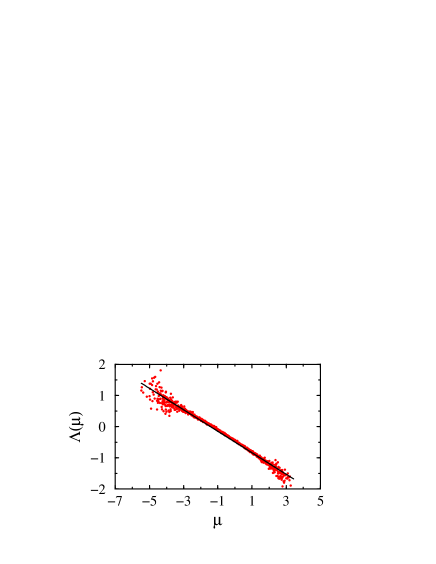
FIG. 1.: The dependence $\Lambda(\tilde{\mu})$ found numerically. The calculations are performed for a million minima of the function $\mu(\{\epsilon\},X)$.

Substituting it into Eq. (25) we obtain that

$$\langle\lambda(\{\epsilon\},X_{m})\rangle\simeq-0.344\,\langle\mu(\{\epsilon\},X_{m})\rangle-0.500\;,$$ (27)

where

$$\langle\mu(\{\epsilon\},X_{m})\rangle=\int_{-\infty}^{\infty}\tilde{\mu}\,P_{m}(\tilde{\mu})d\tilde{\mu}\;$$ (28)

is the average value of the function $\mu(\{\epsilon\},X)$ over its minima $X_{m}$. Here the probability density $P_{m}(\tilde{\mu})$ is a product of two factors. The first one is the probability density that some arbitrary chosen minimum $X_{m}$ of the function $\mu(\{\epsilon\},X)$ will be equal to $\tilde{\mu}$. We denote this probability density as $p_{min}(\tilde{\mu})$. The second factor is the conditional probability that if the minimum is equal to $\tilde{\mu}$ it will be actually occupied by the kink. It is evident that in a real system the kink is more likely to occupy the deeper minimum than the shallow one. So to be consequential one must ascribe to every minimum of the function $\mu(\{\epsilon\},X)$ some probability weight and average taking into account those probabilities. But the values of these probabilities are in general determined by the whole prehistory of the kink. These values are not contained in the dynamical equations of motion that state only that the kink should take on some minimum regardless to its depth. It would be a cumbersome problem to calculate them appropriately. That is why two limit cases are in general considered: either the kink seats itself into the deepest well [6] or it rather occupies any of them with equal probabilities. [7] As it was already remarked in the Introduction, both limit cases lead to qualitatively the same results for the NLS model.

It is not the case of KG models where, as it will be shown later, different assumptions as to the a priori weights of minima lead to qualitatively different behavior of the kink width. Since we are merely lacking information sufficient enough to reconstruct these weights in an objectivistic fashion, a remedy would be Jaynes’s maximum entropy inference, [18] according to which the simplest self-consistent unbiased choice is to assume that the kink will occupy a potential well corresponding to the minimum $X_{m}$ of the function $\mu(\{\epsilon\},X)$ [for given profile $\epsilon(x)$] with probability proportional to $e^{-\beta\mu(\{\epsilon\},X_{m})}$ thus introducing an additional parameter $\beta$ (following Jaynes we shall call it a conjugate parameter). By this expedience we present some natural interpolation covering two mentioned limit cases: of equiprobable distribution ($\beta=0$) and of averaging over the deepest minima only ($\beta\to\infty$). So we can write

$$P_{m}(\tilde{\mu})=\frac{1}{{\cal Z}}e^{-\beta\tilde{\mu}}p_{min}(\tilde{\mu})\;,$$ (29)

where

$${\cal Z}(\beta)=\int_{-\infty}^{\infty}d\tilde{\mu}e^{-\beta\tilde{\mu}}p_{min}(\tilde{\mu})\;$$ (30)

plays part of the partition function.

To calculate $p_{min}(\tilde{\mu})$ we follow Ref. [7] and make use of the Rice’s averaging theorem [19, 20] [valid for the case, well attested by the numerics, of $\mu(\{\epsilon\},X)$ being a stationary centered Gaussian process] stating that the probability density of some given minimum of the function $\mu(\{\epsilon\},X)$ to be equal to $\tilde{\mu}$ is

$$p_{min}(\tilde{\mu})=\frac{1}{\sqrt{2\pi M_{0}}}\,\sigma\biggl{(}\frac{\tilde{\mu}}{\sqrt{2M_{0}}}\,,\,\sqrt{1-\frac{M_{2}^{2}}{M_{0}M_{4}}}\biggr{)}\;,$$ (31)

where the function

$$\sigma(y,\kappa) = \kappa e^{-(y/\kappa)^{2}}$$ (32)

$$- 2\sqrt{1-\kappa^{2}}ye^{-y^{2}}\int_{(y/\kappa)\sqrt{1-\kappa^{2}}}^{\infty}e^{-t^{2}}dt\;,$$ (33)

and the spectral momenta

$$M_{0}=\langle[\mu(\{\epsilon\},X)]^{2}\rangle=\frac{4}{3}\;,$$ (34)

$$M_{2}=\langle[\mu_{X}(\{\epsilon\},X)]^{2}\rangle=\frac{16}{15}\;,$$ (35)

$$M_{4}=\langle[\mu_{XX}(\{\epsilon\},X)]^{2}\rangle=\frac{64}{21}\;,$$ (36)

were introduced.

Hence the partition function takes on the form

$${\cal Z}(\beta)=\frac{1}{\sqrt{\pi}}\int_{-\infty}^{\infty}dxe^{-\sqrt{8/3}\,\beta x}\sigma\left(x,\frac{3}{5}\sqrt{2}\right)$$ (37)

and can be expanded into series in $\beta$ yielding the average value

$$\langle\mu(\{\epsilon\},X_{m})\rangle=-\frac{d}{d\beta}\ln{\cal Z}(\beta)$$ (38)

$$=-\frac{1}{5}\sqrt{\frac{7\pi}{6}}-\frac{2}{75}(64-7\pi)\,\beta+{\cal O}(\beta^{2}).\;$$ (39)

And now, substituting it into Eqs. (27) and (20) we obtain for the average kink width

$$L_{var}\approx 1+(0.193\beta-0.059)\,\eta+\frac{\pi^{2}}{180}\,\eta^{2}\;.$$ (40)

Thus it is seen that there is a qualitative change of the kink width behavior as function of the disorder intensity $\eta$ according to whether the value of conjugate parameter $\beta$ is below or above some critical value $\beta_{cr}\approx 0.3$.

At small $\beta$ the average kink width is a nonmonotonic function of the disorder intensity $\eta$: it decreases at small intensities but starts to increase thereafter. This result is well attested by the direct numerical calculations of stationary kink solutions of the initial equation of motion (6). In Fig. 2 we compare the analytical prediction given by Eq. (40) with the numerical results for the case of equiprobable distribution of the kinks over the potential wells ($\beta=0$). The numerical results have been obtained as an average of 1000 realizations of the disorder. Two different expressions for the kink width were calculated:

$$L_{cos}=\frac{1}{4}\int_{-\infty}^{\infty}dx\{1-\cos[\phi(x)]\}\;,$$ (41)

and

$$L_{der}=8\biggl{\{}\int_{-\infty}^{\infty}dx\biggl{[}\frac{d\phi(x)}{dx}\biggr{]}^{2}\biggr{\}}^{-1}\;.$$ (42)

From the point of view of the collective coordinate approach $L_{cos}$ and $L_{der}$ should coincide with the value of $L$ introduced in Eq. (7). Indeed, as it is seen from the figures, it does take place for $0\leq\eta\lesssim 0.2$; thus, these are limits where the collective coordinate approach works well.

FIG. 2.: The dependence of the average (on 1000 realizations of the disorder) kink width $\langle L(\{\epsilon\})\rangle$ vs disorder intensity $\eta$ under the assumption that the kink occupies every potential well created by disorder with equal probability. The system length $R=15$.

FIG. 3.: The dependence of the average (on 1000 realizations of the disorder) kink width $\langle L(\{\epsilon\})\rangle$ vs disorder intensity $\eta$ under the assumption that the kink sits into the deepest potential well created by disorder. The system length $R=15$.

Going on with the analysis of Eq. (40) we see that at big values of the conjugate parameter ($\beta>\beta_{cr}$) when the kink rather occupies deep potential wells, the kink width should grow monotonically with the disorder. But it is evident that in this case the analytical approach discussed above is applicable to systems of infinite length only. For the finite system the case of big $\beta$ represents the situation when the kink sits in the deepest potential well. Obviously its average depth essentially depends on the system length. We can make an estimation of this dependence drawing on the formula [20] for the average number of minima of the function $\mu(\{\epsilon\},X)$ on an interval $R$ whose values lie below some $\tilde{\mu}$:

$$N_{min}=\frac{R}{2\pi}\sqrt{\frac{M_{2}}{M_{0}}}e^{-\tilde{\mu}^{2}/(2M_{0})}\;.$$ (43)

Inserting there $N_{min}=2$ ($\tilde{\mu}$ is an absolute minimum on the interval $R$ but not on the longer interval) one can estimate its average value

$$\langle\mu(\{\epsilon\},X_{abs.m})\rangle \simeq -\biggl{(}2M_{0}\ln\biggl{\{}\frac{R}{4\pi}\sqrt{\frac{M_{2}}{M_{0}}}\biggr{\}}\biggr{)}^{1/2}$$ (44)

$$= -\biggl{(}\frac{8}{3}\ln\biggl{\{}\frac{R}{2\sqrt{5}\pi}\biggr{\}}\biggr{)}^{1/2}\;$$ (45)

and, substituting it into Eqs. (20) and (27) one can find that the average kink width equals

$$L_{var}\simeq 1+\biggl{(}0.28\,\ln^{1/2}\biggl{\{}\frac{R}{2\sqrt{5}\pi}\biggr{\}}-0.25\biggr{)}\eta+\frac{\pi^{2}}{180}\,\eta^{2}\;.$$ (46)

FIG. 4.: The dependence of the average (on 1000 realizations of the disorder) kink width $\langle L(\{\epsilon\})\rangle$ vs disorder intensity $\eta$ under the assumption that the kink sits into the deepest potential well created by disorder. The system length $R=5$.

It is seen that for finite-size systems the character of dependence $L_{var}(\eta)$ depends on the size of the system $R$. It is interesting that even for the case of averaging over the absolute minima considered here, the function $L_{var}(\eta)$ grows monotonically with $\eta$ only for the systems that are large enough ($R\gtrsim 7.5$). The reason is that for a small system the number of potential wells of the effective random potential is too small to yield the average over absolute minimum that would be essentially smaller than the average value calculated over all minima. Indeed, Figs. 3 and 4, in which we compare Eq. (46) to the results of the numerical calculations for $R=15$ and $R=5$, lend support to the validity of the approach leading to Eq. (46). One can see from these figures that the average kink width grows monotonically with $\eta$ for $R=15$ but is nonmonotonic (similar to the case depicted on Fig. 2) for small $R=5$. But in this latter case the boundary conditions become very important and most likely they are responsible for the difference between Figs. 2 and 4.

IV Conclusion

In the paper we consider the Klein-Gordon models with the $\delta$-correlated spatial disorder and investigate both analytically and numerically the width of immobile kinks as a function of the intensity of disorder. The analytical collective coordinates approach is based on Rice’s averaging theorem from the theory of random processes [19, 20] as well as on the maximum entropy inference proposed by Jaynes. [18]

We have shown that the properties of the kinks exhibit strong dependence on the assumptions as to their statistical distribution over the minima of the effective random potential. Namely, there exists a crossover from monotonically increasing (when a kink occupies the deepest potential well) to the nonmonotonic (at equiprobable distribution of kinks over the potential minima) dependence of the average kink width as a function of the disorder intensity. We have shown also that the same crossover may take place with the changing size of the system: the average kink width monotonically increases for the systems of big size but is nonmonotonic for the small ones.

It is interesting to compare the effects of the disorder in the KG model with the effects in the nonlinear Schrödinger (NLS) model. As it was recently shown in Refs. [6, 7, 8], the $\delta$-correlated spatial disorder in the NLS systems creates an additional factor contributing to the decrease of the excitation width. This effect, being insensitive to the manner of the statistical distribution of kinks over the minima of effective random potential, favors the stabilization of excitations in highly nonlinear or multidimensional systems, which would either disperse or collapse otherwise. The stabilizing function of disorder is of no doubt important for practical applications and to elucidate the extent to which it is universal seems to be an intriguing question. The considered example of the KG systems demonstrates that there exists a class of systems, for which, in contrast to the NLS system, the effects of disorder can lead in different cases to diametrically opposed behavior.

In the case of the SG model we can consider the term $\eta\epsilon(x)$ as a change of the Josephson current density due to fluctuations of the thickness of an insulating layer. Quite recently Mints studied [9] such a model to account for a self-generated magnetic flux observed [10] by Mannhart et al. He has shown that in the case of $\eta<1$ a state with a self-generated flux exists and can be studied experimentally in the presence of Josephson vortices. However, as is shown in the present paper, the Josephson energy [equal to $4L_{cos}$ in Eq. (41)] and the magnetic energy [equal to $4/L_{der}$ in Eq. (42)] of the Josephson vortices are functions of the intensity of fluctuations of the insulating layer thickness. And their contribution into the experimentally observable magnetic flux will strongly (up to the change of a sign) depend on the statistical distribution of the vortices along the Josephson junction. Thus, for the proper description of the problem one must develop a thermodynamic model.

REFERENCES

- [1] A. Sánchez and L. Vázquez, Int. J. Mod. Phys. B 5, 2825 (1991).
- [2] S. A. Gredeskul and Yu. S. Kivshar, Phys. Rep. 216, 1 (1992).
- [3] P. Devillard and B. Souillard, J. Stat. Phys. 43, 423 (1986).
- [4] B. Douçot and R. Rammal, Europhys. Lett. 3, 969 (1987); J. Phys. (Paris) 48, 509 (1987).
- [5] R. Knapp, G. Papanicolau, and B. White, in Disorder and Nonlinearity, Vol. 39 of Springer Proceedings in Physics, edited by A. R. Bishop, D. K. Campbell, and St. Pnevmatikos (Springer, Berlin, 1989); J. Stat. Phys. 63, 567 (1991).
- [6] M. N. Bussac, G. Mamalis, and P. Mora, Phys. Rev. Lett. 75, 292 (1995).
- [7] P. L. Christiansen, Yu. B. Gaididei, M. Johansson, K. Ø. Rasmussen, D. Usero, and L. Vázquez, Phys. Rev. B 56, 14 407 (1997).
- [8] Yu. B. Gaididei, D. Hendriksen, P. L. Christiansen, and K. Ø. Rasmussen, Phys. Rev. B 58, 3075 (1998).
- [9] R. G. Mints, Phys. Rev. B 57, R3221 (1998).
- [10] J. Mannhart, H. Hilgenkamp, B. Mayer, Ch. Gerber, J. R. Kirtley, K. A. Moler, and M. Sigrist, Phys. Rev. Lett. 77, 2782 (1996).
- [11] S. A. Gredeskul, Yu. S. Kivshar, L. K. Maslov, A. Sánchez, and L. Vázquez, Phys. Rev. A 45, 8867 (1992).
- [12] D. W. McLaughlin and A. C. Scott, Phys. Rev. A 18, 1652 (1978).
- [13] P. J. Pascual, L. Vázquez, A. R. Bishop, and St. Pnevmatikos, in Disorder and Nonlinearity (Ref. [5]).
- [14] Yu. S. Kivshar and B. A. Malomed, Rev. Mod. Phys. 61, 763 (1989).
- [15] A. Sánchez, R. Scharf, A. R. Bishop, and L. Vázquez, Phys. Rev. A 45, 6031 (1992); R. Scharf, Yu. S. Kivshar, A. Sánchez, and A. R. Bishop, ibid. 45, R5369 (1992).
- [16] M. J. Rice, Phys. Rev. B 28, 3587 (1983).
- [17] R. Boesch and C. R. Willis, Phys. Rev. B 42, 2290 (1990).
- [18] E. T. Jaynes, Papers on Probability, Statistics and Statistical Physics, edited by R. D. Rosenkrantz (Reidel, Dordrecht, Holland, 1983).
- [19] S. O. Rice, Bell Syst. Tech. J. 23, 282 (1944).
- [20] O. Krée and C. Soize, Mathematics of Random Phenomena (Reidel, Dordrecht, 1986).