The one-dimensional Bose-Hubbard Model with nearest-neighbor interaction

Abstract

We study the one-dimensional Bose-Hubbard model using the Density-Matrix Renormalization Group (DMRG). For the cases of on-site interactions and additional nearest-neighbor interactions the phase boundaries of the Mott-insulators and charge density wave phases are determined. We find a direct phase transition between the charge density wave phase and the superfluid phase, and no supersolid or normal phases. In the presence of nearest-neighbor interaction the charge density wave phase is completely surrounded by a region in which the effective interactions in the superfluid phase are repulsive. It is known from Luttinger liquid theory that a single impurity causes the system to be insulating if the effective interactions are repulsive, and that an even bigger region of the superfluid phase is driven into a Bose-glass phase by any finite quenched disorder. We determine the boundaries of both regions in the phase diagram. The ac-conductivity in the superfluid phase in the attractive and the repulsive region is calculated, and a big superfluid stiffness is found in the attractive as well as the repulsive region.

]

I Introduction

At zero temperature superfluid-to-insulator phase transitions can be found in bosonic lattice systems[1]. Experimental realizations of such systems are superconducting islands or grains connected by Josephson junctions, in which the relevant particles are the bosonic Cooper pairs. The transitions at zero temperature belong to the class of quantum phase transitions that are not driven by thermal, but by quantum fluctuations. These quantum fluctuations are controlled by system parameters like the charging energy of the superconducting islands and the Josephson coupling between them. Depending on such parameters, the system can assume different forms of long-range order. In two dimensions superfluid-to-insulator phase transitions at zero temperature were observed in thin granular films[2, 3, 4] and in fabricated Josephson junction arrays[5, 6].

Recently experiments were carried out in one dimensional systems of fabricated Josephson junctions. In chains one junction wide and 63, 127 and 255 junctions long with a tunable Josephson coupling a superfluid-insulator transition was observed[7]. In another experiment with fabricated Josephson junctions, long and narrow arrays formed an effectively one-dimensional lattice for lattice fluxes formed by Cooper pairs[8, 9]. The density of these fluxes was controlled by an external magnetic field perpendicular to the array, and for small ratios of Josephson coupling to charging energy, insulating charge density wave phases with densities $1/3$, $1/2$, $2/3$, $1..$ were found.

In all of these systems the relevant particles, the Cooper pairs or the lattice fluxes, are, at least approximately, bosonic. In this paper we will study the phase diagram of strongly interacting bosons on one-dimensional lattices. In both of the above experiments on one dimensional Josephson junction arrays the range of the interactions were reported to be several sites long. To study the effect of longer-ranged interactions we will take nearest-neighbor interactions into account.

In the presence of on-site interactions only, Mott-insulators are found at integer densities, surrounded by a superfluid phase[1]. Additional nearest-neighbor interaction leads to charge density wave phases at half-integer densities. At the transition from the charge density wave phase to the superfluid phase two forms of long range order are involved: charge density wave order and superfluid order. If there is a direct phase transition from the charge density wave phase to the superfluid phase, one type of order appears at the same point where the other vanishes. In two and higher dimensions an intermediate phase, called the supersolid phase, that has both types of order, was found between the charge density wave phase and the superfluid phase in theoretical models[10, 11]. For experimental systems the existence of supersolids is still controversial[12]. In one-dimensional bosonic models supersolids have not been found so far[13].

The existence of a normal or metallic phase that has neither superfluid nor charge density wave order was claimed in one[14] and two[15] dimensional bosonic models in the high density limit. While normal phases at zero temperature have not been ruled out rigorously, it has been argued that they should not exist[16]. We will determine whether normal or supersolid phases exist in the one dimensional case.

Effects of disorder and impurities can be especially strong in one-dimension. If the effective interactions are repulsive, a single impurity can make some regions of the superfluid phase insulating[17], while an even larger area of the superfluid phase is turned into a lattice glass by any finite quenched disorder[18, 1]. The regions in which impurities and disorder become relevant are known[18, 1, 17], and can be determined in the phase diagram without actually adding impurities or disorder to the model. Since disorder and impurities are important in experiments, we will determine these regions in the phase diagram. We will also compare the conductivity and Drude weight for the attractive and repulsive regions of the superfluid phase in pure systems without impurities or disorder.

The outline of this paper is as follows: in Section II the basic phase diagram and the possible phase transitions of the Bose-Hubbard model are discussed. Some aspects of the density-matrix renormalization group are discussed in Section. III. The calculation of the phase boundaries is presented in Section IV. The correlation functions in the different phases are shown in Section V. In Section VI the phase diagram with on-site interaction is presented. The possible existence of normal or supersolid phases is discussed in Section VII, and the phase diagram with nearest-neighbor interaction is determined. In Section VIII the ac-conductivity and the superfluid stiffness is calculated for the Mott-insulator and different regions of the superfluid phase. Conclusions are given in Section IX.

II The Bose-Hubbard model

The basic physics of interacting bosons on a lattice is contained in the Bose-Hubbard model[1]. We use an extended version which includes nearest-neighbor repulsion:

$$H_{BH} = -t\sum_{i}(b^{\dagger}_{i}b^{\phantom{\dagger}}_{i+1}+b^{\phantom{\dagger}}_{i}b_{i+1}^{\dagger})$$ (3)

$$+U\sum_{i}n_{i}(n_{i}-1)/2$$

$$+V\sum_{i}n_{i}n_{i+1}$$

where the $b_{i}$ are the annihilation operators of bosons on site i, $n_{i}=b_{i}^{\dagger}b_{i}^{\phantom{\dagger}}$ is the number of particles on site i, and $t$ is the hopping matrix element. $U$ is the on-site Coulomb repulsion and $V$ is the nearest-neighbor repulsion. The energy scale is set by choosing $U=1$.

FIG. 1.: Schematic phase diagram with $V=0$. It shows the Mott-insulators (MI) with density $\rho=1$ and $\rho=2$, surrounded by the superfluid phase(SF). The Luttinger Liquid parameter $K$ is shown at the commensurate-incommensurate phase transitions and the Kosterlitz-Thouless transitions at the tips of the insulating regions.

For small interactions or large $t$ the bosons are completely delocalized, the system is in a superfluid phase. If the density is commensurate with the lattice, and there is an interaction with the corresponding wavevector, the bosons become localized at small $t$. In the presence of on-site interaction only ($V=0$), Mott-insulating regions with integer density are found. Fig. 1 is a sketch of the phase diagram showing Mott-insulating regions surrounded by the superfluid phase.

On most of the phase boundaries between the insulating phases and the superfluid phase the density of the system changes as the phase boundary is crossed from the incompressible insulator to the compressible superfluid. The location of this commensurate to incommensurate density transition can be directly determined as the energy it takes to add a particle or hole to the insulator:

$$\mu_{c}^{p} =E^{p}-E_{0}\;,$$ (4)

$$-\mu_{c}^{h} =E^{h}-E_{0}\;.$$ (5)

Here $E_{0}$ is the energy of the insulator groundstate, $E^{p}$ is the energy of a state with the density of the groundstate and an additional particle and $E^{h}$ of that with an additional hole. These energies can be calculated using DMRG, which will be discussed in Section IV. Note that the chemical potentials $\mu_{c}^{p}$ and $\mu_{c}^{h}$ are not equal to each other, the compressibility of the insulator is $\kappa=\partial\rho/\partial\mu$ is zero. The superfluid phase is compressible, and for states in the superfluid phase $\mu_{c}^{p}=\mu_{c}^{h}$. The values of $\mu_{c}^{p}$ and $\mu_{c}^{h}$ at $t=0$ shown in Fig. 1 can be easily calculated analytically.

At the phase transitions from the insulator to the superfluid phase where the density remains an integer, the model is in the universality class of the xy-model, and there is a Kosterlitz-Thouless[19, 20, 21, 22] phase transition. This transition is purely driven by phase fluctuations that are determined by $t$. The particle-hole excitation gap at the Kosterlitz-Thouless transition closes as:

$$E_{g}=\mu_{c}^{p}-\mu_{c}^{h}\sim\exp{(\frac{const.}{\sqrt{t_{c}-t}})}\;,$$ (6)

giving the insulating regions a very pointed shape. The commensurate-incommensurate phase boundaries can be determined directly by calculating the particle and hole excitation energies (Eq. (4) and Eq. (5)), and in principle the Kosterlitz-Thouless transition could also be found by locating the $t$ at which $E_{g}$ is zero. But since the energy gap closes very slowly (Eq. (6)), small errors in the energies lead to a big error in the location $t_{c}$ of the critical point. Instead, we will study the decay of the correlation functions to find the critical point.

The superfluid phase of interacting bosons in one dimension has a linear dispersion relation for small wavevectors $q$ and no excitation gap. The low energy physics of this phase is that of a Luttinger Liquid[1, 23, 24] with the basic Hamiltonian

$$H_{0}=\frac{1}{2\pi}\int dx\left[(vK)(\Pi(x))^{2}+(\frac{v}{K})(\partial_{x}\Phi(x))^{2}\right]\;.$$ (7)

Here $\Pi(x)$ are density fluctuations and $\Phi(x)$ phase fluctuations ($b^{\dagger}(x)=\sqrt{\rho(x)}\,e^{i\Phi(x)}$), $v$ is the second sound velocity and $K$ determines the decay of the correlation function[23]:

$$\langle b^{\dagger}_{r}b_{0}\rangle \sim r^{-K/2}$$ (8)

$$\langle n_{r}n_{0}\rangle \sim 1+\frac{2}{K}(2\pi\rho r)^{-2}+A(\rho r)^{-2/K}\cos{2\pi\rho r}\;$$ (9)

for $r\gg\rho$. The interactions and the lattice introduce an extra term:

$$H_{comm}=\int dx\cos(2n\Theta(x)+2\pi nx(\rho-\rho_{0}))\,,$$ (10)

where $\partial_{x}\Theta(x)=\pi[\rho_{0}+\Pi(x)]$, $\rho$ is the density of the system, $\rho_{0}$ is the density of the insulator (e.g. $\rho_{0}=1$ for the Mott insulator), and $n$ is the denominator of the density of the insulator: $\rho_{0}=m/n$. For $K>K_{c}$ this term becomes relevant and drives the system into an insulating phase. At the Kosterlitz-Thouless transition $K_{c}=\frac{n^{2}}{2}$ and $K_{c}=n^{2}$ at the commensurate-incommensurate transition[25, 26, 27].

At the Mott-insulators with integer densities, the denominator of the density is $n=1$. At the sides of the insulator the Luttinger-Liquid parameter is $K=1$, and at the Kosterlitz-Thouless transition at the tip it is $K=1/2$. The parameter $K$ can be determined from the correlation functions, and we will locate the $t_{c}$ of the Kosterlitz-Thouless transition by finding the $t$ at which $K=1/2$.

FIG. 2.: Schematic phase diagram with $V=0.4$. It shows the Mott-insulator(MI) with density $\rho=1$, the charge density wave (CDW) phases at densities $\rho=1/2$ and $\rho=3/2$, and the surrounding superfluid phase(SF). The $K$ are Luttinger Liquid parameter at the phase transitions.

If additional nearest-neighbor interactions are included in the model, charge density wave phases are found at half integer densities. They also have a Kosterlitz-Thouless transition at the tips, giving them a similar shape as the Mott-insulators (Fig. 2). Since the denominator of their density is $n=2$, the parameter $K=4$ at the sides of the phase boundary of the charge density wave, and $K=2$ at the Kosterlitz-Thouless transition at the tip.

The possible existence of an intermediate phase, supersolid or normal, between the charge density wave phase and the superfluid phase will be addressed in Section VII.

III DMRG

To determine the energies and correlation functions we use the Density-Matrix Renormalization Group (DMRG)[28, 29], a numerical method capable of delivering precise results for groundstate properties of low dimensional strongly interacting system. We use the finite-size version of the DMRG algorithm, in which the system is built up to a certain size, and the basis of the system is then optimized to represent the chosen target states by sweeping through the system repeatedly until the basis is converged.

The density matrix weight of the states discarded in a DMRG step is a measure of the numerical errors caused by the truncation. We found this truncation error to depend on the correlation length in the system. At a fixed number of states kept, we find very small truncation errors in the insulating phases, that grow as the phase transition to the superfluid phase is approached, and are biggest in the superfluid phase. Note that in one dimension the whole superfluid phase is critical with a diverging correlation length, but the correlation length is always finite in finite systems.

In each DMRG calculation for a given set of model parameters we first use the groundstate, the state with an additional particle and the state with an additional hole as target states. To obtain adequate numerical accuracy in all cases, we require the density matrix weight of the truncated states $\Delta<5\times 10^{-6}$ (see Appendix B). The energies of these states are used to calculate the chemical potentials (Eq. (4) and Eq. (5)).

For further sweeps only the groundstate is used as a target state. We require the weight of the truncated states $\Delta<10^{-9}$, and the number of states kept is increased if necessary. After the basis is converged, which usually takes two sweeps, the groundstate correlation functions are calculated.

At the same parameters and number of states, the truncation error in a system with periodic boundary conditions is usually much higher than with open boundary conditions, therefore we use open boundary conditions. To keep boundary effects small we add additional terms on the boundaries to the Hamiltonian:

$$H_{boundary}=V\,\rho\,\hat{n}_{1}+V\,\rho\,\hat{n}_{L};.$$ (11)

With this additional term, a particle on the boundary on average has the same potential energy as in the rest of the system.

IV Phase boundaries

FIG. 3.: a) System size dependence of the chemical potential in the Mott insulator (”$*$”) at $\rho=1$ with $t=0.1$ and $V=0$ and the charge density wave phase (”$o$”) at $\rho=1/2$ with $t=0.1$ and $V=0.4$. The upper set of data points (denoted by $p$) corresponds to the energy necessary to add an additional particle ($\mu_{c}^{p}$), the lower one (denoted by $h$) to that of adding a hole ($\mu_{c}^{h}$). The dashed lines show linear fits to the data. b) $\mu^{p}$ for $\rho=1$, $V=0$ and $t=0.1$ on an expanded scale.

As pointed out in Section II, the phase boundaries with the exception of the Kosterlitz-Thouless transition can be determined by calculating the particle and hole excitation energies (Eq. (4) and (5)). Using DMRG we calculate these energies in finite systems. We expect quadratic system size dependence of the energies of the insulator groundstates, and linear system size dependence for the states with additional particles and holes. Fig. 3(a) and Fig. 4 show that the leading term in the scaling of $\mu_{c}^{p}$ and $\mu_{c}^{h}$ in the insulator and the superfluid phases is $1/L$. Fig. 3(b) shows $\mu_{c}^{p}$ of the Mott-insulator at $\rho=1$ with $V=0$ and $t=0.1$. In this case the system size dependence is very weak, and on the scale of Fig. 3(b) the quadratic part of the scaling can be seen. Since the quadratic and higher parts contribute only very weakly to the scaling, we ignore them and use linear extrapolations from the finite system sizes to determine $\mu_{c}^{p}$ and $\mu_{c}^{h}$ in the thermodynamic limit. In the insulator phase $\mu_{c}^{p}\neq\mu_{c}^{h}$, since there is a finite gap $E_{g}=\mu_{c}^{p}-\mu_{c}^{h}$ (Eq. (6)). In the superfluid phase the extrapolations for $\mu_{c}^{p}$ and $\mu_{c}^{h}$ should result in the same $\mu$ since $E_{g}=0$ and the system is compressible. In Fig. 4 small deviations from this can be seen, which we will ignore in our analysis.

FIG. 4.: System size dependence of the chemical potential in the superfluid phase at $t=0.1$. As in Fig. 3, the upper set of data points (p) corresponds to the energy necessary to add an additional particle ($\mu_{c}^{p}$), the lower one (h) to that of adding a hole ($\mu_{c}^{h}$). The dashed lines are linear fits.

V The correlation functions

A The local density

Since open boundary conditions are used, special care has to be taken to reduce boundary effects. The most obvious form of these are local density oscillations. In the superfluid phase they show the power-law decay away from the edge of the system characteristic for the Luttinger Liquid. If the density of the bosons is given as a rational number $\rho=n/m$, the wavelength of the oscillations is the denominator $m$ of the density - the same wavelength as in the density-density correlation functions (Eq. (9)). Fig. 5 shows the local density in a system at density $\rho=3/4$ with only on-site interactions, and $\rho=1/4$ with additional nearest-neighbor interactions, both in the superfluid phase.

FIG. 5.: Local density $\langle n_{i}\rangle$ in the superfluid phase. The systems are $L=256$ sites long.

FIG. 6.: Local density fluctuations in the charge density wave phase with density $\rho=0.5$ at $t=0.1$, $U=1$ and $V=0.4$ in a $L=256$ system. The fluctuations induced by the right boundary at $i=256$ decay quickly, but the true long range oscillations go throughout the system.

In the insulators the boundary effects decay exponentially. In addition to the boundary induced density oscillations, in the charge density wave phase at density $\rho=1/2$ (Fig. 6) there is real long range order in $\langle n_{i}\rangle$ in the form of a charge density wave with $\langle n_{i}\rangle=\rho+S_{\pi}(-1)^{i}$, where $S_{\pi}$ is the structure factor. In an infinite system the long range order is due to spontaneous symmetry breaking - in finite systems with even numbers of sites we allow this by adding a small symmetry breaking term to the chemical potential on the left boundary. Without this symmetry breaking term reflection symmetry would cause the groundstate to be the linear combination of two charge density wave phases with a phase difference of $\pi$, canceling out the long ranged oscillations in $\langle n_{i}\rangle$. Breaking the symmetry in the finite system reduces the Hilbert space necessary to represent the groundstate by half and also leads to a better convergence of the DMRG. In the superfluid phase the symmetry breaking term just modifies the density oscillations at the boundary.

B The hopping correlation function

In the superfluid phase the hopping correlation function $\Gamma(r)=\langle b^{\dagger}_{r}b_{0}\rangle$ decays with the power-law behavior given in Eq. (8), which can be used to determine the Luttinger Liquid parameter $K$. As discussed above, there are local density fluctuations $\langle n_{i}\rangle$ in the finite systems. The creation operator can be represented by a density $\langle n_{i}\rangle$ and a phase $\phi_{i}$ part: $b^{\dagger}_{i}=\sqrt{\langle n_{i}\rangle}\exp{(i\phi_{i})}$. As discussed above, there are local density fluctuations $\langle n_{i}\rangle$ in the finite systems, and they will affect the correlation function $\langle b^{\dagger}_{i}b^{\phantom{\dagger}}_{j}\rangle$. Since the local density oscillations, with the exception of the charge density wave phase, are boundary induced, and we are interested in the properties of an infinite system, we reduce the effect of the local density oscillations averaging over pairs of $\langle b^{\dagger}_{i}b^{\phantom{\dagger}}_{j}\rangle$ with $\mid i-j\mid=r$. To minimize boundary effects we place $i$ and $j$ symmetrically around the center.

FIG. 7.: $\langle b^{\dagger}_{r}b_{0}\rangle$ correlation function in superfluid systems with density $\rho=1/4$ at $t=0.1$, $U=1$ and $V=0.4$ and different system sizes $L$. As the system size is increased the boundary effects become weaker, and the curves for different system sizes look similar over increasing regions. The inset shows the decay parameter $K$ from power-law fits $\langle b^{\dagger}_{r}b_{0}\rangle\sim r^{-K/2}$ to $16\leq r\leq 32$ for the different system sizes ($L=32,64,96,128$ and $256$). As the system size grows, $K$ converges to the value for infinite systems. The dashed lines show the extrapolation to the upper and lower limit of $K$. The mean value of the upper and lower limit is taken as $K$, and the difference gives an estimate of the error. In the shown case it is $K=1.40\pm 0.03$.

Fig. 7 shows the power-law behavior in the superfluid phase for small $r$, which is modified to a faster decay closer to the system boundaries. The bigger the systems are, the bigger is the region in which the correlation functions fit the algebraic decay, and also the region in which the correlation functions look the same for different system sizes. In all cases the two biggest systems we calculate are at least $128$ and $256$ sites long. To estimate $K$, we fit $a\cdot r^{-K/2}$ to the numerical data for $16\leq r\leq 32$. For systems with $128$ and $256$ sites the boundary effects in this region are small, while the distance is also big enough to avoid short-ranged (non-Luttinger Liquid) effects.

With increasing system size the boundary effects get weaker, resulting in a decreasing $K$ that asymptotically approaches the infinite size value. To find a simple estimate of this we use the $K$ determined in the biggest system as an upper limit $K_{u}$, and the linear extrapolation from the values in the two biggest systems as a lower limit $K_{l}$. We take the mean value $K=(K_{u}+K_{l})/2$ and estimate the error as $\Delta K=(K_{u}-K_{l})/2$.

C The density-density correlation function

The density-density correlation functions are calculated in the same way as the hopping correlation function. However, in this case it is necessary to subtract the static expectation values, measuring $\langle n_{i}n_{j}\rangle-\langle n_{i}\rangle\langle n_{j}\rangle$, instead of just taking $\langle n_{i}n_{j}\rangle$.

Fig. 8 shows the density-density correlation function at density $\rho=1/4$. A fit with Eq. (9) works fairly well, but the first term $\frac{2}{K}(2\pi\rho r)^{-2}$ could not be observed. Instead of the correlation function being bigger for small $r$, we find it to be smaller. Eq. (9) only necessarily holds at large distances, and the short range behavior we see is dominated by the repulsive interaction between the particles. In fitting $A(\rho r)^{-2/K}\cos{2\pi\rho r}$ to the data, a cut-off at small distances has to be made. While this works well enough to confirm that the correlation functions decay with a power-law behavior, the uncertainties in the fit are too high to determine $K$.

FIG. 8.: Density-density correlation function in the superfluid phase. The boxes show the numerical data, the solid line is the fit with $A(\rho r)^{-2/K}\cos{2\pi\rho r}$, $A=0.143$ and $K=1.43$. ($\rho=0.25$, $t=0.1$, $U=1$, $V=0.4$, $L=256$)

VI On-site interactions

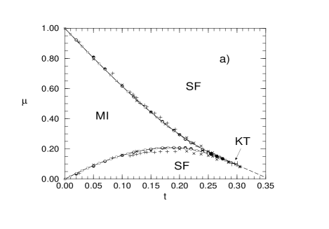
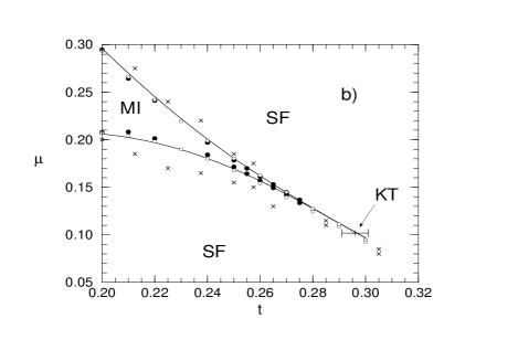
FIG. 9.: The phase diagram with on-site interactions only (MI:Mott-insulator with density one, SF:superfluid phase). The solid lines show a Padé analysis of 12th order strong coupling expansions [30], two different sets of Quantum Monte Carlo data are “+”[31] and “x” [32]. The filled circles show older DMRG results[33], the empty boxes are the new DMRG data. The dashed lines indicate the area with integer density. The error bars in the $\mu$ direction are smaller than the circles, the error bar in the $t$ direction is the error of $t_{c}$ for the Kosterlitz-Thouless (KT) transition.

FIG. 10.: Same as 10, with the tip of the Mott-insulator on an expanded scale.

Using the methods described above we determine the phase diagram in the presence of on-site interactions only. Fig. 10 shows the Mott-insulator with density $\rho=1$, surrounded by the superfluid phase. In Fig. 10 the tip of the insulator is shown on an expanded scale. The very pointed tip of the insulating region reflects the closing of the energy gap given by Eq. (6). Fig. 10 also shows results for the commensurate-incommensurate phase transition from twelfth order perturbation theory. The excellent agreement with DMRG confirms the high accuracy achieved.

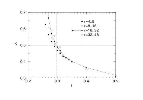
FIG. 11.: $K$ vs $t$ at the Kosterlitz-Thouless transition from the density one Mott-insulator to the superfluid phase. The critical point is determined by finding the $t$ at which $K=1/2$. The biggest system sizes are $L=256$ sites except for $t=0.29,0.3,0.31$, where they are $L=1024$.

TABLE I.: The location of the critical point $t_{c}$ depending on the interval of $r$ used for the fits to $\Gamma(r)=\langle b^{\dagger}_{r}b_{0}\rangle$.

$r$	$t_{c}$
$4\leq r\leq 8$	$0.2874\pm 0.0001$
$8\leq r\leq 16$	$0.2938\pm 0.0001$
$16\leq r\leq 32$	$0.2968\pm 0.0003$
$32\leq r\leq 48$	$0.3062\pm 0.0003$
$48\leq r\leq 64$	$0.3107\pm 0.01\phantom{00}$

To find the critical point of the Kosterlitz-Thouless transition at the tip of the Mott-insulator, we determine the $t$ at which $K=1/2$. As described in Section V B, the $K$ are determined by fitting power-law behavior to the decay of the hopping correlation function $\Gamma(r)=\langle b^{\dagger}_{r}b_{0}\rangle$. Due to finite-size effects, the result can depend on the interval of $r$ that is used for this fit. While we found $16\leq r\leq 32$ to be reasonable in general, there are logarithmic finite-size effects at the Kosterlitz-Thouless transition that require a more detailed inspection. Fig. 11 shows $K$’s that were determined with different fitting intervals plotted versus $t$.

For the $t=0.29$, $t=0.3$ and $t=0.31$ systems with $L=512$ and $L=1024$ sites were calculated to keep finite-size effects small. Table I shows the $t_{c}$ found with different fitting intervals. Due to the finite-size effects the $t_{c}$ go to higher $t$ as the fitting interval is shifted to bigger $r$. While using a fitting interval of $16\leq r\leq 32$ is a good compromise between avoiding finite-size effects by using small $r$, and finding an asymptotic value for the decay by using big $r$, the error determined by this fit alone underestimates the true error. With an error estimated from the effect of the choice of the fitting interval, we find $t_{c}=0.297\pm 0.01$.

Determination of the Kosterlitz-Thouless transition was attempted in several previous studies. For a truncated model with a maximum of two particles per site the critical point was found at $t_{c}^{BA}=1/(2\sqrt{3})\approx 0.289$ with the Bethe-Ansatz[34]. In a combination of exact-diagonalization for system with up to $L=12$ sites and renormalization group Kashurnikov and Svistunov found $t_{c}=0.304\pm 0.002$[35], and together with Kravasin found $t_{c}=0.300\pm 0.005$[32] in a quantum Monte Carlo study. An exact diagonalization approach reported the critical point to be at $t_{c}=0.275\pm 0.005$[36], and a study using 12th order strong coupling expansions[30] located it at $t_{c}=0.26\pm 0.01$.

There were two previous studies using DMRG to locate the Kosterlitz-Thouless transition in the Bose-Hubbard model. In the first study[37] a particle cut-off of $n=4$ per site was used, and the critical point was determined by using a phase twist $\phi=\pi$ and periodic boundaries to calculate the superfluid stiffness. The critical point was found at $t_{c}=0.298$. In another DMRG study[33], the critical point was found at $t_{c}=0.277\pm 0.01$ by determining the $t$ at which $K=1/2$, similar to the procedure used in the present work. In both of these DMRG studies the numerical accuracy was limited due to the use of the infinite size version of the DMRG algorithm, periodic boundary conditions and a small number of states in the DMRG basis. The biggest system sizes were smaller than $L=80$.

The range of these results demonstrates the difficulty involved in determining the critical point of the Kosterlitz-Thouless transition, which is mostly due to logarithmic finite-size effects close to the critical point. The large system sizes used in this paper should compensate for this within the given error bars, and yield a reliable result.

The phase diagram shown in Fig. 10 has a very interesting feature. Imagine moving on a line of constant chemical potential $\mu$, for example $\mu=0.15$, and starting at small $t$, moving toward bigger $t$. The particle density along this line is illustrated in Fig. 12. For small $t$ the system is in the Mott-insulator phase. At $t\approx 0.1$ there is a phase transition to the superfluid phase, with densities $\rho<1$. The density decreases up to a minimum, then it start increasing again. At $t\approx 0.26$ the density goes up to $\rho=1$ again, and there is another phase transition, this time reentering the Mott-insulating phase from the superfluid phase. Increasing $t$ further leads to another phase transition from the Mott-insulator to the superfluid phase, this time with $\rho>1$, and the density increasing further with increasing $t$.

FIG. 12.: Illustration of the phase transitions between the Mott-insulator (MI) and the superfluid phase (SF) on a line of constant chemical potential $\mu=0.15$.

FIG. 13.: The Mean-Field phase diagram[38] in dimensionless units, showing lines of constant density.

To gain more insight into this, we compare to results from a mean field approach[38]. Fig. 13 shows the phase diagram with the Mott-insulator at density $\rho=1$, surrounded by the superfluid phase. In the superfluid phase, the lines of constant density slope downward as $t$ is increased. This is not only found in one dimension, but in all dimensions. The limit of $t\rightarrow\infty$ corresponds to keeping $t$ constant and setting the interactions to zero. If the interactions are zero the system goes from a superfluid phase to a Bose-Einstein condensate, in which every particle has an energy of $-2t$. If the chemical potential is smaller than $-2t$, the system is empty, because it costs energy to put a particle in, and for chemical potentials bigger than $-2t$ the number of particles goes to infinity, because every additional particle reduces the total energy of the system. Going back to the picture of constant interactions and changing $t$, this means that the density of the system always goes to infinity as $t$ is increased.

In dimensions two and higher the superfluid-insulator transition on the line of constant density is a second order transition, and the tip of the insulating region is round. Fig. 14 shows the density on a line of constant chemical potential $\mu=0.3$. At the phase transition from the Mott-insulator to the superfluid phase the density first drops as $t$ is increased, and then increases again.

In one dimension the tip of the insulating region is very long and narrow due to the Kosterlitz-Thouless transition, and it is possible to reenter into the insulator at $\rho=1$.

FIG. 14.: The density on a line of constant chemical potential $\mu=0.3$ in the Mean-Field phase diagram (Fig. 13).

VII Nearest-neighbor interaction

Longer ranger interactions have been found to be important in experiments[7, 8, 9]. We now include nearest-neighbor interactions by setting $V=0.4$. Due to the nearest-neighbor interactions a new insulator phase appears at half integer densities. It is a charge density wave phase (CDW) with a wavelength of two sites, and like the Mott-insulator at integer density it has an excitation gap and is incompressible. The crystalline order is characterized by a non-zero structure factor

$$S_{\pi}=\frac{1}{N^{2}}\sum_{ij}(-1)^{\mid i-j\mid}\langle n_{i}n_{j}\rangle\;.$$ (12)

In Fig. 6 the local density oscillations in the charge density wave phase are shown. A small boundary effect can be seen, but the main feature are long-range density oscillations throughout the system that do not decay. An order parameter $\langle n_{i}-\rho\rangle$ can be defined to describe this charge density wave, even in one dimension.

In one dimension the superfluid phase is signalled by a diverging correlation length

$$\xi^{2}=\sum_{r}r^{2}\langle b^{\dagger}_{r}b_{0}\rangle/\sum_{r}\langle b^{\dagger}_{r}b_{0}\rangle\;,$$ (13)

and a non-zero superfluid stiffness

$$\rho_{s}=\lim_{\phi\rightarrow 0}L\frac{\partial^{2}E_{0}(\phi,L)}{\partial\phi^{2}}\;,$$ (14)

which is proportional to the Drude weight $D\sim\rho_{s}$. In two and higher dimensions there is also an order parameter $\langle b^{\dagger}_{i}\rangle\neq 0$. In one dimension the whole superfluid phase is critical, and there is no order parameter.

At the transition from the charge density wave phase to the superfluid phase both types of order are involved: the crystalline order in the charge density wave phase and the superfluid order in the superfluid phase. In addition to a direct phase transition from the charge density wave to the superfluid at which the crystalline order vanishes at the same point where the superfluid order appears, there is the possibility of an intermediate phase. Tab. II shows the possible phases close to density $\rho=1/2$ in a bosonic system with on-site and nearest-neighbor interaction in two or higher dimensions. In addition to the charge density wave and the superfluid phase, supersolids that have both forms of order were found in two dimensional models[10, 11]. Baltin and Wagenblast[14] found a region that has neither superfluid stiffness nor charge density wave in a one dimensional bosonic model in the high density. The possible existence of such a phase was also recently predicted for a two dimensional bosonic model in the high density limit by Das and Doniach[15], who call it a Bose-metal.

TABLE II.: Possible phases and their order parameters close to density $\rho=1/2$.

$S_{\pi}$	$\rho_{s}$	phase
$\neq 0$	$=0$	charge density wave
$=0$	$\neq 0$	superfluid
$\neq 0$	$\neq 0$	supersolid
$=0$	$=0$	Bose-metal

In Appendix C strong coupling expansions are used to illustrate the difference between the commensurate-incommensurate phase transition at $\rho=1/2$ in one and two dimensions. Strong coupling expansions can be used to study the insulator, but not the superfluid. To study the low-energy behavior of the superfluid phase the Luttinger liquid can be used. In addition to the basic Luttinger liquid Hamiltonian (Eq. (7)), the lattice and the interactions introduce scattering terms (Eq. (10)). These only contribute at $\rho=1/2$, where they can drive the system into a different phase, but not at nearby densities. At incommensurate densities close to $\rho=1/2$, the wavefunction is incommensurate with the lattice and hence cannot be pinned to the lattice to form an insulator. Of course this would be changed if there were impurities or disorder, but a pure system in one dimension is in the Luttinger liquid phase unless it is at a density commensurate with the lattice and the interactions.

At density $\rho=1/2$ DMRG can be used to determine if there is an intermediate phase or a direct phase transition from the charge density wave phase to the superfluid phase. To do this, we investigate the relationship between the superfluid and crystalline order at the phase transition. The onset of superfluidity is signaled by a diverging correlation length $\xi$ (Eq. (13)), charge density order is meassured by $S_{\pi}>0$ (Eq. (12)).

The model is in the universality class of the xy-model at the phase transition on the line of constant density at $\rho=1/2$. Due to the Kosterlitz-Thouless transition expected on this line, it is difficult to determine exactly when the structure factor or the inverse correlation length go to zero. But it is possible to study the dependence of the structure factor on the correlation length. Fig. 15 shows that for small values the structure factor depends on the correlation length by a power-law:

$$\xi(S_{\pi})^{-1}-\xi(S_{\pi}=0)^{-1}\sim(S_{\pi})^{\alpha}\;.$$ (15)

To keep the effect of the boundaries small for the calculation of both the structure factor $S_{\pi}$ and the correlation length $\xi$, only sites that were at least a quarter of the system size away from the boundaries were taken into account.

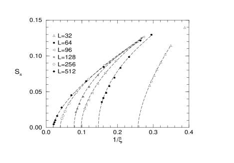
FIG. 15.: Structure factor $S_{\pi}$ versus the inverse correlation length $\xi$ for different system sizes. The dashed lines show power-law fits.

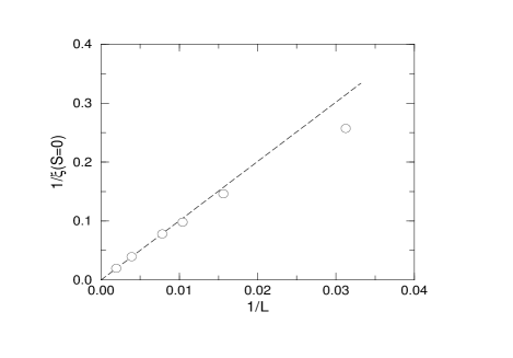
FIG. 16.: The inverse correlation length $1/\xi$ at $S_{\pi}=0$ obtained from Fig. 15 versus the inverse system size. The dashed line shows a linear fit to the three biggest system sizes.

In Fig. 16 the extrapolated inverse correlation length $1/\xi(S_{\pi}=0)$ at zero structure factor is plotted against the inverse system size. The linear fit to the three biggest system sizes shows that $1/\xi(S_{\pi}=0)$ goes to zero for infinite systems. From this and the power-law behavior in Fig. 15 we conclude that there is a power-law dependence of the structure factor on the correlation length, and that in infinite systems the correlation length diverges at the same point at which the structure factor goes to zero. This means that there is a direct phase transition from the charge density wave phase to the superfluid phase, and no supersolid or normal phase in between.

FIG. 17.: Illustration of the lines of constant $K$ in the phase diagram. The dotted lines indicate $K$ that are slightly smaller or bigger than $K=1$.

The phase boundaries of the charge density wave phase can be found in the same way as those of the Mott-insulator, and we use the methods used for the on-site only interaction case to calculate the phase diagram. Fig. 18 shows the phase diagram in the region of the $\rho=1/2$ charge density wave phase and the $\rho=1$ Mott-insulator. Like the shape of the Mott-insulator with on-site interaction only, the shapes of the insulating regions reflect the Kosterlitz-Thouless transitions at the tips. The tips are also bending down, allowing re-entrance phase transitions from the superfluid to the insulating phases. We find the Kosterlitz-Thouless transitions at $t_{c}^{MI}=0.404\pm 0.02$ for the Mott-insulator, and at $t_{c}^{CDW}=0.125\pm 0.003$ for the charge density wave phase. The critical point at the tip of the charge density wave phase had been found in a quantum Monte Carlo study at $t\approx 0.1$. The accuracy of $t_{c}^{MI}$ is relatively low because $K$ only changes very slowly if $t$ is changed close to this transition. This had already been observed in an earlier DMRG study[33], where the critical points were found at $t_{c}^{CDW}=0.118\pm 0.004$ and $t_{c}^{MI}\approx 0.325\pm 0.05$. That study used the infinite size version of the DMRG, and the biggest systems were $L=76$ sites long. Since there are logarithmic finite-size effects at the Kosterlitz-Thouless transitions, the values determined in the present work, where systems with up to $L=512$ sites are used, are much more accurate.

At the phase boundaries of the charge density wave phase the Luttinger Liquid parameter is $K=4$ except for the Kosterlitz-Thouless transition at the tip, where it is $K=2$. The charge density wave phase is surrounded by a region where $K>1$. The effective interactions in the Luttinger-Liquid are attractive for $K<1$ and repulsive for $K>1$. Kane and Fisher showed that in the repulsive region a single impurity turns the system into an insulator[17, 27]. An even larger region of the Luttinger liquid is driven into a glass phase if $K>2/3$ for any finite quenched disorder[18, 1].

In the phase diagram these regions ($K>1$ and $K>2/3$) are determined by doing calculations for different densities and $t$. For example, to determine the $t$ for which $K(t)=1$ at a given density $\rho$, we do calculations for different $t$ until we find a pair of $t_{1}$ and $t_{2}$ that are close to each other, and $K(t_{1})>1>K(t_{2})$. We then determine $t(K=1)$ by linear interpolation. To find the boundaries of the repulsive Luttinger Liquid region, we calculate $t(K=1)$ for various densities.

The lines with $K=1$ and $K=2/3$ are shown in Fig. 18. The repulsive Luttinger Liquid ($K>1$) region completely surrounds the charge density wave phase. Instead of going to $t=0$ as the Mott-insulator is approached, the $K=1$ line ends in the side of the Mott-insulating region, where $K=1$ for all of the commensurate-incommensurate phase boundary. Fig. 17 illustrates how the two lines with $K=1$ meet at the phase boundary of the Mott-insulator. Although we could not obtain more detailed results for densities closer to $\rho=1$, we argue that the lines with $K>1$ bend towards $t=0$ as the density gets closer to one, while those with $1/2<K<1$ bend towards the tip of the Mott-insulator.

Lines of constant $K$ with $1/2<K<1$ are discontinuous at $\rho=1$, where the system is an insulator for $K>1/2$, with the tipped shape reflecting the Kosterlitz-Thouless behavior. Lines with $K\leq 1/2$ are round at $\rho=1$, and do not reflect the Kosterlitz-Thouless behavior. Analogous to $\rho=1$, we also observe that the lines of constant $K$ are round for $K\leq 2$ and $\rho=1/2$, where the charge density wave phase ends in a Kosterlitz-Thouless transition at $K=2$.

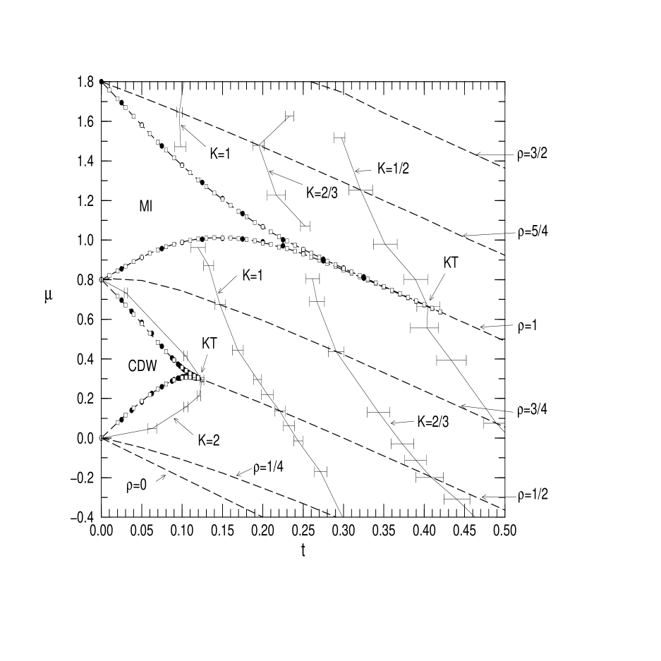
FIG. 18.: The phase diagram of the Bose-Hubbard model with nearest-neighbor interaction $V=0.4$. The Mott-insulator (MI) at density $\rho=1$ and the charge density wave phase (CDW) at density $\rho=1/2$ are surrounded by the superfluid phase. The long-dashed lines show the lines of constant density. The solid lines are lines of constant $K$. The $K=2$ line crosses the density $\rho=1/2$ line at the Kosterlitz-Thouless (KT) transition at the tip of the charge density wave phase. In the region left of the $K=1$ line, where $K>1$, the superfluid phase is turned into an insulator by a single impurity[17]. In the presence of disorder the region left of $K=2/3$ line is turned into a Bose-glass phase[18, 1]. The Kosterlitz-Thouless (KT) transition at the tip of the Mott-insulator is at the point where the $K=1/2$ line line intersects the $\rho=1$ line.

VIII ac-conductivity

The repulsive region of the Luttinger liquid is turned into an insulator by a single impurity[17]. This raises the question if there is a qualitative difference between the conductivity in the repulsive region and the attractive region of the Luttinger liquid in the pure system. The regular part of the conductivity is given by:

$$\sigma_{1}^{reg}(\omega) = \frac{1}{L}\sum_{m\neq 0}\frac{{|\langle m\mid j_{q=0}\mid 0\rangle|}^{2}}{E_{m}-E_{0}}\delta{(\omega-(E_{m}-E_{0}))}$$ (16)

$$= -\frac{1}{\omega\,\pi\,L}\text{Im}\lim_{\eta\rightarrow 0^{+}}$$ (18)

$$\langle 0\mid j^{\dagger}_{q=0}\frac{1}{\omega+E_{0}-H+i\eta}j_{q=0}\mid 0\rangle\;,$$

and the current operator is

$$j_{q}=it\sum_{n}e^{-iqn}(b^{\dagger}_{n+1}b_{n}-h.c.)\;.$$ (19)

Recent developments with DMRG make the calculation of dynamical correlation functions like the ac-conductivity possible[39]. The conductivity at a frequency $z=\omega+i\eta$ can be calculated as the direct product of the current operator applied to the groundstate

$$\mid j_{q=0}\rangle=j_{q=0}\mid 0\rangle\;,$$ (20)

and a correction vector

$$\mid x(z)\rangle=\frac{1}{\omega+E_{0}-H+i\eta}\mid j_{q=0}\rangle\;.$$ (21)

By using these two states and the groundstate $|0\rangle$ as DMRG target states, the conductivity $\sigma_{1}^{reg}(z)$ can be calculated very precisely. To calculate the conductivity over an interval of width $\eta$ ranging from $\omega_{1}$ to $\omega_{2}$, we use correction vectors $\mid x(\omega_{1}+i\eta)\rangle$ and $\mid x(\omega_{2}+i\eta)\rangle$ as target states. At the end of the DMRG calculation, when the DMRG basis is optimized to represent these states, we calculate the conductivity from $\omega_{1}$ to $\omega_{2}$. Repeating this procedure for neighboring intervals, we piece together the conductivity for a whole range of frequencies.

The finite broadening $\eta$ in the correction vectors is only used to obtain appropriate DMRG target states. To calculate the spectrum within the DMRG basis, we use a Lanczos method that yields approximate eigenstates of the Hamiltonian. The broadening used in our plots is then applied to the discrete peaks found with the Lanczos method, and is only used for better visualization.

DMRG calculations work best with open boundary conditions. How the current operator is applied in a system with open boundary conditions is discussed in Appendix D.

FIG. 19.: The conductivity $\sigma_{1}^{reg}(\omega)$ in the Mott-insulator at density $\rho=1$, $t=0.05$, $U=1$, $V=0.4$, system size $L=256$, $m=128$ states, two correction vectors as target states with $\eta=0.05$, and broadening $\eta_{g}=0.01$ for the plot. The inset shows the same data on an expanded scale.

The conductivity in the Mott-insulator phase is shown in Fig. 19. There is an energy gap of $\Delta\omega=0.54$, with a big peak after that and only small excitations at higher energies. Since it is an insulator phase, we expect to find no Drude weight. With the kinetic energy defined as

$$\langle T\rangle=t\sum_{n}\langle b^{\dagger}_{n+1}b_{n}+h.c.\rangle\;,$$ (22)

the Drude weight is given by

$$D=-\frac{1}{L}\langle T\rangle-2\int d\omega\;\sigma_{1}^{reg}(\omega)\;.$$ (23)

Note that the Drude weight is proportional to the superfluid stiffness $\rho_{s}$ given in Eq. (14).

Since the kinetic energy $\langle T\rangle$ can be calculated directly with DMRG, and we expect $D=0$, this is an opportunity to verify the consistency of the calculation. In Tab. III the Drude weight is shown for various system sizes. A small finite-size effect can be seen in the data. From the differences in the individual values we estimate the error of the Drude weight $\Delta D=0.02t$, or $2\%$ of $-\langle T\rangle/L$.

TABLE III.: The Drude weight $D$ for different system sizes in the Mott-insulator with density $\rho=1$, $t=0.05$, $U=1$,$V=0.4$. $\langle T\rangle$ is the kinetic energy, $\int\sigma_{1}^{reg}(\omega)d\omega$ the integral over the ac-conductivity. Also shown is the number of states $m$, the broadening $\eta$ of the correction vectors, and the truncation error $\Delta$.

$L$	$D/t$	$\langle T\rangle/(tL)$	$2/t\int\sigma_{1}^{reg}(\omega)d\omega$	$\eta$	$m$	$\Delta$
32	0.0084	0.6392	0.6307	0.05	128	$10^{-7}$
64	-0.0040	0.6392	0.6432	0.05	128	$10^{-7}$
128	-0.0075	0.6392	0.6467	0.05	128	$10^{-7}$
256	-0.0036	0.6392	0.6428	0.05	128	$10^{-7}$

FIG. 20.: The precursor peaks in the conductivity $\sigma_{1}^{reg}(\omega)$ in the repulsive region of the superfluid phase at density $\rho=3/4$, $t=0.05$, $U=1$, $V=0.4$, system size $L=128$ and $m=128$ states. Broadening $\eta=0.02$ for correction vectors, and $\eta_{g}=0.005$ for the plot.

In the superfluid phase we find precursor peaks at small frequencies in the conductivity. They are due to the finite width[39] of the wavevector $q$, which is $\Delta q=4\sqrt{3}/L$. Fig. 20 shows these precursor peaks in the repulsive Luttinger liquid for different system sizes. As the system size is increased the precursor peaks move towards $\omega=0$. For the calculation of the Drude weight these peaks should not contribute, and we use low-energy cut-offs to ignore them.

FIG. 21.: The conductivity $\sigma_{1}^{reg}(\omega)$ in the repulsive region of the superfluid phase at density $\rho=3/4$, $t=0.05$, $U=1$, $V=0.4$. Data shown is for different system sizes with ($L=64$,$m=256$,$\eta=0.05$), ($L=128$,$m=256$,$\eta=0.05$) and ($L=256$,$m=512$,$\eta=0.2$). Broadening $\eta_{g}=0.05$ for the plot, and the low-frequency cut-offs given in Tab.IV.

FIG. 22.: The conductivity $\sigma_{1}^{reg}(\omega)$ in the attractive region of the superfluid phase at density $\rho=3/4$, $t=0.5$, $U=1$, $V=0.4$. System size $L=32$ and $L=64$ with $m=128$ states, and $L=128$ with $m=256$ states. Broadening $\eta=0.2$ for the correction vectors, $\eta_{g}=0.2$ for the plot, and the low-frequency cut-offs given in Tab. V.

TABLE IV.: The Drude weight $D$ for different system sizes in the repulsive region of the superfluid phase at density $\rho=3/4$, $t=0.05$, $U=1$,$V=0.4$. Same notation as in Tab.III.

$L$	$D/t$	$\langle T\rangle/(tL)$	$2/t\int\sigma_{1}^{reg}(\omega)d\omega$	$\eta$	$m$	$\Delta$	$\omega_{c}$
16	0.776	0.874	0.099	0.2	128	$5\times 10^{-7}$	0.2
32	0.791	0.885	0.094	0.2	128	$7\times 10^{-7}$	0.1
64	0.799	0.890	0.091	0.2	128	$5\times 10^{-6}$	0.08
64	0.798	0.890	0.092	0.05	256	$1\times 10^{-6}$	0.08
128	0.799	0.892	0.093	0.2	128	$7\times 10^{-6}$	0.02
128	0.801	0.892	0.091	0.1	256	$6\times 10^{-7}$	0.02
128	0.793	0.892	0.099	0.05	128	$1\times 10^{-5}$	0.02
128	0.797	0.892	0.095	0.05	256	$1\times 10^{-6}$	0.02
256	0.800	0.893	0.093	0.2	512	$5\times 10^{-7}$	0.02

Fig. 21 and Fig. 22 show the conductivity in the superfluid phase in the repulsive and attractive Luttinger liquid regions. In the Luttinger liquid the conductivity was predicted to increase with a power-law for small frequencies, and decay exponentially for big frequencies[24, 25]. The conductivity in the attractive region shown in Fig. 22 is in good qualitative agreement with this. In the repulsive case (Fig. 21) there are too few peaks to clearly identify this behavior. Bigger systems would have to be studied to determine if the overall shape is qualitatively different from the attractive region.

The Drude weight in the repulsive and attractive regime of the superfluid phase is shown in Tab. IV and Tab. V. For some system sizes data with different numbers of states $m$ and broadening $\eta$ is shown. The numerical accuracy depends on these parameters, with bigger $m$ and smaller $\eta$ for higher accuracy. The data in Tab. IV and Tab. V shows that the impact of $m$ and $\eta$ on the Drude weight is small. In both the attractive and repulsive case we find big non-zero values that are close to the kinetic energy per site in the systems. The differences in the Drude weight in different system sizes, with the exception of the smallest systems, are rather due to numerical errors that grow with the system size, than due to finite-size effects.

TABLE V.: The Drude weight $D$ for different system sizes in the attractive region of the superfluid phase at density $\rho=3/4$, $t=0.5$, $U=1$,$V=0.4$. Same notation as in Tab.III.

$L$	$D/t$	$\langle T\rangle/(tL)$	$2/t\int\sigma_{1}^{reg}(\omega)d\omega$	$\eta$	$m$	$\Delta$	$\omega_{c}$
32	1.438	1.444	0.006	0.2	128	$10^{-4}$	0.6
64	1.421	1.427	0.006	0.2	128	$10^{-4}$	0.4
128	1.412	1.417	0.005	0.2	128	$10^{-4}$	0.3
128	1.411	1.417	0.006	0.2	256	$10^{-5}$	0.3

IX Conclusions

In summary, we have studied the phase diagram of the one-dimensional Bose-Hubbard model with on-site only interactions and with additional nearest-neighbor interaction. The density matrix renormalization group (DMRG) was used to calculate chemical potentials for given densities and model parameters, and by doing this for sets of parameters the phase boundaries of the Mott-insulators and the charge density wave phase were determined.

The low-energy behavior of the superfluid phase of one-dimensional bosonic systems is that of a Luttinger liquid. We determined the Luttinger liquid parameter $K$ from the decay of the hopping correlation functions. Since the value of $K$ is known for insulator-superfluid transitions, we could use it to locate the Kosterlitz-Thouless transitions at the tips of the Mott-insulators and the charge density wave phase in the $\mu$-$t$ phase diagram.

In the charge density wave phase we found that close to the phase transition the structure factor depends on a power-law of the superfluid correlation length. From this we conclude that there is a direct phase transition from the charge density wave phase to the supersolid, and no intermediate phase like a supersolid or normal phase.

The charge density wave phase is surrounded by a region of the superfluid phase where $K>1$, which corresponds to a Luttinger liquid with repulsive effective interactions. Kane and Fisher have shown that this region will be turned into an insulator by a single impurity. We determined the boundary of the repulsive region by finding the line where $K=1$ in the phase diagram. We found that this boundary does not go to $t=0$ as the Mott-insulator is approached, but ends in the side of the Mott-insulating region, where the Luttinger liquid parameter also is $K=1$.

We calculated the ac-conductivity in the Mott-insulator and the superfluid phase. In the Mott-insulator and the attractive region of the superfluid phase the ac-conductivity has the expected shape. In the repulsive region of the Luttinger liquid we found a different shape, but could not determine if this is due to the finite system sizes. The Drude weight or superfluid stiffness was found to be big in both the attractive and the repulsive region.

X Acknowledgments

The authors would like to thank H. Carruzzo, J. K. Freericks, T. Giamarchi, L. I. Glazman, V. A. Kashurnikov, A. J. Millis and R. T. Scalettar for valuable discussions. This work was supported by the National Science Foundation under grant DMR98-70930 and the DAAD “Doktorandenstipendium im Rahmen des gemeinsamen Hochschulsonderprogramms III von Bund und Ländern”.

A Truncation of the model

FIG. 23.: The $\Gamma(r)=\langle b^{\dagger}_{r}b_{0}\rangle$ correlation function for various truncations of the maximum number of particles per site $n_{max}$ in the Mott-insulator at density $\rho=1$ in a $L=128$ system with $t=0.1$ and $V=0.4$. For $n_{max}\geq 3$ the different correlation functions become indistinguishable.

The number of possible states per site in the Bose-Hubbard model is infinite since there can be any number of particles on a site. For practical DMRG calculations we truncate the model by only allowing a maximum number of particles $n_{max}$ on each site. Pai et al. [37] chose $n_{max}=4$ in a DMRG study, while Kashurnikov and Svistunov[35] used $n_{max}=3$ in a Quantum Monte Carlo study. To verify the effect of this truncation on the correlation function $\Gamma(r)=\langle b^{\dagger}_{r}b_{0}\rangle$, we calculate systems with different $n_{max}$. Fig. 23 shows $\Gamma(r)$ in the Mott-insulator. Due to the small particle-hole excitations, the correlation functions are almost identical for $n_{max}\geq 3$. In the superfluid phase there are more particle-hole excitations which are affected by the truncation. Fig. 24 shows that the correlation functions are independent of $n_{max}$ for $n_{max}\geq 4$. By choosing $n_{max}=5$ for all calculations the effect of the truncation should be small enough not to affect the results presented in this work.

FIG. 24.: The $\Gamma(r)=\langle b^{\dagger}_{r}b_{0}\rangle$ correlation function for various $n_{max}$ in the superfluid phase in a $L=128$ system with $\rho=1$, $t=0.5$ and $V=0.4$.

B Truncation of the DMRG basis

FIG. 25.: The $\Gamma(r)=\langle b^{\dagger}_{r}b_{0}\rangle$ correlation function for various truncation errors $\Delta$ in the $\rho=1$ Mott-insulator phase. System size $L=128$, $t=0.1$ and $V=0.4$.

In every DMRG step the basis is truncated, and only the eigenstates of the density matrix with the biggest eigenvalues are kept. The density matrix weight of the discarded states $\Delta$ is a measure of the error caused by these truncations. To verify to which extent the truncation errors affect the results, we calculate the correlation function $\Gamma(r)=\langle b^{\dagger}_{r}b_{0}\rangle$ with different numbers of states kept in the DMRG basis. Fig. 25 shows $\Gamma(r)$ with different truncation errors in the Mott-insulator. Even for very small numbers of states the discarded weight is very small, and the dependence on the weight of the discarded states is weak. Note that the discrepancies are mostly apparent due to the logarithmic scale.

FIG. 26.: The $\Gamma(r)=\langle b^{\dagger}_{r}b_{0}\rangle$ correlation function in the superfluid phase at $\rho=1$ for various truncation errors. System size $L=128$, $t=0.5$ and $V=0.4$.

FIG. 27.: $\mu^{+}$ versus the discarded weight $\Delta$ in the Mott-insulator at $\rho=1$. The scale for $\Delta$ is logarithmic on the left plot and linear on the right plot. The system size is $L=128$, $t=0.1$ and $V=0.4$.

The correlation function in the superfluid phase is shown in Fig. 26. We find that the discarded weight with the same number of states is bigger than it is in the insulator. At small distances $r$ the correlation functions are very similar for all numbers of states, with increasing differences as $r$ is increased. If the discarded weights $\Delta$ are smaller than $8\times 10^{-8}$, the correlation functions coincide even at the boundaries of the system. By requiring the discarded weight to be smaller than $\Delta\leq 10^{-9}$ for the calculation of the correlation functions, accuracy should be high enough in all cases.

The chemical potentials are calculated from the energies it takes to add a particle or hole. Figures 27 and 28 show chemical potentials calculated with different numbers of states kept versus the discarded weight $\Delta$. The error bars correspond to the changes in the energies during a DMRG sweep. Differences in the chemical potentials are small for $\Delta<10^{-5}$. We require the discarded weight to be smaller than $\Delta<5\times 10^{-6}$ for the calculations of the chemical potentials, and to improve the results further, we extrapolate linearly from the two values with the lowest $\Delta$.

FIG. 28.: $\mu^{+}$ and $\mu^{-}$ versus discarded weight $\Delta$ in the superfluid phase. The scale for $\Delta$ is logarithmic on the left plot and linear on the right plot. The density is $\rho=1$, system size $L=128$ and $t=0.5$ and $V=0.4$.

C Strong coupling expansion at the commensurate-incommensurate transition

The fundamental difference between the commensurate-incommensurate phase transition at $\rho=1/2$ in one and two dimensions can be illustrated with the help of a strong coupling expansion. In the strong coupling limit the kinetic energy is zero. The zero order states are the groundstates of the Hamiltonian only including the particle-particle repulsion:

$$H = U\sum_{i}n_{i}(n_{i}-1)/2+V\sum_{i}n_{i}n_{i+1}\;.$$ (C1)

The series expansion is made in terms of the kinetic energy term:

$$H^{\prime}=-t\sum_{\langle i,j\rangle}(b^{\dagger}_{i}b^{\phantom{\dagger}}_{j}+h.c.)\;.$$ (C2)

Strong coupling expansions of this type have been successfully used to study the phase diagram with on-site only interaction[30, 40, 41]. To determine the phase boundaries of the Mott-insulator at $\rho=1$, first the groundstate of Eq. (C1) has to be found. In this state there is simply one boson sitting on every site. Higher terms of the perturbation series introduce local particle-hole excitations. The chemical potentials on the boundaries can be determined from the energy it costs to add a particle (Eq. (4)) or a hole (Eq. (5)). But in these cases, the zeroth order ground state is degenerate, since the additional particle or hole can sit on any site. This degeneracy is lifted in first order perturbation theory. In first order the problem is reduced to the additional single particle moving on a uniform background of completely localized particles. Since the extra particle gains energy by hopping from site to site, it becomes completely delocalized. Although this behavior can be modified in higher order of the perturbation series, and there are limitations due to the radius of convergence, it is interesting to note the difference between the perturbation series in the insulator and with an additional particle or hole. At integer density the series starts out with a completely localized state, while it starts with a completely delocalized state if there is an additional particle or hole. This is in good agreement with the fact that there is a Mott-insulator for small $t$ at integer density, and a direct phase transition to a superfluid (delocalized) phase if the density is changed.

A similar strong coupling expansion can also be used at the charge density wave phase at $\rho=1/2$. The charge density wave phase at $t=0$ is a state with alternating particle numbers, in one as well as two dimensions (Fig.29 and Fig.30). Higher order terms in the perturbation series introduce local particle hopping without destroying the charge density wave order.

FIG. 29.: The CDW in 2-d at $t=0$.

FIG. 30.: The CDW in 1-d at $t=0$.

At the commensurate-incommensurate transition, an additional particle (or hole) enters the system. For $V<U/2$ the energy is smallest if the additional particle goes to one of the empty sites. Fig. 31 shows how the additional particle fits into the two-dimensional charge density wave. In higher orders of perturbation theory the additional particle, as well as particle-hole excitations, hop on the charge-density background without destroying it. From this we cannot infer if the true (non-perturbation theory) groundstate is superfluid or not, and if the charge density wave order is destroyed by the particle hopping. Nevertheless, it is interesting to note that for this case supersolids have been found[10, 11] in two dimensions. Close to the charge density wave phase at $\rho=1/2$, the charge density order survives at small doping.

FIG. 31.: CDW with additional particle in 2-d at $t=0$.

FIG. 32.: Additional particle in 1-d at $t=0$. The thick lines are the domain walls. $\phi_{0}$ is the phase of the charge density wave.

In contrast to this, the one-dimensional case looks quite different. The additional particle also goes to an unoccupied site. If the charge density wave remains unchanged, the additional energy is $\Delta E=2V$. With the structure factor $S_{\pi}$, the charge density wave is given by an order parameter $\langle n_{l}\rangle=\rho+S_{\pi}\exp{(i\pi l+i\phi_{0})}$. An additional particle or hole can also be added by shifting the phase $\phi_{0}$ by $\pi$ over a region with an odd number of sites. Fig.32 shows an example of such a state. In the center there is a domain with a $\pi$ phase shift, and the number of particles compared to the charge density wave (Fig.29) is increased by one. And the additional energy is also $\Delta E=2V$. To lift the degeneracy between all these states in first order perturbation theory, it can be seen that a particle hopping next to the domain boundary is equivalent to the domain wall moving. Since energy is gained by this, the domain walls are completely delocalized in first order perturbation theory. Unlike the two dimensional case, where the charge density wave order survives in all orders, in one dimension it is destroyed in first order. While a perturbation series does not necessarily converge, this striking feature illustrates the fundamental difference between the one and two dimensional case.

D Current operator with open boundaries

FIG. 33.: The conductivity $\sigma_{1}^{reg}(\omega)$ in the insulator with periodic and open boundary conditions. The density is $\rho=1$, $t=0.05$, $U=1$ and $V=0.4$, system size $L=32$, and $m=128$ states. Broadening $\eta=0.2$ for the correction vectors, and $\eta_{g}=0.01$ for the plot. The inset shows the data on an expanded scale.

DMRG calculations work best with open boundary conditions. To calculate the conductivity with DMRG, the current operator has to be implemented. The current operator as it is given in Eq. (19) can be used directly with periodic boundary conditions, but to apply the current operator with open boundary conditions we modify it with a filter function:

$$j_{q=0}=\sum_{n=-\infty}^{\infty}P(x_{n}/M)(b^{\dagger}_{n+1}b_{n}-h.c.)\;.$$ (D1)

The filter function $P(x_{n}/M)$ used here is a Parzen filter, $x_{n}$ is the distance of site $n$ from the middle of the system, and $M=L/2$ is half the system size. The Parzen filter looks very similar to a Gauss function, but goes smoothly to zero at the system boundaries. It is given as:

$$P(x)=a\left\{\begin{array}[]{lll}1-6|x|^{2}+6|x|^{3}&\text{if}&0\leq|x|\leq 1/2\\ 2(1-|x|)^{3}&\text{if}&1/2\leq|x|\leq 1\;.\end{array}\right.$$ (D2)

A prefactor $a$ is chosen to provide results with the same amplitude as those found in systems with periodic boundary conditions, with $a$ chosen so that $\sum P(x_{n}/M)^{2}=1$. To verify the effect of open boundaries, we do two separate calculations of the conductivity, one with periodic and one with open boundaries, for otherwise identical system parameters. Fig. 33 and Fig. 34 show the conductivity in the Mott-insulator and the superfluid phase with open and with periodic boundary conditions. Even in the small systems with $L=32$ the curves are quite similar. In the superfluid phase a precursor peak at small frequencies can be seen in the system with open boundary conditions. Fig. 20 shows how the precursor peaks move to smaller frequencies as the system size is increased. They are an artifact of the open boundary conditions, and we use frequency cut-offs to exclude them from the calculation of the Drude weight. Tab. VI shows the Drude weights in the insulator and the superfluid. The values for open and periodic boundary conditions compare quite well, and we estimate an error of $\Delta D/t\approx 0.02$.

TABLE VI.: The Drude weight $D$ with open and periodic boundary conditions. Systems size $L=32$, $t=0.05$, $U=1$ and $V=0.4$, $m=128$ states, broadening $\eta=0.2$. Same notation as in Tab.III.

boundary	$\rho$	$D/t$	$\langle T\rangle/(tL)$	$2/t\int\sigma_{1}^{reg}(\omega)d\omega$	$\Delta$	$\omega_{c}$
periodic	1	0.0195	0.6392	0.6197	$10^{-6}$	-
open	1	0.0017	0.6392	0.6375	$10^{-8}$	-
periodic	$3/4$	0.8050	0.8957	0.0907	$10^{-4}$	-
open	$3/4$	0.7881	0.8836	0.0955	$10^{-6}$	0.06

FIG. 34.: The conductivity $\sigma_{1}^{reg}(\omega)$ in the superfluid with periodic and open boundary conditions. The density is $\rho=3/4$, $t=0.05$, $U=1$ and $V=0.4$, system size $L=32$, and $m=128$ states. Broadening $\eta=0.2$ for the correction vectors, and $\eta_{g}=0.02$ for the plot. The inset shows the data on an expanded scale.

REFERENCES

- [1] M. P. A. Fisher, P. B. Weichman, G. Grinstein and D. S. Fisher, Phys. Rev. B 40, 546 (1989).
- [2] H. M. Jaeger, D. B. Haviland, B. G. Orr and A. M. Goldmann, Phys. Rev. B 40, 182 (1989).
- [3] A. F. Hebard, M. A. Paalanen, Phys. Rev. Lett. 65, 927 (1990).
- [4] R. P. Barber and R. C. Dynes, Phys. Rev. B 48, 10618 1993.
- [5] H. S. J. van der Zant, F. C. Fritschy, W. J. Elion, L. J. Geerligs and J. E. Mooij, Phys. Rev. Lett. 69, 2971 1992.
- [6] C. D. Chen, P. Delsing, D. B. Haviland, Y. Harada and T. Claeson, Phys. Rev. B 51, 15645 1995.
- [7] E. Chow, P. Delsing and D. P. Haviland, Phys. Rev. Lett. 81, 204 (1998).
- [8] A. van Oudenaarden and J. E. Mooij, Phys. Rev. Lett. 76, 4947 (1996).
- [9] A. van Oudenaarden , B. van Leeuwen, M. P. M. Robbens and J. E. Mooij, Phys. Rev. B 57, 11684 (1998).
- [10] A. van Otterlo and K.-H. Wagenblast, Phys. Rev. Lett. 72, 3598 1994.
- [11] G. G. Batrouni, R. T. Scalettar, G. T. Zimanyi and A. P. Kampf, Phys. Rev. Lett. 74, 2527 (1995).
- [12] M. W. Meisel, Physica B 178, 121 (1992).
- [13] P. Niyaz, R. T. Scalettar, C. Y. Fong, and G. G. Batrouni, Phys. Rev. B 50, 362 (1994).
- [14] R. Baltin and K.-H. Wagenblast, Europhys. Lett. 39, 7 (1997).
- [15] D. Das and S. Doniach, preprint, cond-mat/9902308.
- [16] A. J. Leggett, Physica Fennica 8, 125 (1973).
- [17] C. L. Kane and M. P. A. Fisher, Phys. Rev. B 46, 15233 1992.
- [18] T. Giamarchi and H. J. Schulz, Europhys. Lett. 3, 1287 (1987).
- [19] V. L. Berezinskii, Zh. Eksp. Teor. Fiz. 61, 1144 (1971), [JETP 34,610 (1972)].
- [20] J. M. Kosterlitz and D. J. Thouless, Journal of Physics C 6, 1181 (1973).
- [21] J. M. Kosterlitz, Journal of Physics C 7, 1046 (1974).
- [22] R. M. Bradley and S. Doniach, Phys. Rev. B 30, 1138 (1984).
- [23] F. D. M. Haldane, Phys. Rev. Lett. 47, 1840 (1981).
- [24] T. Giamarchi, Phys. Rev. B 46, 342 (1992).
- [25] T. Giamarchi and A. J. Millis, Phys. Rev. B 46, 9325 (1992).
- [26] T. Giamarchi, Physica B 230-232, 975 (1997).
- [27] L. I. Glazman and A. I. Larkin, Phys. Rev. Lett. 79, 3736 (1997).
- [28] S. R. White, Phys. Rev. Lett. 69, 2863 (1992).
- [29] S. R. White, Phys. Rev. B 48, 10345 (1993).
- [30] N. Elstner and H. Monien, Phys. Rev. B 59, 12184 (1999).
- [31] G. G. Batrouni and R. T. Scalettar, Phys. Rev. B 46, 9051 (1992).
- [32] V. A. Kashurnikov, A. V. Krasavin, and B. V. Svistunov, Pis’ma Zh. Eksp. Theo. Fiz. 64, 92 (1996), [JETP Lett. 64, 99 (1996)].
- [33] T. D. Kühner and H. Monien, Phys. Rev. B 58, R14741 (1998).
- [34] W. Krauth, Phys.Rev.B 44, 9772 (1991).
- [35] V. A. Kashurnikov and B. V. Svistunov, Phys. Rev. B 53, 11776 (1996).
- [36] V. F. Elesin, V. A. Kashurnikov, and L. A. Openov, Pis’ma Zh. Eksp. Teor. Fiz. 60, 174 (1994), [JETP Lett. 60, 177 (1994)].
- [37] R. V. Pai, R. Pandit, H. R. Krishnamurthy, and S. Ramasesha, Phys. Rev. Lett. 76, 2937 (1996).
- [38] K. Sheshadri, H. R. Krishnamurthy, R. Pandit, T. V. Ramakrishnan, Europhys. Lett. 22, 257 (1993).
- [39] T. D. Kühner and S. R. White, preprint, cond-mat/9812372, tentatively scheduled for Phys. Rev. B 60(1999).
- [40] J. K. Freericks and H. Monien, Europhys. Lett. 26, 2691 (1994).
- [41] J. K. Freericks and H. Monien, Phys. Rev. B 53, 2691 (1996).