One-Dimensional Electron Liquid in an Antiferromagnetic Environment:
Spin Gap from Magnetic Correlations

Abstract

We study a one-dimensional electron liquid coupled by a weak spin-exchange interaction to an antiferromagnetic spin-$S$ ladder with $n$ legs. A perturbative renormalization group analysis in the semiclassical limit reveals the opening of a spin gap, driven by the local magnetic correlations on the ladder. The effect, which we argue is present for any gapful ladder or gapless ladder with $nS\gg 1$, is enhanced by the repulsive interaction among the conduction electrons but is insensitive to the sign of the spin exchange interaction with the ladder. Possible implications for the striped phases of the cuprates are discussed.
PACS numbers: 74.20.Mn, 74.20.-z, 75.20.Hr

The coexistence of conducting electrons and localized spins remains one of the most challenging problems of condensed matter physics, as evidenced by the enormous effort put into the study of, say, the Kondo lattice or doped antiferromagnets [1]. The recently discovered striped phases in La_2-xSr_xCuO₄ and various other high-$T_{c}$ cuprates [2] add a new twist to this class of problems. “Stripes” is the name for spontaneously formed domain walls across which the two-dimensional antiferromagnetic order in these materials changes sign, and along which the doped holes are concentrated. The stripes are slowly fluctuating structures and may locally be modeled as metallic wires - in fact, Luttinger liquids [3] - embedded in an antiferromagnetic environment. As suggested by Emery, Kivelson and Zachar [4], pair-tunneling of holes between the stripes and the environment may produce an electronic spin gap favoring either a charge density wave or superconducting correlations. Josephson coupling between stripes is expected to suppress the charge density wave, paving the way for superconductivity. Suggestions have also been made that a spin gap in the striped phase may be identified with the “normal-state” pseudogap observed in the underdoped cuprates [5].

In this Letter we also consider a one-dimensional electron liquid in an antiferromagnetic Mott insulating environment, and here focus on the role of the spin-exchange interaction between itinerant and localized electrons. This problem belongs to the more general class of Luttinger liquids in active environments [6], a topic of importance not only to the striped phases, but also to e.g. nanotube [7] and Kondo chain physics [8]. It is important to realize that in the present case spin and momentum conservation severely restrict the possible relevant interactions between the electron liquid and its environment. In particular, since the Fermi momentum of the Luttinger liquid (away from half-filling) is incommensurate with that of any low-energy excitation of the Mott insulator we can neglect as irrelevant terms which transfer single holes to the insulator. Pair hopping is still allowed and is favored when the spins in the environment have a tendency to form singlets, as may be the case when there is a large pre-existing spin gap in the environment [4]. In addition, however, a spin exchange interaction is always present, and is expected to become dominant for smaller gaps, correlating with a smaller density of local spin singlets. This is the case we consider here.

Treating the localized spins semiclassically, we exploit a path integral formalism to construct a low-energy effective action with a companion set of perturbative renormalization group (RG) equations. Their solution reveals the opening of an electronic spin gap on the stripes, driven by the magnetic correlations in the environment. Rather strikingly, the effect is enhanced by the repulsive electron-electron interaction, but is insensitive to whether the coupling to the environment is ferro- or antiferromagnetic. Although our approach allows for a fully controlled calculation only for large values of the localized spins or - as we shall see - for sufficiently wide antiferromagnetic domains between the stripes, we shall argue that our results are robust in the limit of narrow spin-1/2 domains, at least in the case when the environment is noncritical.

As lattice model we take a Hubbard chain (representing a stripe) coupled to the first leg of a neighboring spin ladder (representing the environment) by a spin-exchange interaction:

$$H = \sum_{r=1}^{N}[-t(c_{r+1,\sigma}^{\dagger}c_{r,\sigma}+h.c.)+Un_{r,\sigma}n_{r,-\sigma}+J_{K}c_{r,\sigma}^{\dagger}\mbox{\boldmath$\sigma$}_{\sigma\mu}c_{r,\mu}\cdot\mbox{\boldmath$S$}_{r,1}+$$ (2)

$$J_{H}(\sum_{j=1}^{n_{leg}}\mbox{\boldmath$S$}_{r,j}\cdot\mbox{\boldmath$S$}_{r+1,j}+\mbox{\boldmath$S$}_{r,j}\cdot\mbox{\boldmath$S$}_{r,j+1})]\,,\ \ \ \ \ \mbox{\boldmath$S$}_{N+1,j}=\mbox{\boldmath$S$}_{r,n_{leg}+1}=0,\ \ \ \ \ J_{H}>0\,.$$

Here $c_{r,\sigma}$ is a conduction electron operator at site $r$ with spin index $\sigma$, $n_{r,\sigma}=c^{\dagger}_{r,\sigma}c_{r,\sigma}$ is a number operator, and $\mbox{\boldmath$S$}_{r,j}$ is the operator for the localized spin at the site with coordinates $r$ along legs and $j$ along rungs. The model can be extended to include a coupling to antiphase ladders on either side of the stripe. As long as these ladders are correlated and the stripe is away from half-filling this will only change the magnitude of the couplings in the effective theory - to be derived below - but will not result in any qualitative changes [9].

The model in (2) can be taken as an effective model of a local stripe phase in the cuprates, valid on length- and time scales set by the fluctuation dynamics of the stripes (which is expected to be much slower than the dynamics of charge carriers along the stripe). For the purpose of exploring whether a spin gap opens up or not, we can count on the stripe as being metallic, as assumed in (2), since for weak disorder (induced e.g. by the dopant potentials) localization effects set in at length scales much larger than any relevant spin gap length scale. We should point out that since our model has the presence of stripes already built into it, the model cannot describe the instability that triggers the striped phases. For this, one must turn to other approaches, as in [10].

Given the Hamiltonian in (2), its partition function can be expressed as a Euclidean path integral by using coherent spin states in the semiclassical (large-$S$) limit of the localized spins, i.e. taking $\mbox{\boldmath$S$}_{r,j}\longrightarrow S{\mbox{\boldmath$\Omega$}}_{r,j}$, where $\Omega$ is a vector of unit length. This gives

$$Z=\int{\cal D}[{\bf\Omega}]{\cal D}[c]{\cal D}[c^{\dagger}]e^{-{\cal S}[{\bf\scriptstyle\Omega},c,c^{\dagger}]}\,,$$ (3)

with action

$${\cal S}=\int d\tau\ iS\ \sum_{r,j}\Phi_{Berry}[{\mbox{\boldmath$\Omega$}}_{r,j}(\tau)]+\sum_{r}c^{\dagger}_{r,\sigma}\partial_{\tau}c_{r,\sigma}+H(c^{\dagger},c,S{\mbox{\boldmath$\Omega$}})\,.$$ (4)

The first term in (4) is a sum over Berry phases, coming from the overlap of the coherent spin states: $\Phi_{Berry}[{\mbox{\boldmath$\Omega$}}_{r,j}(\tau)]=\int_{0}^{1}\ du\ {\mbox{\boldmath$\Omega$}}_{r,j}(u,\tau)\cdot[\partial_{u}{\mbox{\boldmath$\Omega$}}_{r,j}(u,\tau)\times\partial_{\tau}{\mbox{\boldmath$\Omega$}}_{r,j}(u,\tau)]\,,$ where ${\mbox{\boldmath$\Omega$}}_{r,j}(u\!=\!1,\tau)={\mbox{\boldmath$\Omega$}}_{r,j}(\tau)$, ${\mbox{\boldmath$\Omega$}}_{r,j}(u\!=\!0,\tau)=\mbox{constant}$, with $u$ a dummy variable. The Hamiltonian term $H(c^{\dagger},c,S{\mbox{\boldmath$\Omega$}})$ in (4) acts at time slice $\tau$ and is obtained from (2) by substituting electron and spin operators by corresponding Grassmann fields $(c^{\dagger},c)$ and classical vectors $S{\mbox{\boldmath$\Omega$}}$, respectively. For the purpose of formulating a low-energy theory we linearize the electron spectrum close to the Fermi points $\pm k_{F}$, assuming that $U\ll\epsilon_{F}=2t(1-\cos ak_{F})$, and set $c_{r,\sigma}=\sqrt{a/2\pi}(e^{-ik_{F}ar}\psi_{L\sigma}(ar)+e^{ik_{F}ar}\psi_{R\sigma}(ar)),$ with $a$ the lattice spacing, $n_{e}$ the electron density, $k_{F}=n_{e}\pi/2a$, and $\psi_{L/R\sigma}$ left/right moving chiral fields.

We expect that short-range antiferromagnetic correlations are present on the ladder also at the quantum level, implying that the partition function at low energies is dominated by paths with

$${\mbox{\boldmath$\Omega$}}_{r,j}=[(-1)^{r+j}\sqrt{1-{\mbox{\boldmath$\ell$}}_{r,j}^{2}/S^{2}}\,\mbox{\boldmath$n$}_{r}+\mbox{\boldmath$\ell$}_{r,j}/S)]\,,$$ (5)

where $\mbox{\boldmath$n$}_{r}\cdot\mbox{\boldmath$\ell$}_{r,j}=0$ and $|\mbox{\boldmath$n$}|=|{\mbox{\boldmath$\Omega$}}|=1$. Here $n$ is the local Néel-order parameter field, while $\mbox{\boldmath$\ell$}/S$ represents small fluctuations of the local magnetization [11]. For this to be a viable description of the ladder we require that the coupling to the conduction electrons is small, i.e. $|J_{K}|\ll J_{H}$, and also assume that the antiferromagnetic correlation length along the legs is much greater than the width of the ladder, allowing for $n$ to be taken constant along the rungs [12].

We first consider the case of free electrons $(U=0)$, away from half-filling ($n_{e}\neq 1$). Taking the continuum limit of (4) and neglecting terms of higher than quadratic order in $\ell$ and $\partial_{\mu}\mbox{\boldmath$n$}$, one obtains the action

$${\cal S} = \int dxd\tau\left[2\pi iS\sum_{j}(-1)^{j}(\frac{1}{4\pi}\mbox{\boldmath$n$}\cdot(\partial_{\tau}\mbox{\boldmath$n$}\times\partial_{x}\mbox{\boldmath$n$}))-\frac{i}{a}(\mbox{\boldmath$n$}\times\partial_{\tau}\mbox{\boldmath$n$})\cdot\sum_{j}\mbox{\boldmath$\ell$}_{j}\right.$$ (6)

$$+ \frac{1}{2\pi}\bar{\psi}(\gamma^{0}\partial_{\tau}+\gamma^{1}v_{F}\partial_{x})\psi+\frac{J_{K}}{\pi}(\mbox{\boldmath$J$}_{L}+\mbox{\boldmath$J$}_{R})\cdot\mbox{\boldmath$\ell$}_{1}$$ (7)

$$+ \left.\frac{aJ_{H}}{2}n_{leg}S^{2}(\partial_{x}\mbox{\boldmath$n$})^{2}+\frac{J_{H}}{a}\sum_{j}(\frac{5}{2}\mbox{\boldmath$\ell$}_{j}^{2}+\frac{1}{2}\mbox{\boldmath$\ell$}_{j+1}^{2}+\mbox{\boldmath$\ell$}_{j}\cdot\mbox{\boldmath$\ell$}_{j+1})\right]\,,$$ (8)

with spin currents $\mbox{\boldmath$J$}_{{}^{L}_{R}}=\,:\!\frac{1}{2}\psi^{\dagger}_{{}^{L}_{R}\sigma}\mbox{\boldmath$\sigma$}_{\sigma\mu}\psi_{{}^{L}_{R}\mu}\!:$, $\psi=(\psi_{L},\psi_{R})^{T}$ a Dirac fermion with velocity $v_{F}=2at\sin ak_{F}$, and with $\gamma^{0}=\sigma^{x}$, $\gamma^{1}=\sigma^{y}$, $\bar{\psi}=\psi^{\dagger}\gamma^{0}$. The Gaussian integral over $\ell$ in the partition function of (8) can be carried out by means of the substitution $\mbox{\boldmath$\ell$}^{\prime}_{i}=\mbox{\boldmath$\ell$}_{i}+L^{-1}_{ij}{\mbox{\boldmath$\omega$}}_{j}$, with $L_{ij}=J_{H}\delta_{ij}(6-\delta_{i1}-\delta_{in_{leg}})+J_{H}\delta_{ij\pm 1}$ and ${\mbox{\boldmath$\omega$}}_{j}=-i(\mbox{\boldmath$n$}\times\partial_{\tau}\mbox{\boldmath$n$})+\delta_{j1}\frac{J_{K}a}{\pi}\mbox{\boldmath$J$}_{\perp}$, where we define $\mbox{\boldmath$J$}_{\perp}\equiv\mbox{\boldmath$J$}-(\mbox{\boldmath$J$}\cdot\mbox{\boldmath$n$})\mbox{\boldmath$n$}$ with $\mbox{\boldmath$J$}\equiv\mbox{\boldmath$J$}_{L}+\mbox{\boldmath$J$}_{R}$. We have here used the identity $\mbox{\boldmath$J$}\cdot\mbox{\boldmath$\ell$}=(\mbox{\boldmath$J$}-(\mbox{\boldmath$J$}\cdot\mbox{\boldmath$n$})\mbox{\boldmath$n$})\cdot\mbox{\boldmath$\ell$}$ to preserve the constraint $\mbox{\boldmath$n$}(x)\perp\mbox{\boldmath$\ell$}_{j}(x)$ in the substitution $\mbox{\boldmath$\ell$}\rightarrow\mbox{\boldmath$\ell$}^{\prime}$, an observation crucial to the subsequent analysis of the problem.

This gives

$${\cal S}={\cal S}_{NL\sigma}+{\cal S}_{Dirac}+{\cal S}_{I}\,,$$ (9)

where

$${\cal S}_{NL\sigma} = \frac{1}{2g}\int dxd\tau\left(\frac{1}{c}(\partial_{\tau}\mbox{\boldmath$n$})^{2}+c(\partial_{x}\mbox{\boldmath$n$})^{2}\right)+2\pi iS\sum_{j}(-1)^{j}\frac{1}{4\pi}\int dxd\tau\,\mbox{\boldmath$n$}\cdot(\partial_{\tau}\mbox{\boldmath$n$}\times\partial_{x}\mbox{\boldmath$n$})\,,$$ (10)

$${\cal S}_{Dirac} = \frac{1}{2\pi}\int dxd\tau\bar{\psi}(\gamma^{0}\partial_{\tau}+\gamma^{1}v_{F}\partial_{x})\psi\,,$$ (11)

$${\cal S}_{I} = \frac{1}{2\pi}\int dxd\tau\left(J_{K}C_{1}i(\mbox{\boldmath$n$}\times\partial_{\tau}\mbox{\boldmath$n$})\cdot\mbox{\boldmath$J$}_{\perp}-\frac{aJ^{2}_{K}}{\pi}C_{2}\mbox{\boldmath$J$}_{\perp}\cdot\mbox{\boldmath$J$}_{\perp}\right)\,.$$ (12)

Here ${\cal S}_{NL\sigma}$ is a nonlinear $\sigma$ model describing the ladder, with coupling $g^{-1}=S(J_{H}n_{leg}\sum_{ij}L_{ij}^{-1})^{1/2}$ and velocity $c=aS(J_{H}n_{leg}/(\sum_{ij}L^{-1}_{ij}))^{1/2}$, and with the topological term $2\pi iS\sum_{j}(-1)^{j}\frac{1}{4\pi}\int dxd\tau\mbox{\boldmath$n$}\cdot(\partial_{\tau}\mbox{\boldmath$n$}\times\partial_{x}\mbox{\boldmath$n$})=i\theta Q$, where $\theta\equiv 2\pi S\sum_{j=1}^{n_{leg}}(-1)^{j}$ is the topological angle and $Q\,\epsilon\,{\mathbb{Z}}$ the winding number of the mapping $\mbox{\boldmath$n$}:S^{2}\rightarrow S^{2}$. Note that the topological term is absent for even-leg ladders and also effectively for odd-leg ladders with integer spin, while for odd-leg ladders with half-odd-integer spin it is present with $\theta$ effectively equal to $\pi$ [13]. We shall return to the implications of this below. The Dirac action ${\cal S}_{Dirac}$ in (11) represents the electrons on the stripe, coupled to the ladder by ${\cal S}_{I}$ in (12), with $C_{1}=\sum_{i}L^{-1}_{i1}$ and $C_{2}=L^{-1}_{11}$.

What is the effect of the interaction $S_{I}$? In particular, we wish to explore whether it may open up a spin gap for the electrons on the stripe. For this purpose we shall treat the interaction $S_{I}$ by means of a perturbative RG approach, using a mean-field formulation of the local Néel-order parameter field $n$. Specifically, we will derive an effective action for the spin sector which is valid over distances over which the spin ladder is ordered. Within the limits of validity of this action we then integrate out the short wavelength degrees of freedom to obtain its RG flow, allowing us to address the question above.

Thus, given a patch in Euclidean space-time supporting local Néel order, we take the $n$-field to be in a fixed (but arbitrary) direction $\tilde{\mbox{\boldmath$n$}}$. Introducing a local coordinate system ($x,y,z$) with $\hat{z}$ in the direction of $\tilde{\mbox{\boldmath$n$}}$, and using the operator identity $J^{z}_{{}^{L}_{R}}J^{z}_{{}^{L}_{R}}=\frac{1}{3}\mbox{\boldmath$J$}_{{}^{L}_{R}}\cdot\mbox{\boldmath$J$}_{{}^{L}_{R}}$, we obtain from (12) $-$ dropping the rapidly fluctuating first term of ${\cal S}_{I}$ [14] $-$ an effective interaction $\tilde{{\cal S}}_{I}$ valid up to length-scales of the size of the ordered region,

$$\tilde{{\cal S}}_{I}=-\frac{g_{J}}{2\pi}\int dxd\tau(\frac{2}{3}(\mbox{\boldmath$J$}_{L}\cdot\mbox{\boldmath$J$}_{L}+\mbox{\boldmath$J$}_{R}\cdot\mbox{\boldmath$J$}_{R})+2(J_{L}^{x}J_{R}^{x}+J_{L}^{y}J_{R}^{y}))\,,$$ (13)

with coupling $g_{J}=aJ_{K}^{2}C_{2}/\pi\approx aJ_{K}^{2}/4\pi J_{H}$. Note that the spin anisotropy of the induced interaction in (13) is a direct consequence of the local Néel order of the $n$-field. Also note that the coupling $g_{\scriptscriptstyle J}$ is quadratic in $J_{K}$ and hence the same for ferro- and antiferromagnetic spin exchange between the stripe and the environment.

Bosonizing the Dirac action (11), i.e. splitting it into a charge boson and a (level $k=1$) Wess-Zumino-Witten ${\cal S}_{WZW,k=1}$ model for the spin degrees of freedom, we absorb the quadratic terms of (13) into ${\cal S}_{WZW,k=1}$ via a Sugawara construction, thus obtaining an effective action $\tilde{{\cal S}}_{spin}$ for the spin sector of the conduction electrons:

$$\tilde{{\cal S}}_{spin}={\cal S}_{WZW,k=1}+\lambda_{0}\int d^{2}x(J_{L}^{x}J_{R}^{x}+J_{L}^{y}J_{R}^{y})\,,$$ (14)

where $x^{0}=v_{s}\tau$, $v_{s}=v_{F}-2g_{\scriptscriptstyle J}$, and with dimensionless coupling $\lambda_{0}=-g_{\scriptscriptstyle J}/\pi v_{s}$. Since $|\lambda_{0}|\ll 1$ we can use standard perturbative RG techniques to analyze $\tilde{{\cal S}}_{spin}$, and at one-loop level we arrive at the scaling equations

$$\frac{d\lambda^{i}}{d\ln L}=2\pi\lambda^{j}\lambda^{k}\,\ \ \,,k\neq j\neq i\,,$$ (15)

for the couplings $\lambda^{i}$ of the operators $J_{L}^{i}J_{R}^{i}$, with $L$ a short-distance cut-off. Using (15) to solve for the RG flow, we obtain the trajectories $\lambda^{2}-(\lambda^{z})^{2}=\lambda_{0}^{2}$ with $\lambda\equiv\lambda^{x}=\lambda^{y}$, and thus the scaling equation for $\lambda$: $d\lambda/d\ln L=2\pi\lambda(\lambda^{2}-\lambda_{0}^{2})^{1/2}$, which upon integration gives $\arctan(\sqrt{(\lambda/\lambda_{0})^{2}-1})=2\pi|\lambda_{0}|\ln L/a$. Hence, $|\lambda|$ grows under renormalization and at the length scale where $|\lambda|\sim{\cal O}(1)$ the perturbative treatment breaks down. This scale - where the perturbation is of the same order of magnitude as the fixed point action and renders the theory non-critical - defines the correlation length $\xi_{s}$ of the electron spin sector. Using $|\lambda(\xi_{s})|\sim{\cal O}(1)\gg|\lambda_{0}|$ in the scaling equation for $\lambda$ we thus obtain $\xi_{s}\approx ae^{1/4|\lambda_{0}|}$, with an associated spin gap

$$\Delta\approx\frac{v_{s}}{a}e^{-1/4|\lambda_{0}|}.$$ (16)

The formation of a gap in this model is confirmed by the fact that (14) corresponds to a fermionic low-energy formulation of a spin-$\frac{1}{2}$ XXZ chain (with a U(1)$\times$Z₂ symmetry) [15]. The growing coupling constant scenario corresponds to an Ising anisotropy $J_{z}>1$ of the XXZ chain, for which the latter is known to have a Néel ordered groundstate with a broken Z₂ symmetry and a mass gap.

The procedure leading up to (16) requires that the environment exhibits Néel order over length scales exceeding $\xi_{s}$. Here we have to distinguish between spin ladders described by (10) with vanishing topological term (even-leg and odd-leg ladders with integer spin) and those where the topological term is present with $\theta=\pi$ (odd-leg ladders with half-odd-integer spin). The behavior of the nonlinear $\sigma$ model without topological term is well established [15]; it has a finite mass gap and is ordered over distances given by the corresponding correlation length $\xi_{\sigma}$. In contrast, the behavior when $\theta=\pi$ is not rigorously known, although the consensus is that the topological term drives a crossover to the critical k=1 WZW model at a length scale also set by $\xi_{\sigma}$ [16]. However, in the weak coupling regime the topological term is effectively inactive [17], and as a consequence there is no distinction between gapless and gapful ladders on length-scales shorter than $\xi_{\sigma}$. It follows that the condition $\xi_{s}<\xi_{\sigma}$ validating our analysis is the same for gapless and gapful ladders. Evaluating $g$ we find $g^{-1}\approx 0.36Sn_{leg}$, which in the weak-coupling regime with $\xi_{\sigma}\sim age^{2\pi/g}$ [18] implies the consistency condition

$$0.3Sn_{leg}>\frac{J_{H}t}{J_{K}^{2}}\gg 1\,.$$ (17)

While (17) shows that our perturbative RG calculation is well-controlled only for large spins or wide ladders, it is important to emphasize that the interaction $S_{I}$ in (12) is well-defined for any values of $S$ or $n_{leg}$. As the symmetry of $S_{I}$ does not change when tuning the values of $S$ or $n_{leg}$, we expect that the result for the spin gap in (16) is analytic in these parameters with corrections that remain subleading as long as no topological effects intervene. On the other hand, when $\theta=\pi$, a violation of (17) may change the physics, as suggested by bosonization and DMRG results for the Heisenberg-Kondo lattice model ($n_{leg}=1,S=1/2$) [19, 8]: No gap is found for ferromagnetic coupling [20] while for antiferromagnetic coupling the combined gap for itinerant and localized electrons scales as $\sim\mbox{exp}(-const.\,(\pi J_{H}/2+v_{F}/J_{K}))$. It might be appropriate to add a note concerning the prospect that non-perturbative effects at length scales larger than $\xi_{\sigma}$ could possibly carry over to the electron liquid. Although we cannot rigorously exclude it, it seems improbable considering the fact that the spin sector of the electron liquid develops a mass at a length scale which is shorter than and independent of $\xi_{\sigma}$ and as such the mass is already well established at the scale where non-perturbative effects from the ladder may come into play.

Let us now include the electron-electron interaction in (2) ($U\neq 0$). At the level of the effective action for the electron spin sector this changes $\tilde{{\cal S}}_{spin}$ in (14) into

$$\tilde{{\cal S}}_{spin}={\cal S}_{WZW,k=1}+\int d^{2}x\,\lambda_{0}(J_{L}^{x}J_{R}^{x}+J_{L}^{y}J_{R}^{y})+\lambda^{z}_{0}J_{L}^{z}J_{R}^{z}\,,$$ (18)

with renormalized velocity $v_{s}=v_{F}-2g_{\scriptscriptstyle J}-g_{\scriptscriptstyle U}$ and couplings $\lambda_{0}=-(g_{\scriptscriptstyle J}+g_{\scriptscriptstyle U})/\pi v_{s}$, $\lambda^{z}_{0}=-g_{\scriptscriptstyle U}/\pi v_{s}$, where $g_{\scriptscriptstyle U}=aU/\pi$. Carrying out the RG analysis as above we obtain the spin gap

$$\Delta=\frac{v_{s}}{a}\exp(-\frac{\pi/2-\arctan(\lambda_{0}^{z}/\delta\lambda)}{2\pi\delta\lambda})\,,$$ (19)

where $\delta\lambda=\sqrt{\lambda_{0}^{2}-(\lambda_{0}^{z})^{2}}$. Thus, as shown in Fig. 1, a repulsive electron-electron interaction $(U>0)$ produces a larger gap, while for $U<0$ the outcome depends on the precise ratio between $g_{\scriptscriptstyle U}$ and $g_{\scriptscriptstyle J}$. An interpretation of the surprising scenario of a decrease of the gap for $U<0$ due to the environment is that the competition between the attractive electron-electron interaction, which enhances on-site singlet pairing, and the Ising anisotropy (discussed above), which enhances local Néel order, frustrates the system and hence reduces the gap. It should, however, be noted that the actual vanishing of the gap at $g_{\scriptscriptstyle U}/g_{\scriptscriptstyle J}=-1$ cannot be rigorously concluded from our model as the self-consistency condition $\xi_{s}<\xi_{\sigma}$ in this case requires $Sn_{leg}\rightarrow\infty$.

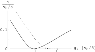
FIG. 1.: The spin gap $\Delta$ as a function of $g_{\scriptscriptstyle U}$; the solid line is for $g_{\scriptscriptstyle J}=v_{F}/5$ and the dashed line for $g_{\scriptscriptstyle J}=0$.

In summary, we have shown that a one-dimensional electron liquid weakly coupled by a spin-exchange interaction to a spin ladder with $Sn_{leg}\gg 1$ develops a spin gap. The gap exhibits a strong dependence on the sign and magnitude of the itinerant electron-electron interaction, but is insensitive to whether the coupling to the ladder is ferro- or antiferromagnetic. A symmetry argument implies that these results hold for any gapful ladder or gapless ladder with $Sn_{leg}\gg 1$. Applied to the striped phases seen in the cuprates this may suggest that the local antiferromagnetic correlations in the insulating domains may conspire with the electron correlations on the stripes to produce a sizeable spin gap. Details and extensions will be published elsewhere.

We wish to thank I. Affleck, S. A. Kivelson, A. A. Nersesyan, A. M. Tsvelik, and J. Voit for discussions and correspondence. H. J. acknowledges support from the Swedish Natural Science Research Council.

REFERENCES

• [1] For a recent review, see e.g. Proceedings of SCES98, to appear in Physica B.
• [2] J. M. Tranquada et al., Nature 375, 561 (1995) and references therein; Z.-X Shen et al. Science 280 259 (1998); P. Dai et al., Phys. Rev. Lett. 80, 1738 (1998); K. Yamada et al., Phys. Rev. B 57, 6165 (1998).
• [3] For a review, see J. Voit, Rep. Prog. Phys. 58, 977 (1995).
• [4] V. J. Emery, S. A. Kivelson and O. Zachar, Phys. Rev. B 56, 6120 (1997).
• [5] C. C. Tsuei and T. Doderer, to appear.
• [6] A. H. Castro Neto, C. de C. Chamon, and C. Nayak, Phys. Rev. Lett. 79, 4629 (1997).
• [7] L. Balents and M. P. A. Fisher, Phys. Rev. B 55, 11973 (1997).
• [8] A. E. Sikkema, I. Affleck and S. R. White, Phys. Rev. Lett. 79, 929 (1997).
• [9] M. Granath and H. Johannesson, unpublished.
• [10] See, for example, U. Lรถw et al., Phys. Rev. Lett. 72, 1918 (1994); J. Zaanen and O. Gunnarsson, Phys Rev B 40, 7391 (1989).
• [11] F. D. M. Haldane, Phys. Lett. A 93, 464 (1993).
• [12] S. Dellโ€™Aringa et al., Phys. Rev. Lett. 78, 2457 (1997).
• [13] D. V. Khveshchenko, Phys. Rev. B 50, 380 (1994).
• [14] In a Hamiltonian formulation of the nonlinear $\sigma$ model [18] $\mbox{\boldmath$n$}\!\times\!\partial_{t}\mbox{\boldmath$n$}$ is the angular momentum density which is equivalent to the ferromagnetic component $\ell$ in Eq. (5). Since $\ell$ is rapidly varying compared to $n$ it averages to zero over the length scales considered here.
• [15] For a review, see I. Affleck, in Fields, Strings and Critical Phenomena, edited by E Brรฉzin and J. Zinn-Justin (North-Holland, Amsterdam 1990).
• [16] I. Affleck and F. D. M. Haldane, Phys. Rev. B 36, 5291 (1987).
• [17] S. Chakravarty, Phys. Rev. Lett. 77, 4446 (1996).
• [18] For a review, see G. Sierra, in Proc. of the 1996 El Escorial Summer School on Strongly Correlated Magnetic and Superconducting Systems, (cond-mat/9610057).
• [19] S. Fujimoto and N. Kawakami, J. Phys. Soc. Jap. 63, 4322 (1994).
• [20] Recent work on the โ€œzig-zag chainโ€ used in the bosonization approach in [8] suggests that a massive phase may in fact appear also for ferromagnetic coupling (A. A. Nersesyan, A. O Gogolin and F. H. L. Essler, Phys. Rev. Lett. 81, 910 (1998)).