A measure of conductivity for lattice fermions
at finite density.

Abstract

We study the linear response to an external electric field of a system of fermions in a lattice at zero temperature. This allows to measure numerically the Euclidean conductivity which turns out to be compatible with an analytical calculation for free fermions. The numerical method is generalizable to systems with dynamical interactions where no analytical approach is possible.

PACS numbers: 11.15.Ha 71.10.Fd, 71.20.-b,

1 Introduction

The study of transport properties in a system of charged fermions is an interesting subject in areas as different as Physics of Plasma, Quantum Chromodynamics or Metals. In particular, the measure of the electrical conductivity is a very difficult and yet interesting problem, specially in presence of nonperturbative effects. In such a case, numerical methods are called for. In this work, we want to show that lattice-regularized Euclidean field theories can be useful in this respect, at least in the limit of vanishing temperature. However, it should be emphasized that the so called sign-problem needs still to be overcome in many cases [1] (see, though, Refs. [2, 3] for some successful simulations at finite density).

In this paper, we restrict ourselves to a model consisting of fermions that only interact with an external electromagnetic field. In spite of its simplicity, it shares many properties with more realistic models, and it can be considered as a necessary first step to check any numerical method which could be used in models with dynamical interactions. We consider the standard $U(1)$ lattice-action, with Wilson fermions and finite chemical potential, but with the gauge variables held fixed. We shall study the residue of the pole of the electrical conductivity at zero-frequency, which is purely imaginary. Since a non-vanishing value for this residue unambiguously signals a conducting phase, this is a rather interesting quantity in our opinion. In order to obtain it, we measure the electrical-current induced in the system by an external electric field. This technique requires a numerical calculation even in the case of an external spatially-homogeneous time-dependent electromagnetic field. The delicate point, however, is that our electric field varies in Euclidean time. One can nevertheless assume that there is a linear relation between the Euclidean current and the Euclidean electric field, at least for small fields. This Euclidean conductivity presents a pole whose residue can be straightforwardly measured. To check that the obtained result is physical, we follow a very elegant procedure due to Kohn[4]. He showed that the real-time residue can be measured by studying the sensitivity of the ground-state energy to an external Aharonov-Bohm electromagnetic field. We show how can this be done in the lattice formalism, and, in this particularly simple case of free fermions, we calculate it (unfortunately, the Kohn recipe seems really hard to use in a Monte Carlo study of a self-interacting problem). Although at present we lack a rigorous proof of the equivalence of both calculations, its excellent numerical agreement gives a strong support to the linear response method.

2 The Model

Let us consider a model of Wilson Fermions[5, 6] in a lattice of spacing $a_{\mathrm{s}}$ in the three spatial directions and $a_{\mathrm{t}}$ in the temporal one, coupled to an external electromagnetic field. We denote by $\lambda$ to the quotient $a_{\mathrm{t}}/a_{\mathrm{s}}$. The partition function can be written as (the $*$ superscript stands for complex conjugation) [7, 8, 9]

$${\mathcal{Z}}[U]=\int\prod_{z}\,{\mathrm{d}}\Psi_{z}{\mathrm{d}}\overline{\Psi}_{z}\exp\left[\sum_{x,y}\overline{\Psi}_{x}M_{xy}(U)\Psi_{y}\right]\,,$$ (1)

$$M_{xy}(U) = {\mathrm{e}}^{\lambda\mu}U_{x,0}(\gamma_{0}-r_{\mathrm{t}})\delta_{y,x+\hat{0}}-{\mathrm{e}}^{-\lambda\mu}U_{x,0}^{*}(\gamma_{0}+r_{\mathrm{t}})\delta_{y+\hat{0},x}$$

$$+ \lambda\sum_{i=1}^{3}[U_{x,i}(\gamma_{i}-r_{\mathrm{s}})\delta_{y,x+\hat{\imath}}-U_{x,i}^{*}(\gamma_{i}+r_{\mathrm{s}})\delta_{y+\hat{\imath},x}]+[(2m+6r_{\mathrm{s}})\lambda+2r_{\mathrm{t}}]\delta_{x,y}\ ,$$

where $U_{x,\nu}={\mathrm{e}}^{{\mathrm{i}A_{x,\nu}}}$, $A$ being the gauge field, and $\Psi_{x}$, $\overline{\Psi}_{x}$ are the anticonmuting Grassmann fermionic fields. The indices $x,y$ run on the points of the four-dimensional space-time lattice. We impose periodic boundary conditions for the gauge field, and periodic in space but antiperiodic in time ($\nu=0$) for the Grassmann field. The site $x+\hat{\nu}$ is the neighbor of $x$ in the $\nu=0,1,2,3$ direction. For finite temporal length, $L_{0}$, the system is at finite temperature $T=(a_{\mathrm{t}}L_{0})^{-1}$. In this paper we will only consider the zero temperature ($L_{0}\to\infty$) limit. We follow the prescription of introducing the chemical potential through an imaginary gauge field $A=(-{\mathrm{i}}\lambda\mu,0,0,0)$ [7, 8], which is fairly convenient for analytical calculations.

The Wilson parameter, $r$, can be taken different for the spatial and time directions. In the limit $\lambda\to 0$ with $a_{\mathrm{s}}$ fixed the model describes a spatial lattice with a continuous time (as electrons in a metal), while for a continuum field theory both spatial and time continuum limits should be taken.

We shall use the following representation for the (Euclidean) gamma matrices

$$\gamma_{0}=\left(\begin{array}[]{cc}0&1\\ 1&0\end{array}\right),\quad\gamma_{i}=\left(\begin{array}[]{cc}0&-{\mathrm{i}}\sigma_{i}\\ {\mathrm{i}}\sigma_{i}&0\end{array}\right),\$$ (3)

where $\sigma_{i}$ are the Pauli matrices.

To define the electric four-current in the lattice we recall that in the space-time continuum limit it is defined as

$$j_{\nu}(x)=\overline{\Psi}(x)\gamma_{\nu}\Psi(x)\,,$$ (4)

that can be obtained as a logarithmic derivative of the partition function respect to the gauge-field. This calculation can be exactly mimicked on the lattice noticing that a change in the link variable should be of the form $U_{x,\nu}\rightarrow{\mathrm{e}}^{{\mathrm{i}}\alpha_{x,\nu}}U_{x,\nu}$. In this way one obtains [8]:

$$\langle j_{x,\nu}\rangle={\mathrm{i}}\,\frac{\partial\log{\mathcal{Z}}}{\partial\alpha_{x,\nu}}\ ,$$ (5)

where now

$$\langle j_{x,0}\rangle = \left\langle\overline{\Psi}_{x}{\mathrm{e}}^{\lambda\mu}U_{x,0}(\gamma_{0}-r_{\mathrm{t}})\Psi_{x+\hat{0}}+\overline{\Psi}_{x+\hat{0}}{\mathrm{e}}^{-\lambda\mu}U_{x,0}^{*}(\gamma_{0}+r_{\mathrm{t}})\Psi_{x}\right\rangle\,$$ (6)

$$\langle j_{x,i}\rangle = \lambda\left\langle\overline{\Psi}_{x}U_{x,i}(\gamma_{i}-r_{\mathrm{s}})\Psi_{x+\hat{\imath}}+\overline{\Psi}_{x+\hat{\imath}}U_{x,i}^{*}(\gamma_{i}+r_{\mathrm{s}})\Psi_{x}\right\rangle\,,\ i=1,2,3\,.$$ (7)

The $j_{0}$ component is just the electric charge density that one encounters by differentiating with respect to $\lambda\mu$ the free energy density [8]. Moreover, from the gauge invariance of the determinant of the fermionic matrix, $M$, it is straightforward to prove the lattice continuity equation, for any configuration of the electromagnetic-field:

$$0=\sum_{\nu}\left(\langle j_{x,\nu}\rangle-\langle j_{x-\hat{\nu},\nu}\rangle\right)\,.$$ (8)

Eqs. (6) and (7) can be written free of Grassmann variables as

$$-\langle j_{x,0}\rangle = {\mathrm{e}}^{\lambda\mu}U_{x,0}\mathrm{Tr}[(\gamma_{0}-r_{\mathrm{t}})M^{-1}_{x+\hat{0},x}]+{\mathrm{e}}^{-\lambda\mu}U^{*}_{x,0}\mathrm{Tr}[(\gamma_{0}+r_{\mathrm{t}})M^{-1}_{x,x+\hat{0}}]\ ,$$ (9)

$$-\langle j_{x,i}\rangle = \lambda U_{x,i}\mathrm{Tr}[(\gamma_{i}-r_{\mathrm{s}})M^{-1}_{x+\hat{\imath},x}]+\lambda U^{*}_{x,i}\mathrm{Tr}[(\gamma_{i}+r_{\mathrm{s}})M^{-1}_{x,x+\hat{\imath}}]\ ,$$ (10)

where Tr stands for the trace over Dirac indices. The above expressions and the relation

$$M(U^{*})=\gamma_{1}\gamma_{3}\left(M(U)\right)^{*}\gamma_{3}\gamma_{1}\,,$$ (11)

allow to prove that

$$\langle j_{x,\nu}\rangle^{*}_{U}=\langle j_{x,\nu}\rangle_{U^{*}}\ .$$ (12)

In an uniform electrical field, the charge density should remain constant under field inversion, while the electrical current should change sign. Therefore, from Eq. (12) one expects the former to be real and the latter to be imaginary (Euclidean space-time!).

In absence of external fields ($U=1$) the matrix $M$ can be diagonalized in Fourier space, which allows to explicitly perform the functional integrals, and to compute the free energy and the propagator. For brevity, we only quote the result for the charge density in the case $r_{\mathrm{t}}=r_{\mathrm{s}}=1$, $\mu>0$, that in the infinite volume limit reads (see Refs. [10, 11] for similar calculations),

$$\rho(\lambda,\mu)=2\int_{-\pi}^{\pi}\frac{{\mathrm{d}}^{3}\mbox{\boldmath$k$}}{(2\pi)^{3}}\,\theta\left(\mu-\lambda^{-1}E(\mbox{\boldmath$k$})\right)\,,$$ (13)

where

$$E(\mbox{\boldmath$k$}) = \mathrm{arccosh}\left[\frac{1+\lambda^{2}\sum_{j}\sin^{2}k_{j}+\left(\lambda\Sigma(\mbox{\boldmath$k$})+1\right)^{2}}{2\left(\lambda\Sigma(\mbox{\boldmath$k$})+1\right)}\right]\,,$$ (14)

$$\Sigma(\mbox{\boldmath$k$}) = m+\sum_{j}\,(1-\cos k_{j})\ .$$ (15)

An useful quantity is the mechanical compressibility that, at zero-temperature coincides with the density of states:

$$\kappa(\lambda,\mu)=\frac{\partial\rho(\lambda,\mu)}{\partial\mu}=2\int_{-\pi}^{\pi}\frac{{\mathrm{d}}^{3}\mbox{\boldmath$k$}}{(2\pi)^{3}}\,\delta\left(\mu-\lambda^{-1}E(\mbox{\boldmath$k$})\right)=2\lambda\int_{E(\mbox{\scriptsize\boldmath$k$})=\lambda\mu}\frac{{\mathrm{d}}^{2}S}{(2\pi)^{3}}\,\frac{1}{\left\|\mbox{\boldmath$\nabla_{k}$}E(\mbox{\boldmath$k$})\right\|}\,.$$ (16)

The density of states of the system present a typical band structure (see the upper part of Fig. 1, dashed line). The upper limit of the band corresponds to the saturation due to the Fermi statistics (one particle per lattice-site). Since the function $E(\mbox{\boldmath$k$})$ is periodic, its gradient has zeroes in the Brillouin zone, producing non-analiticies as the cusps in Fig. 1 (the so-called Van-Hove singularities [12]).

Figure 1: Density of states (upper part) and residue of the conductivity (lower part) for $\mu>0$. The dashed lines correspond to analytical calculations in Fourier space (see Eqs. (13), (16), and (24)). The solid lines are obtained numerically in finite lattices (see section 4). In all cases $r=1$.

3 The Electrical Conductivity

In a classical paper, Kohn [4] developed an elegant characterization of a conductor, at zero temperature. His method allows the measurement of the following limit for the imaginary part of the electrical conductivity, $\sigma^{\prime\prime}$,

$$Z=\lim_{\omega\to 0}\omega\sigma^{\prime\prime}(\omega)\ .$$ (17)

If this limit turns out to be non zero, the system is a conductor. The construction is as follows. The system of interest is constrained to verify periodic boundary conditions in the (say) first spatial direction, and immersed in an Aharonov-Bohm like electromagnetic field $A=(0,\alpha,0,0)$. With this choice of boundary conditions the product $L_{1}a_{\mathrm{s}}\alpha$ is gauge invariant since it represents the magnetic flux traversing the system. It can be shown that

$$Z=-\frac{1}{V_{\mathrm{s}}}\left.\frac{\mathrm{d}^{2}E_{0}}{\mathrm{d}\alpha^{2}}\right|_{\alpha=0}\,,$$ (18)

where $E_{0}$ is the ground-state energy and $V_{\mathrm{s}}$ is the spatial volume. It is crucial that the infinite limit volume is taken after the $\alpha$ derivative is performed, since the effect of the Aharonov-Bohm field can be thought of as a change in the boundary conditions (see below). In the infinite volume limit, the energy no longer depends on $\alpha$.

In our case, as the free energy and the ground-state energy coincide in the zero temperature limit, we can study the residue in the following way

$$Z=-\lim_{V_{\mathrm{s}}\to\infty}\lim_{T\to 0}\left.\frac{\mathrm{d}^{2}\tilde{f}}{\mathrm{d}\alpha^{2}}\right|_{\alpha=0}\,,$$ (19)

where $\tilde{f}$ is obtained from the intensive free energy $f$ after subtracting the vacuum contribution: $\tilde{f}(\mu)=f(\mu)-f(0)$.

Let us sketch the calculation. The free energy should be calculated in a finite volume and at finite temperature. We introduce our system in the Aharonov-Bohm electromagnetic field:

$$U_{x,0}=U_{x,2}=U_{x,3}=1\ ,\ U_{x,1}={\mathrm{e}}^{{\mathrm{i}}\alpha}\,.$$ (20)

This field can be transformed into a boundary effect by performing the following gauge transformation:

$$U_{x,\nu}\rightarrow U^{\mathrm{G}}_{x,\nu}={\mathrm{e}}^{{\mathrm{i}}g(x)}\,U_{x,\nu}{\mathrm{e}}^{-{\mathrm{i}}g(x+\hat{\nu})}\,\ ,\ g(x)=\alpha x_{1}\,,$$ (21)

so that $U^{\mathrm{G}}=1$ excepting

$$U^{\mathrm{G}}_{(x_{1}=L_{1}-1),1}={\mathrm{e}}^{{\mathrm{i}}\alpha L_{1}}\,.$$ (22)

By direct inspection of the fermion matrix in Eq. (2), one can easily recognize that a system verifying periodic boundary conditions in the 1 direction in the field $U^{\mathrm{G}}$ is equivalent the same system with no field at all, but verifying

$$\Psi(x_{0},x_{1}+L_{1},x_{2},x_{3})={\mathrm{e}}^{{\mathrm{i}}\alpha L_{1}}\Psi(x_{0},x_{1},x_{2},x_{3})\ ,$$ (23)

This amounts to substituting $k_{1}$ by $k_{1}+\alpha$ in the momentum-quantification in a finite lattice. For a system of free fermions the free energy can be now straightforwardly calculated. Once the $\alpha$ derivative is performed, the zero temperature limit can be taken by transforming the $k_{0}$ sum into an integral. We get, in the simplest case $r_{\mathrm{t}}=r_{\mathrm{s}}=1$, $\mu>0$,

$$Z=-2\int_{-\pi}^{\pi}\frac{\mathrm{d}^{3}\mbox{\boldmath$k$}}{(2\pi)^{3}}\frac{\partial^{2}E(\mbox{\boldmath$k$})}{\partial k_{1}^{2}}\theta(\mu-\lambda^{-1}E(\mbox{\boldmath$k$}))\,.$$ (24)

Notice that for the empty system, $\mu<\lambda^{-1}E_{\mathrm{min}}$, the integral vanishes, as well as for the full band $\mu>\lambda^{-1}E_{\mathrm{max}}$, since $E(\mbox{\boldmath$k$})$ is a periodic function of $k_{1}$. The three dimensional integrals (24) can be performed using a Monte Carlo method. The results are shown in Fig. 1 (dashed line in the lower part).

4 Numerical Calculations

In this section, we are going to reproduce the results of the sections 2 and 3 by directly considering the integration of the partition function. This method has the advantage of being generalizable to inhomogeneous external fields, and also when interacting dynamical fields are present. Examples of how to introduce an external field on an interacting lattice-gauge system can be found in Refs. [13]. To compute the partition function it is necessary to work in finite lattices, consequently, an infinite volume limit should be taken.

We have carried out measures in symmetric lattices of sizes $L=4,6,8,10,12,14$ and $16$, with $m=1/2$ and $\lambda=1$. For the hopping term, we have taken $r_{\mathrm{s}}=r_{\mathrm{t}}=1$. As the integral in the fermionic fields is Gaussian, the computation of the electric current just requires the inversion of a $4V$ matrix, $V$ being the space-time volume. The fermion matrix (2) being sparse, we have used a conjugate-gradient algorithm for the numerical inversion.

We first consider the density of states in a vanishing external field. In order to measure $\partial\rho/\partial\mu$ we invert the matrix at $\mu\pm\epsilon$ for $\epsilon$ small enough. In interacting systems the derivative can be calculated in terms of connected correlation-functions [10].

The numerical results are plotted in Fig. 1, upper part, together with the infinite volume values obtained analytically. Although the finite size effects are non negligible even in the larger lattices for most values of $\mu$, there is a clear trend to the asymptotic values.

Unfortunately, for an interacting system it is not immediate how to implement Kohn’s method for calculating the residue of the conductivity. In fact, the free energy is rather hard to calculate with a Monte Carlo simulation and what one directly obtains are mean-values. We are now going to present a different way of computing the residue, by directly measuring the system response to an external electrical field. Notice that the presence of an electric field requires a non-homogeneous vector potential and consequently the inversion of the fermion matrix can no longer be performed in closed analytical form. This new recipe can be straightforwardly generalized to interacting systems, but its equivalence with the Kohn’s method is just an ansatz. Nevertheless the agreement is excellent, as we will show.

By analogy with continuum electrodynamics, we want to study the electric current induced in the system by an external weak uniform electric field in the $1$ direction. The conductivity (in the frequency domain), will be the proportionality constant between the electrical current and the external field.

There are some subtleties that need to be considered when putting an external electric field on the lattice. We take the gauge-field configuration ($t=x_{0}$)

$$U_{x,0}={\mathrm{e}}^{{\mathrm{i}}\,{\mathcal{E}}_{t}x_{1}},\quad U_{x,i}=1\,,$$ (25)

$${\mathcal{E}}_{t}=\frac{2\pi}{L_{1}}n_{t}\ ,\quad n_{t}\in\left\{-\frac{L_{1}}{2},-\frac{L_{1}}{2}+1,\ldots,\frac{L_{1}}{2}-1,\frac{L_{1}}{2}\right\}\,.$$ (26)

Notice that the quantization of the electric-field is due to the spatial boundary conditions. To preserve the translational symmetry, the displaced gauge field

$$U_{x,0}={\mathrm{e}}^{{\mathrm{i}}\,{\mathcal{E}}_{t}(x_{1}-\xi)}\ ,\quad\xi\ \mathrm{integer}\ ,$$ (27)

should be a gauge-transform of the one in Eq. (25). Since the needed gauge transformation is analogous to Eq. (21), it is easy to check that the condition that allows this transformation is the trivialness of the Polyakov loop:

$$\prod_{t=0}^{L_{0}-1}U_{(t,\mbox{\scriptsize\boldmath$x$}),0}=1\quad\mathrm{or}\quad\sum_{t=0}^{L_{0}-1}{\mathcal{E}}_{t}=2\pi n\,,$$ (28)

with $n$ integer. This condition also allows to transform the gauge field to the Coulomb gauge $A_{0}=0$. If condition (28) is violated, the translational invariance is lost and the electric current is no longer spatially homogeneous even on a homogeneous electric-field. However, with the correct field choice (28), we get a homogeneous electrical current aligned with the external electrical field, and imaginary as anticipated in Eq. (12). In order to directly compare with the results obtained with Eq. (24), let us define

$$j(t)={\mathrm{i}}\langle j_{x,1}\rangle$$ (29)

If we want to stay within linear-response theory, we have to postulate a linear relation between the Fourier transform of the electrical current $j(t)$ and the external electrical field ${\mathcal{E}}_{t}$:

$$\hat{\jmath}(\omega)=\sigma(\omega)\hat{\mathcal{E}}(\omega)\,.$$ (30)

Notice that both $j(t)$ and ${\mathcal{E}}_{t}$ being real, $\sigma(-\omega)=\sigma^{*}(\omega)$. However, the results can be more cleanly cast in terms of a modified Fourier transform for the electrical field:

$${\tilde{\mathcal{E}}}(\omega)=\frac{1}{\sqrt{L_{0}}}\sum_{t=0}^{L_{0}-1}{\mathcal{E}}_{t}{\mathrm{e}}^{-{\mathrm{i}}\omega(t+1/2)}\,.$$ (31)

The rationale for this is that the electrical field ${\mathcal{E}}_{t}$ on the lattice lives mid-way between sites at times $t$ and $t+1$. The modified conductivity $\tilde{\sigma}(\omega)=\hat{\jmath}(\omega)/{\tilde{\mathcal{E}}}(\omega)$ is related with the previous one by

$$\tilde{\sigma}(\omega)=\sigma(\omega){\mathrm{e}}^{{\mathrm{i}}\omega/2}\,.$$ (32)

The nice feature of $\tilde{\sigma}(\omega)$ is that it turns out to be purely imaginary.

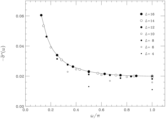
Figure 2: The imaginary part of the conductivity $\tilde{\sigma}(\omega)$ of a system of free Wilson fermions at $r=1$ , $m=1/2$ and $\mu=1$.

In Fig. 2 we plot the imaginary part of $\tilde{\sigma}(\omega)$ as obtained from a field with $n_{0}=1$ and $n_{1}=-1$, (from now on we shall only indicate the non-vanishing $n_{i}$’s), in a system of Wilson fermions with $m=1/2$, $r=1$ and $\mu=1$, that is within the band energy-range and therefore with a non-vanishing Fermi surface. We see that for large frequencies the thermodynamic limit is reached in rather small lattices. However, at the minimal reachable frequency ($2\pi/L_{0}$) the conductivity is rapidly growing suggesting a singularity at zero frequency. In fact, for a (classical) system of free particles of density $n$ we expect that $\sigma(\omega)$ will behave as

$$\sigma^{\mathrm{free,classical}}\sim\ -{\mathrm{i}}\ \frac{e^{2}n}{m\,\omega}\,.$$ (33)

Notice that if $\sigma(\omega)$ has a pole at $\omega=0$ with a purely imaginary residue the same will hold true for $\tilde{\sigma}(\omega)$, and both residues will be equal. Although the Euclidean conductivity $\tilde{\sigma}(\omega)$ do not match the real-time one (being imaginary, it cannot fulfill the Kramers-Kronig relations), one can formally expect the residues to coincide in the passage from $\omega$ to ${\mathrm{i}}\omega$. This suggest to define the following quantity which will be the basic object of our study:

$$Z^{\mathrm{E}}=\frac{1}{i}\omega^{\mathrm{min}}\tilde{\sigma}(\omega^{\mathrm{min}})\,,\quad\omega^{\mathrm{min}}=\frac{2\pi}{L_{0}}\,.$$ (34)

In the $L_{i},L_{0}\to\infty$ limit, $Z^{\mathrm{E}}$ tend to the residue of the pole. In order to measure this, we have considered the smallest of possible external disturbances: $\{n_{0}=1,n_{L_{0}/2}=-1\}$.

Figure 3: The Fourier transform at zero frequency of the electrical current as a function of the inverse lattice size.

Our result is shown in Fig. 1, lower part. We see that the Euclidean residue follows quite closely Kohn’s result, which in fact can be considered as the infinite volume limit for our calculation. Moreover, the physical picture is rather transparent: when the band is full, the system gets almost inert, while when the band is empty, it can be excited by the external field creating a hole in the Dirac sea. Since the smallest possible excitation has frequency $2\pi/L_{0}$, to be compared with a gap $2m$, it is reasonable that at $\mu=0$, the larger is the space-time lattice, the smaller is the system response. In fact, notice that in Fig. 1 when $\mu$ is below the lower band limit, the curves get horizontal: in this range of $\mu$ the system can be only excited by crossing the gap between the Dirac sea and the conduction band. And the gap is, of course, $\mu$ independent in a non-interacting system.

We remark that our results have been found within the linear response approximation. We can control this approximation in several ways. One is to study the Fourier transform of the current, for frequencies at which the Fourier transform of the external-field vanishes. In Fig. 3 we show the zero-mode of the electrical current for the electrical-field $\{n_{0}=1,n_{1}=-1\}$. We see that this non-linear effect tends to zero with growing lattice-size, which is quite reasonable since the minimum possible electric field is $2\pi/L_{1}$. The non-linear corrections are oscillating, but modulated by a rapidly decaying function. Roughly speaking, for the largest lattice the non linear effects are of the same order as the distance to the thermodynamic limit. A further check can be done by comparing the residue obtained from the data in Fig. 2 with the one in Fig. 1: in the $L=14$ lattice, the differences are at the $0.3\%$ level, while in the $L=6$ lattice the differences are at the $1.6\%$ level. Therefore, we believe that non-linear effects are under control for the not too small fields that we can deal with.

5 Conclusions

We have presented a simple way of studying the electrical conductivity of a system of Wilson fermions at finite density and zero-temperature in a path-integral formalism. In particular, we have computed the residue of the zero frequency pole of the conductivity, by numerically considering the linear response to an external electric field, varying in Euclidean time. The results have been contrasted with an analytical computation based on a method proposed by Kohn, and an excellent agreement has been found. As a further cross-check, we have computed the density of states both analytically and numerically in a finite lattice, obtaining a nice thermodynamic limit convergence. It should be emphasized that in contrast with the analytical calculation which can only be done for a non interacting system (or, at most, for simple external fields), the numerical calculations are easily generalizable to more complex models, as fermions self-coupled with quartic interactions or via a dynamic bosonic field.

An open, very interesting question is the possibility of extracting the full real-time electrical conductivity function from its Euclidean counterpart. We have shown that the residue of the zero-frequency pole can indeed be obtained. It would be also very interesting to extend this approach to systems at finite-temperature.

6 Acknowledgements

This work was triggered during a discussion with F. Guinea to whom we are indebted for many suggestions, discussions and bibliographical help. The numerical calculations have being carried-out in the RTNN machines at the universities of Zaragoza and Complutense de Madrid. This work has been partially supported by CICYT, contracts AEN97-1680,1693,1708.

References

- [1] F. Karsch, M-P. Lombardo (editors), QCD at Finite Barion Density, Nucl. Phys. A642(1998) Proc. Supp. 1-2.
- [2] F. Karsch, J.B. Kogut, H.W. Wyld, Nucl. Phys. B280[FS18](1987)289; S.J. Hands, A. Kocić, J.B. Kogut, Nucl. Phys. B390(1993)355; S.J. Hands, S. Kim, J.B. Kogut, Nucl. Phys. B442(1995)364; I. Barbour, S. Hands, J.B. Kogut, M-P. Lombardo, S. Morrison, Nucl. Phys. B557(1999)327.
- [3] M.P. Lombardo, preprint hep-lat/9907025; S. Hands, J.B. Kogut, M.P. Lombardo, S. Morrison, Nucl. Phys. B558(1999)327.
- [4] W. Kohn, Phys. Rev. 133(1964)A171.
- [5] K.G. Wilson, Phys. Rev. D14(1974)2455.
- [6] K.G. Wilson. Quarks and Strings on the Lattice, in New Phenomena in subnuclear Physics. Editor A. Zichichi. Plenum Press, New York 1977.
- [7] P. Hasenfratz, F. Karsch, Phys. Lett. B125(1983)308.
- [8] J.B. Kogut, H. Matsuoka, M. Stone, H.W. Wyld, S. Shenker, J. Shigemitsum D.K. Sinclair, Nucl. Phys. B225[FS9](1983)93.
- [9] I. Bender, H.J. Rothe, I.O. Stomatescu, W. Wetzel, Z. Phys. C58(1993)333.
- [10] I. Montvay, G. Münster, Quantum Fields on a Lattice. Cambridge Univ. Press. 1994.
- [11] R.V. Gavai, Phys. Rev. D32(1985)519.
- [12] N.W. Ashcroft and N.D. Mermin, Solid State Physics, Saunders College Publishing, 1976.
- [13] G. Martinelli, G. Parisi, R. Petronzio, F. Rapuano, Phys. Lett. 116B (1982) 434; C. Bernard, T. Draper, K. Olynyk, M. Rushton, Phys. Rev. Lett. 49 (1982) 1076; J. Ambjorn, V.K. Mitryushkin, V. G. Bornyakov, A. M. Zadorozhnyi, Phys. Lett. B225 (1989) 153; M. Lüscher, P. Weisz, R. Sommer, U. Wolff, Nucl. Phys. B389 (1993) 247.