Exact statistical properties of the Burgers equation

Abstract

The one dimensional Burgers equation in the inviscid limit with white noise initial condition is revisited. The one- and two-point distributions of the Burgers field as well as the related distributions of shocks are obtained in closed analytical forms. In particular, the large distance behavior of spatial correlations of the field is determined. Since higher order distributions factorize in terms of the one and two points functions, our analysis provides an explicit and complete statistical description of this problem.

I Introduction

The Burgers equation for the velocity field $u(x,t)$

$${\partial\over\partial t}u(x,t)+u(x,t){\partial\over\partial x}u(x,t)=\nu{\partial^{2}\over\partial x^{2}}u(x,t)$$ (1)

has recently raised much interest because of its multiple connections to a variety of physical and mathematical problems. Background and references can be found for instance in the recent book [1]. The original Burgers problem [2] concerned the statistics of the velocity field $u(x,t)$ and of shock-waves in the inviscid limit $\nu\to 0$ when the distribution of the initial velocity field $u(x,0)$ is a $\delta$-correlated Gaussian (white noise). It provides an over-simplified, but analytically tractable model of turbulence which has attracted a lot of studies over the last decades. In [2] a considerable amount of work is done to calculate various moments of these distributions, but the distributions themselves were not obtained in closed forms due to the complexity of the analysis. The question has been addressed again by Tatsumi and Kida [3] and Kida [4]. In [3], kinetic equations for the dynamics of shocks are used to derive scaling properties of the distributions, and in the second part of [4], Kida presents the result of numerical simulations for the distribution of the strength and the velocity of shocks. Recently, Avellaneda and E [5] and Avellaneda [6] have derived rigorous upper and lower bounds of the cubic type $\exp(-Cu^{3})$ for the tails of the one-point distribution. Such cubic bounds have also been obtained in [7] for the distribution of mass in the closely related problem of ballistic aggregation.

In this work we revisit Burgers problem by providing closed analytical forms of the statistical distributions for the field and the associated distributions of shock-waves. Our main contributions are a simple formulae expressing the one-point distribution as integrals over the analytic continuation of the Airy function on the imaginary axis (formulae (74) and (81)) as well as a detailed study of the clustering behavior of the two-point distributions. Since it is known that $u(x,t)$ as a function of $x$ (for fixed $t$) is a Markov process [5], the higher order distributions factorize in products of one and two-point functions. Hence our results give a complete solution to the one dimensional Burgers problem with initial white noise distributed data in the inviscid limit.

In section II, we recall well known facts about the Burgers equation in the inviscid limit with the purpose to introduce the notations and the definitions of the one- and two-point distribution functions. In section III, using the notion of first hitting time, these distributions are expressed in terms of the basic propagator for a Brownian motion constrained by parabolic barriers. It appears that all statistical properties of the Burgers problem are embodied in the knowledge of three functions called here $I$, $J$ and $H$. The functions $I$ and $J$ are calculated in section IV and the one-point distribution of fields and shocks are discussed. In particular an explicit formula for the strength distribution is obtained. These results have already been announced in [8] in the equivalent language of ballistic aggregation. The section V is entirely devoted to the study of the large distance behavior of the two-point distribution (the function $H$). Since the analysis is somewhat heavy, technical parts have been relegated in appendices. Finally the factorization of higher order distributions as well as their time dependence are discussed in the conclusion.

The situation considered by Burgers is particularly relevant to the non equilibrium statistical model of ballistic aggregation: it is known [2, 4] that the dynamics of shocks in Burgers turbulence is closely related to the dynamics of the aggregating particles. White noise initial distribution of the Burgers velocity field corresponds to uncorrelated Maxwellian initial velocity distribution of the particles undergoing aggregation. Hence our results also solve this statistical mechanical model. A precise connection between the two problems can only be made in a proper scaling limit since ballistic aggregation always retains the discrete nature of particles whereas Burgers velocity field describes a continuous medium. This connection will be discussed in an other paper [9]. Notice also that the Burgers equation is equivalent to the KPZ equation [10] of surface growth processes with the height $h$ of the surface given by $u(x,t)=\partial_{x}h(x,t)$. Burgers turbulence arising from other classes of stochastic initial data (see e.g. [11]) or from the action of external random forces (see e.g. [12]), which is the subject of considerable current investigations, is not discussed in this paper.

II General setting

For convenience, we shortly recall the construction of solutions of the Burgers equation in the inviscid limit, see [2], [1] and references therein. Introducing the potential $\partial\Psi(x,t)/\partial x=u(x,t)$ together with the Hopf-Cole transformation

$$\Psi(x,t)=-2\nu\ln\theta(x,t),$$ (2)

one finds that the function $\theta(x,t)$ satisfies the linear diffusion equation

$${\partial\over\partial t}\theta(x,t)=\nu{\partial^{2}\over\partial x^{2}}\theta(x,t).$$ (3)

It can be readily solved leading to the explicit solution

$$u(x,t)={\int_{-\infty}^{\infty}dy{x-y\over t}\exp\left(-{1\over 2\nu}F(x,y,t)\right)\over\int_{-\infty}^{\infty}dy\exp\left(-{1\over 2\nu}F(x,y,t)\right)}$$ (4)

where

$$F(x,y,t)={(x-y)^{2}\over 2t}-\psi(y)$$ (5)

with

$$\psi(y)=-\Psi(y,0)=-\int_{0}^{y}dy^{\prime}\,u(y^{\prime},0)$$ (6)

which depends upon the initial condition. Burgers turbulence corresponds here to the situation where the initial velocity field $u(x,0)$ is a white noise process in space, or equivalently $\psi(y)$ is a two-sided Brownian motion pinned at $\psi(0)=0$.

In the inviscid limit $\nu\to 0$, the only contributions of the integrals in Eq.(4) come from the minima of the function $F(x,y,t)$, which depend on the initial condition through $\psi(y)$,

$$\xi(x,t)=\min_{y}F(x,y,t)$$ (7)

and we obtain

$$u(x,t)={x-\xi(x,t)\over t}.$$ (8)

Due to the scaling properties of the solution $u(x,t)$, one can trivially take into account the time dependence of the problem. Indeed the scaled Brownian motion $t^{\alpha/2}\psi(yt^{-\alpha})$ is equivalent in probability to $\psi(y)$ so that by (7) and (8) with $\alpha=2/3$ one has that $t^{2/3}\xi\left({x\over t^{2/3}},1\right)$ is equivalent to $\xi(x,t)$ and $t^{-1/3}u\left({x\over t^{2/3}},1\right)$ is equivalent to $u(x,t)$. We study from now on the fixed time $t=1$ solution $u(x,1)\equiv u(x)$. It will then always be possible to recover the time-dependent solution through this scaling property as we shall see in the concluding section.

The minimum $\xi(x)\equiv\xi(x,1)$ as a function of $x$ can be found with the help of a nice geometrical interpretation of the solution. One considers a realization of the Brownian motion $\psi(y)$ and a parabola centered at $x$ of equation $(x-y)^{2}/2+C$ (see Fig.1) and adjusts the constant $C$ in order for the parabola to touch $\psi(y)$ without ever crossing it. The coordinate of the contact point is the minimum $\xi(x)$ leading thus to $u(x)=x-\xi(x)$. Then one glides the parabola on the graph of $\psi(y)$ by a continuous change of its center $x$ and $C$ until it touches it for $x=x_{i}$ on two contact points $\xi_{i}$ and $\xi_{i+1}$. Thus at $x=x_{i}$, the function $F(x,y,1)$ has two minima leading to a discontinuity of $u(x)$, called a shock, where $\lim_{\epsilon\to 0}u(x_{i}-\epsilon)=x_{i}-\xi_{i}$ and $\lim_{\epsilon\to 0}u(x_{i}+\epsilon)=x_{i}-\xi_{i+1}$. To make $u(x)$ singled valued at a shock, we define it to be continuous from the left setting $u(x_{i})=x_{i}-\xi_{i}$.

A shock is characterized (see Fig.1) by its location $x_{i}$ and two parameters which can be taken as

$$\mu_{i}=\xi_{i+1}-\xi_{i}\;\;\;\;{\rm"strength"},\;\;\;\;\nu_{i}=x_{i}-\xi_{i}\;\;\;\;\;{\rm"wavelength"}.$$ (9)

Instead of $\nu_{i}$ it will also be convenient to use the parameter $\eta_{i}$

$$\eta_{i}=\frac{\mu_{i}^{2}}{2}-\mu_{i}\nu_{i},\;\;\;\;\nu_{i}=\frac{\mu_{i}}{2}-\frac{\eta_{i}}{\mu_{i}}.$$ (10)

FIG. 1.: Geometrical interpretation of the solution $u(x)=x-\xi(x)$ for a given realization of the Brownian motion $\psi(y)$ which stays below a parabola of equation $s(y)=(y-x_{i})^{2}/2+C$ but on two contact points $\psi(\xi_{i})=(\xi_{i}-x_{i})^{2}/2+C$ and $\psi(\xi_{i+1})=(\xi_{i+1}-x_{i})^{2}/2+C$. A shock is located at $x_{i}$ with strength $\mu_{i}=\xi_{i+1}-\xi_{i}$ and wavelength $\nu_{i}=x_{i}-\xi_{i}$ while $\eta_{i}=\mu_{i}^{2}/2-\mu_{i}\nu_{i}$.

The quantities of interest to be computed are on one hand the joint distribution densities $p_{n}(x_{1},u_{1};x_{2},u_{2};\ldots;x_{n},u_{n})$ for the Burgers velocity field to have values in-between $u_{1}$ and $u_{1}+du_{1}$, $\ldots$ , $u_{n}$ and $u_{n}+du_{n}$ at points $x_{1},\ldots,x_{n}$, when average is taken over the realizations of the initial condition $u(x,0)$. On the other hand we will also consider the joint distribution densities of shocks $\rho_{n}(x_{1},\mu_{1},\eta_{1};x_{2},\mu_{2},\eta_{2};\ldots;x_{n},\mu_{n},\eta_{n})$. We shall obtain the joint distribution for the Burgers velocity field $u(x)$ from that of the variable $x-\xi(x)$. At time $t=1$, these two sets of variables coincide and we identify both distributions.

Consider first the one-point distribution density $p_{1}(x,u)$ where $u(x)=x-\xi(x)=u$. Because of translation invariance, $p_{1}(x,u)=p_{1}(0,u)\equiv p_{1}(u)$ and $u(0)=-\xi(0)=u$. Hence $p_{1}(u)$ is the measure of the set of all Brownian paths $\psi(y)$ with $\psi(0)=0$ that have their first contact (f.c.) with a parabola $y^{2}/2+C$ at $\xi(0)=-u$. As one can set the origin of coordinates to be at this contact point, it is given by the measure

$$p_{1}(u)=E\{\psi(y)\leq s_{u}(y),y\in R;\;\;{\rm f.c.\;with\;}s_{u}(y)\;{\rm at}\;(0,0)\}$$ (11)

of the set of paths that stay below the parabola

$$s_{u}(y)=\frac{y^{2}}{2}-uy$$ (12)

and have their first contact with it at $\psi(0)=0$. By first contact in (11), we mean that the path is strictly below the parabola $\psi(y)<s_{u}(y)$ for $y<0$, is assigned to pass at $\psi(0)=0$ and is then such as $\psi(y)\leq s_{u}(y)$ for $y\geq 0$. The expectation $E\{\cdots\}$ refers to Brownian paths running in the infinite “time” interval $-\infty<y<\infty$.

Likewise, the two-point joint density distribution $p_{2}(0,u_{1};x,u_{2})\equiv p_{2}(x,u_{1},u_{2})$ is the measure of the set of paths with $\psi(0)=0$ that have a first contact with a parabola $y^{2}/2+C_{1}$ (centered at the origin) at $\xi(0)=-u_{1}$ and a first contact with a second parabola $(y-x)^{2}/2+C_{2}$ (centered at $x$) at $\xi(x)=x-u_{2}$. Once again, we fix the origin at the contact point with the first parabola. Thus $p_{2}(x,u_{1},u_{2})$ is the measure of the set of paths which stay below both the parabolas $s^{(1)}(y)=s_{u_{1}}(y)$ centered at $u_{1}$ and a second parabola $s^{(2)}(y)$ centered at $x+u_{1}$ of equation $(y-x-u_{1})^{2}/2+C$, while the paths have a first contact point $\psi(0)=0$ with $s^{(1)}(y)$ and a first contact point $\psi(x+u_{1}-u_{2})=q$ with $s^{(2)}(y)$, where $x>0$, $x+u_{1}-u_{2}>0$, see Fig. 2 . In terms of this parameter $q$ the equation of the second parabola is

$$s^{(2)}(y)=\frac{(y-x-u_{1})^{2}}{2}-\frac{u_{2}^{2}}{2}+q$$ (13)

Now, $q$ is arbitrary except for the constraints that the first contact point with $s^{(1)}(y)$ must be below the second parabola, namely $s^{(2)}(0)\geq 0$, and that the first contact point with $s^{(2)}(y)$ must be below the first parabola, namely $s^{(1)}(x+u_{1}-u_{2})\geq q$. This leads to the condition $-q_{1}\leq q\leq q_{2}$ with

$$q_{1}=q_{1}(x,u_{1},u_{2})=\frac{1}{2}(x+u_{1}-u_{2})(x+u_{1}+u_{2}),\quad q_{2}=q_{2}(x,u_{1},u_{2})=\frac{1}{2}(x+u_{1}-u_{2})(x-u_{1}-u_{2}).$$ (14)

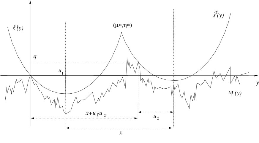
FIG. 2.: Brownian interpretation of the two-point distribution of the velocity field $p_{2}(x,u_{1},u_{2})$. The Brownian paths stays under the parabolas $s^{(1)}(y)=y^{2}/2-u_{1}y$ and $s^{(2)}(y)=(y-x-u_{1})^{2}/2-u_{2}^{2}/2+q$ but on two contact points $\psi(0)=0$ and $\psi(x+u_{1}-u_{2})=q$ where $-(x+u_{1}-u_{2})(x+u_{1}+u_{2})/2\leq q\leq(x+u_{1}-u_{2})(x-u_{1}-u_{2})/2$.

Hence

$$p_{2}(x,u_{1},u_{2})=E\left\{\psi(y)\leq s^{(1)}(y),\;\psi(y)\leq s^{(2)}(y),\;y\in R;\right.$$ (15)

$$\quad\quad\left.{\rm f.c.\;with}\;s^{(1)}(y)\;{\rm at}\;(0,0),\;{\rm f.c.\;with}\;s^{(2)}(y)\;{\rm at}\;(x+u_{1}-u_{2},q),\;-q_{1}\leq q\leq q_{2}\right\}.$$ (16)

The distributions $p_{1}(u_{1})$ and $p_{2}(x,u_{1},u_{2})$ have the normalizations

$$\int_{-\infty}^{\infty}du_{1}\,p_{1}(u_{1})=1$$ (17)

and

$$\int_{-\infty}^{\infty}du_{2}\,p_{2}(x,u_{1},u_{2})=p_{1}(u_{1}),\quad\lim_{x\to 0}p_{2}(x,u_{1},u_{2})=\delta(u_{1}-u_{2})$$ (18)

The distribution of shocks are defined in the same manner. By translation invariance $\rho_{1}(x,\mu,\eta)=\rho_{1}(0,\mu,\eta)\equiv\rho_{1}(\mu,\eta)$ is independent of $x$. It is given by the measure of the set of paths that have two contacts with the parabola $s_{\nu}(y)=y^{2}/2-\nu y$ (recall that $\nu=\frac{\mu}{2}-\frac{\eta}{\mu}$), a first contact at $\psi(0)=0$ and a last contact (l.c.) at $\psi(\mu)=\eta$, (see Fig. 1)

$$\rho_{1}(\mu,\eta)=E\left\{\psi(y)\leq s_{\nu}(y),\,y\in R;\;{\rm f.c.\;with}\;s_{\nu}(y)\;{\rm at}\;(0,0);\;{\rm l.c.\;with}\;s_{\nu}(y)\;{\rm at}\;(\mu,\eta)\right\}.$$ (19)

The joint distribution $\rho_{2}(0,\mu_{1},\eta_{1};x,\mu_{2},\eta_{2})$ of two shocks at distance $x$ is the set of paths that have two contacts with the parabola $s_{\nu_{1}}(y)$ as above and two contacts with an other parabola whose characteristics will be given in the next section. Notice that the centers of the two parabolas are separated by a distance $x$.

All quantities will be eventually expressed in terms of the transition probability kernel for Brownian motion in presence of parabolic absorbing barriers [13, 14]. Consider the conditional probability density $K_{\nu}(\mu_{1},\eta_{1},\mu_{2},\eta_{2})$ for the Brownian motion $\psi(y)$, starting from $\psi(\mu_{1})=\eta_{1}$, to end at $\psi(\mu_{2})=\eta_{2}$ while staying under the barrier $\psi(y)<s_{\nu}(y)=y^{2}/2-\nu y$ for $\mu_{1}\leq y\leq\mu_{2}$

$$K_{\nu}(\mu_{1},\eta_{1},\mu_{2},\eta_{2})=E_{\mu_{1},\eta_{1}}\left\{\psi(y)<s_{\nu}(y),\,\mu_{1}\leq y\leq\mu_{2};\;\psi(\mu_{2})=\eta_{2}\right\}.$$ (20)

It thus satisfies the diffusion equation

$$\partial_{\mu_{2}}K_{\nu}(\mu_{1},\eta_{1},\mu_{2},\eta_{2})={D\over 2}\partial_{\eta_{2}}^{2}K_{\nu}(\mu_{1},\eta_{1},\mu_{2},\eta_{2})$$ (21)

with $K_{\nu}(\mu,\eta_{1},\mu,\eta_{2})=\delta(\eta_{1}-\eta_{2})$ and $K_{\nu}(\mu_{1},s_{u}(\mu_{1}),\mu_{2},\eta_{2})=K_{\nu}(\mu_{1},\eta_{1},\mu_{2},s_{u}(\mu_{2}))=0$. The parameter $D$ in Eq.(21) characterizes the initial condition. To solve this equation it is convenient to consider the shifted stochastic process $\phi(y)=\psi(y)-s_{\nu}(y)$ which is a Brownian motion with a parabolic drift. Clearly

$$K_{\nu}(\mu_{1},\eta_{1},\mu_{2},\eta_{2})=\overline{K}(\mu_{1},\eta_{1}-s_{\nu}(\mu_{1}),\mu_{2},\eta_{2}-s_{\nu}(\mu_{2}))$$ (22)

where $\overline{K}$ satisfies the diffusion equation with drift

$$\partial_{\mu_{2}}\overline{K}(\mu_{1},\phi_{1},\mu_{2},\phi_{2})=s^{\prime}_{\nu}(\mu_{2})\partial_{\phi_{2}}\overline{K}(\mu_{1},\phi_{1},\mu_{2},\phi_{2})+{D\over 2}\partial_{\phi_{2}}^{2}\overline{K}(\mu_{1},\phi_{1},\mu_{2},\phi_{2})$$ (23)

with $\overline{K}(\mu,\phi_{1},\mu,\phi_{2})=\delta(\phi_{1}-\phi_{2})$ and Dirichlet boundary conditions $\overline{K}(\mu_{1},0,\mu_{2},\phi_{2})=\overline{K}(\mu_{1},\phi_{1},\mu_{2},0)=0$. Eq.(23) can be reduced to a diffusion equation with linear potential by the transformation

$$G(\mu_{1},\phi_{1},\mu_{2},\phi_{2})=\overline{K}(\mu_{1},\phi_{1},\mu_{2},\phi_{2})\exp\left[-{1\over D}\left(\phi_{1}s^{\prime}_{\nu}(\mu_{1})-\phi_{2}s^{\prime}_{\nu}(\mu_{2})-{1\over 2}\int_{\mu_{1}}^{\mu_{2}}d\mu(s^{\prime}_{\nu}(\mu))^{2}\right)\right].$$ (24)

Then the propagator $G$ is the solution of the equation

$$\left({\partial\over\partial\mu_{2}}-{D\over 2}{\partial^{2}\over\partial\phi_{2}^{2}}-{1\over D}\phi_{2}s_{\nu}^{\prime\prime}(\mu_{2})\right)G(\mu_{1},\phi_{1},\mu_{2},\phi_{2})=0,\;\;\;\phi_{1},\;\phi_{2}\leq 0$$ (25)

with $G(\mu,\phi_{1},\mu,\phi_{2})=\delta(\phi_{1}-\phi_{2})$ and Dirichlet boundary conditions at the origin, $G(\mu_{1},0,\mu_{2},\phi_{2})=G(\mu_{1},\phi_{1},\mu_{2},0)=0$. Since $s_{\nu}^{\prime\prime}(\mu)=1$, this equation can be solved with the help of the spectral decomposition of the operator $-{D\over 2}{\partial^{2}\over\partial\phi_{2}^{2}}-{1\over D}\phi_{2}$ leading to [2, 13, 14]

$$G(\mu_{1},\phi_{1},\mu_{2},\phi_{2})=\left({2\over D^{2}}\right)^{1/3}\sum_{k\geq 1}{\rm e}^{-\omega_{k}(\mu_{2}-\mu_{1})/(2D)^{1/3}}{{\rm Ai}(-(2/D^{2})^{1/3}\phi_{1}-\omega_{k}){\rm Ai}(-(2/D^{2})^{1/3}\phi_{2}-\omega_{k})\over({\rm Ai}^{\prime}(-\omega_{k}))^{2}}.$$ (26)

The Airy function ${\rm Ai}(w)$ [15], solution of

$$f^{\prime\prime}(w)-wf(w)=0,$$ (27)

is analytic in the complex $w$ plane, and has an infinite countable numbers of zeros $-\omega_{k}$ on the negative real axis, $0<\omega_{1}<\omega_{2}<\cdots$.

Finally coming back to $K_{\nu}$ with the help of (22,24) and introducing the explicit form (12) of $s_{\nu}(y)$ leads to

$$K_{\nu}(\mu_{1},\eta_{1},\mu_{2},\eta_{2})=G(\mu_{1},\phi(\mu_{1})),\mu_{2},\phi(\mu_{2}))$$ (28)

$$\quad\quad\quad\times\exp\left[\frac{1}{D}\left(\phi(\mu_{1})(\mu_{1}-\nu)-\phi(\mu_{2})(\mu_{2}-\nu)+\frac{(\mu_{1}-\nu)^{3}}{6}-\frac{(\mu_{2}-\nu)^{3}}{6}\right)\right]$$ (29)

with $\phi(\mu_{1})=\eta_{1}-s_{\nu}(\mu_{1})$, $\phi(\mu_{2})=\eta_{2}-s_{\nu}(\mu_{2})$. Note the symmetry $K_{\nu}(\mu_{1},\eta_{1},\mu_{2},\eta_{2})=K_{-\nu}(-\mu_{2},\eta_{2},-\mu_{1},\eta_{1})$.

III Distributions and transition kernel

In this section we relate the distribution functions to the transition kernel $K_{\nu}(\mu_{1},\eta_{1},\mu_{2},\eta_{2})$. We first treat the case of a single first contact point by computing the (conditional) probability density

$$E_{\mu_{1},\eta_{1}}\{\psi(y)\leq s_{\nu}(y),\mu_{1}\leq y\leq\mu_{2};\;{\rm f.c.\;with}\;s_{\nu}(y)\;{\rm at}\;(\mu,s_{\nu}(\mu));\;\psi(\mu_{2})=\eta_{2}\}$$ (30)

that a Brownian motion starting at point $(\mu_{1},\eta_{1})$ ends at $(\mu_{2},\eta_{2})$ while staying below the parabola $s_{\nu}(y)$, and has a first contact point $\psi(\mu)=s_{\nu}(\mu)$ at ”time” ${\mu}$, with $\mu_{1}<\mu<\mu_{2}$ and $\eta_{1}<s_{\nu}(\mu_{1})$ and $\eta_{2}<s_{\nu}(\mu_{2})$. This enables us to write the probability $p_{1}(u)$ (11), where the expectation is taken on paths that run in the whole ”time” interval $y\in R$, as

$$p_{1}(u) = \lim_{\mu_{1}\to-\infty}\lim_{\mu_{2}\to\infty}\int_{-\infty}^{s_{u}(\mu_{1})}d\eta_{1}\int_{-\infty}^{s_{u}(\mu_{2})}d\eta_{2}$$ (32)

$$\quad\quad E_{\mu_{1},\eta_{1}}\{\psi(y)\leq s_{u}(y),\mu_{1}\leq y\leq\mu_{2};\;{\rm f.c.\;with}\;s_{u}(y)\;{\rm at}\;(0,0);\;\psi(\mu_{2})=\eta_{2}\}$$

As in the preceding section it is convenient to consider

$$E_{\mu_{1},\phi_{1}}\{\phi(y)\leq 0,\mu_{1}\leq y\leq\mu_{2},\;{\rm f.c.\;with\;the\;origin\;at}\;(\mu,0);\;\phi(\mu_{2})=\phi_{2}\}=-\partial_{\mu}P_{\mu_{1},\phi_{1};\mu_{2},\phi_{2}}(\mu)$$ (33)

the quantity corresponding to (30) for the shifted process $\phi(y)=\psi(y)-s_{\nu}(y)$. It is the (conditional) probability that a drifted Brownian motion $\phi(\mu)$, starting at point $(\mu_{1},\phi_{1})$, ends at $(\mu_{2},\phi_{2})$, stays negative $\phi(y)\leq 0$ and has a first contact with the origin at ”time” $\mu$ ($\phi(\mu)=0$). The desired quantity (30) is obtained by setting $\phi_{1}=\phi(\mu_{1})=\eta_{1}-s_{\nu}(\mu_{1}),\phi_{2}=\phi({\mu_{2}})=\eta_{2}-s_{\nu}(\mu_{2})$ in (33). We have also written that (33) is the density of the probability $P_{\mu_{1},\phi_{1};\mu_{2},\phi_{2}}(\mu)$ that, under the same constraints, the path has its first contact with the origin at some ”time” larger or equal to $\mu$. This probability is given by (for basic notions on first hitting time see [16])

$$P_{\mu_{1},\phi_{1};\mu_{2},\phi_{2}}(\mu)=\int_{-\infty}^{0}d\phi\,\overline{K}(\mu_{1},\phi_{1},\mu,\phi)\left[-\partial_{\phi}\overline{K}(\mu,\phi,\mu_{2},\phi_{2})-\partial_{\phi_{2}}\overline{K}(\mu,\phi,\mu_{2},\phi_{2})\right]$$ (34)

Indeed one considers the paths starting from $(\mu_{1},\phi_{1})$ that stay negative up to $(\mu,\phi)$ and then vanish at some “time” larger or equal to $\mu$. The probability density for the later part is given by the measure of paths staying below the displaced barrier $\phi(y)<\epsilon$ diminished by that of paths staying below the origin $\phi(y)<0$ as $\epsilon\to 0$, namely by

$$\lim_{\epsilon\to 0}\frac{1}{\epsilon}(\overline{K}(\mu,\phi+\epsilon,\mu_{2},\phi_{2}+\epsilon)-\overline{K}(\mu,\phi,\mu_{2},\phi_{2}))$$ (35)

This leads to (34). Introducing (34) in (33) and using the forward diffusion equation (23) as well as its backward equivalent, we find after several integrations by parts that

$$E_{\mu_{1},\phi_{1}}\{\phi(y)\leq 0,\;\mu_{1}\leq y\leq\mu_{2}; \;{\rm f.c.\;with\;the\;origin\;at}\;(\mu,0);\;\phi(\mu_{2})=\phi_{2}\}$$ (37)

$$={D\over 2}\partial_{\phi}\overline{K}(\mu_{1},\phi_{1},\mu,\phi)\partial_{\phi}\overline{K}(\mu,\phi,\mu_{2},\phi_{2})\bigg{|}_{\phi=0}$$

Coming back to the original variables our probability (30) reads

$$E_{\mu_{1},\eta_{1}}\{\psi(y)\leq s_{\nu}(y),\;\mu_{1}\leq y\leq\mu_{2}; \;{\rm f.c.\;with}\;s_{\nu}(y)\;{\rm at}\;(\mu,s_{\nu}(\mu));\;\psi(\mu_{2})=\eta_{2}\}$$ (39)

$$={D\over 2}\partial_{\eta}K_{\nu}(\mu_{1},\eta_{1},\mu,\eta)\partial_{\eta}K_{\nu}(\mu,\eta,\mu_{2},\eta_{2})\bigg{|}_{\eta=s_{\nu}(\mu)}$$

with $K_{\nu}$ given by Eq.(29).

Let us define the function $J(\nu)$ to be

$$J(\nu)=-\sqrt{{D\over 2}}\lim_{\mu_{2}\to\infty}\int_{-\infty}^{s_{\nu}(\mu_{2})}d\eta_{2}\partial_{\eta}K_{\nu}(0,\eta,\mu_{2},\eta_{2})\bigg{|}_{\eta=0}.$$ (40)

Then, from (39) and (32) it is now straightforward to find the expression of the one-point distribution of the velocity field

$$p_{1}(u)=J(-u)J(u)$$ (41)

where we used the fact that $K_{\nu}(\mu_{1},\eta_{1},0,\eta)=K_{-\nu}(0,\eta,-\mu_{1},\eta_{1})$.

We come now to the two-point function (16) which involves a first contact at $y=0$ with the parabola $s^{(1)}(y)$ and a first contact at $y=x+u_{1}-u_{2}$ with the second parabola $s^{(2)}(y)$. We consider first the situation where these two contact points are distincts, i.e. when the strict inequality $x+u_{1}-u_{2}>0$ holds. Since $u(x)$ has slope equal to one except at the location of shocks, this corresponds to velocity fields with $u(0)=u_{1},u(x)=u_{2}$ that have at least one shock in the interval $[0,x)$.

When $x+u_{1}-u_{2}>0$, each contact gives rise to an expression of the form (39) with appropriate parameters (see Fig. 2). The first contact with the parabola $s^{(1)}(y)=s_{u_{1}}(y)$ is as before. After the ”time” $\mu^{*}$ (coordinate of the parabolas intersection $s^{(1)}(\mu^{*})=s^{(2)}(\mu^{*})$), the paths are found under the second parabola $s^{(2)}(y)$ (13) with corresponding propagator $K_{s^{(2)}}(\mu_{1},\eta_{1},\mu_{2},\eta_{2})$ and first contact at $(x+u_{1}-u_{2},q)$. The corresponding probability is given by the following arrangement

$${D\over 2}\partial_{\eta}K_{u_{1}}(\mu_{1},\eta_{1},0,\eta)\partial_{\eta}K_{u_{1}}(0,\eta,\mu^{*},\eta^{\prime})\bigg{|}_{\eta=0}$$ (42)

$$\quad\times{D\over 2}\partial_{\eta}K_{s^{(2)}}(\mu^{*},\eta^{\prime},x+u_{1}-u_{2},\eta)\partial_{\eta}K_{s^{(2)}}(x+u_{1}-u_{2},\eta,\mu_{2},\eta_{2})\bigg{|}_{\eta=q}$$ (43)

which has to be integrated on $\eta_{1},\eta_{2},\eta^{\prime}$ and $q$ in the appropriate ranges and taken in the limits $\mu_{1}\to-\infty,\;\mu_{2}\to\infty$. The propagator associated with the second parabola can be written in a coordinate system where the second contact point is again located at the origin, namely

$$K_{s^{(2)}}(\mu_{1},\eta_{1},\mu_{2},\eta_{2})=K_{u_{2}}(\mu_{1}-x-u_{1}+u_{2},\eta_{1}-q,\mu_{2}-x-u_{1}+u_{2},\eta_{2}-q)$$ (44)

One finds finally

$$p_{2}(u_{1},u_{2},x)=J(-u_{1})H(x,u_{1},u_{2})J(u_{2}),\;\;\;x+u_{1}-u_{2}>0$$ (45)

where the function $H(x,\nu_{1},\nu_{2})$ is defined as

$$H(x,\nu_{1},\nu_{2})={D\over 2}\int_{-q_{1}}^{q_{2}}dq\int_{-\infty}^{\eta^{*}}d\eta^{\prime}\,\partial_{\eta}K_{\nu_{1}}(0,\eta,\mu^{*},\eta^{\prime})\bigg{|}_{\eta=0}\partial_{\eta}K_{\nu_{2}}(\mu^{*}-x-\nu_{1}+\nu_{2},\eta^{\prime}-q,0,\eta)\bigg{|}_{\eta=0}.$$ (46)

The integration limits $q_{1}=q_{1}(x,\nu_{1},\nu_{2})$ and $q_{2}=q_{2}(x,\nu_{1},\nu_{2})$ are given by (14). The intersection point between the two parabolas has coordinate $(\mu^{*},\eta^{*})=((q+q_{1})/x,\mu^{*2}/2-\nu_{1}\mu^{*})$.

We now determine the contribution to $p_{2}(x,u_{1},u_{2})$ of the set of velocity fields $u(x)$ that have no shocks in $[0,x)$ (i.e. when $x+u_{1}-u_{2}=0$) with the help of the normalization (18). The set of Burgers fields with $u(0)=u_{1}$ can be divided into the union of two disjoint sets, those having at least one shock in $[0,x)$ and those having no shocks in $[0,x)$. As seen before the first set corresponds to Brownian paths having two distinct contact points and from the previous discussion its measure is given by $\int_{-\infty}^{u_{1}+x}du_{2}J(-u_{1})H(x,u_{1},u_{2})J(u_{2})$. The second set corresponds to the case $x+u_{1}-u_{2}=0$ when Brownian paths have a first contact point $\psi(0)=0$ at the intersection of the two parabolas $s_{u_{1}}(y)$ and $s_{u_{1}+x,}(y)$ with measure

$$E\{\psi(y)\leq s_{u_{1}}(y),\;y<0;\;\psi(y)\leq s_{u_{1}+x}(y),\;y\geq 0;\;{\rm f.c.\;with}\;s_{u_{1}}(y)\;{\rm at}\;(0,0)\}=J(-u_{1})J(u_{1}+x)$$ (47)

The result (47) is derived by a slight extension of the calculation that led to (41). The measures of these two sets sum up to $p_{1}(u_{1})$

$$J(-u_{1})J(u_{1}+x)+\int_{-\infty}^{u_{1}+x}du_{2}J(-u_{1})H(x,u_{1},u_{2})J(u_{2})=p_{1}(u_{1}).$$ (48)

Hence we conclude from (18) that the complete form of $p_{2}(x,u_{1},u_{2})$ is

$$p_{2}(x,u_{1},u_{2})=J(-u_{1})\left[\delta(x+u_{1}-u_{2})+\theta(x+u_{1}-u_{2})H(x,u_{1},u_{2})\right]J(u_{2}).$$ (49)

A quantity of interest is the probability density $p_{[0,x)}(u_{1})$ for the Burgers field to take the value $u_{1}$ at $x=0$ while there is no shock in the interval $[0,x)$, i.e. $u(x)=u_{1}+x$. This is precisely the quantity (47), namely integrating (49) on $u_{2}$ with $H$ omitted

$$p_{[0,x)}(u_{1})=J(-u_{1})J(u_{1}+x)$$ (50)

and thus

$$p_{[0,x)}=\int_{-\infty}^{\infty}du_{1}J(-u_{1})J(u_{1}+x)$$ (51)

is the distribution of intervals of length $x$ without shocks.

We turn now to the shocks distribution functions. According to the discussion of previous section Eq. (19), we use Eq. (39) to write the one-shock distribution function considered as a function of the parameters $\mu,\eta$ (see Fig. 1)

$$\rho_{1}(\mu,\eta)=J(-\nu)I(\mu,\eta)J(-\mu+\nu)=J\left(-\frac{\mu}{2}+\frac{\eta}{\mu}\right)I(\mu,\eta)J\left(-\frac{\mu}{2}-\frac{\eta}{\mu}\right)$$ (52)

where the function $I(\mu,\eta)$ is defined as

$$I(\mu,\eta)={D\over 2}\partial_{\eta_{1}}\partial_{\eta_{2}}K_{\nu}(0,\eta_{1},\mu,\eta_{2})\bigg{|}_{\eta_{1}=0,\eta_{2}=\eta}.$$ (53)

The two-shocks distribution $\rho_{2}(0,\mu_{1},\eta_{1};x,\mu_{2},\eta_{2})\equiv\rho_{2}(x;\mu_{1},\eta_{1};\mu_{2},\eta_{2})$ (considered as a function of the shock parameters $\eta_{1},\mu_{1}$ and $\eta_{2},\mu_{2}$) can be written as

$$\rho_{2}(x,\mu_{1},\eta_{1},\mu_{2},\eta_{2})=J(-\nu_{1})I(\mu_{1},\eta_{1})\left[\delta(x+\nu_{1}-\nu_{2}-\mu_{1})\right.$$ (54)

$$\quad\quad\left.+\theta(x+\nu_{1}-\nu_{2}-\mu_{1})H(x,-\mu_{1}+\nu_{1},\nu_{2})\right]I(\mu_{2},\eta_{2})J(-\mu_{2}+\nu_{2})$$ (55)

with $\nu_{i}=\mu_{i}/2-\eta_{i}/\mu_{i}$, $i=1,2$, and the functions $I$, $J$ and $H$ are defined above.

We denote $\rho^{(nn)}_{2}(x;\mu_{1},\eta_{1};\mu_{2},\eta_{2})$ the probability density of two nearest neighbors shocks separated by a distance $x$; $\rho^{(nn)}_{2}(x;\mu_{1},\eta_{1};\mu_{2},\eta_{2})$ is given by the formula (55) with the $H$ function omitted. Then the conditional probability density $\rho^{(nn)}(\mu_{1},\eta_{1}|x,\mu_{2},\eta_{2})$ that given a shock $\mu_{1},\eta_{1}$ at $x=0$, the next shock $\mu_{2},\eta_{2}$ occurs at $x>0$ is found to be

$$\rho^{(nn)}(\mu_{1},\eta_{1}|x,\mu_{2},\eta_{2}) = \frac{\rho^{(nn)}_{2}(x;\mu_{1},\eta_{1};\mu_{2},\eta_{2})}{\rho_{1}(\mu_{1},\eta_{1})}$$ (56)

$$= \delta\left(x-\frac{\eta_{1}}{\mu_{1}}+\frac{\eta_{2}}{\mu_{2}}-\frac{\mu_{1}+\mu_{2}}{2}\right)\frac{I(\mu_{2},\eta_{2})J(-\frac{\mu_{2}}{2}-\frac{\eta_{2}}{\mu_{2}})}{J(-\frac{\mu_{1}}{2}-\frac{\eta_{1}}{\mu_{1}})}$$ (57)

This conditional probability has the normalization

$$\int_{0}^{\infty}dx\int_{0}^{\infty}d\mu_{2}\int_{-\infty}^{\infty}d\eta_{2}\,\rho^{(nn)}(\mu_{1},\eta_{1}|x,\mu_{2},\eta_{2})=1$$ (58)

which leads to the following integral relation between the functions $I$ and $J$

$$J(\nu)=\int_{0}^{\infty}d\mu\int_{-\infty}^{\infty}d\eta\;\theta\left(\frac{\mu}{2}-\frac{\eta}{\mu}-\nu\right)I(\mu,\eta)J\left(-\frac{\mu}{2}-\frac{\eta}{\mu}\right)$$ (59)

This analysis shows that the one-point and the two-point distribution functions of the Burgers velocity field $u(x)$ as well as of the statistics of shocks are entirely determined by the knowledge of three functions $I$, $J$ and $H$ defined in (53), (40) and (46). Finally, these last three functions can be computed from the basic transition kernel $K_{\nu}$ given by Eq.(29).

IV The functions $I$ and $J$ and the one-point distribution

In this section we give explicit expressions for the functions $I(\mu,\eta)$ and $J(\nu)$ defined respectively by Eqs.(53) and (40). Through Eqs. (41,52), we will then obtain explicit forms for the one-point distribution function of the velocity field $p_{1}(u)$ and of the shocks $\rho_{1}(\mu,\eta)$.

Using the form (29) of the transition density $K_{\nu}$ in Eq.(53) we have that

$$I(\mu,\eta)=2a^{3}\exp\left(-a^{3}\left[{\eta^{2}\over\mu}+{\mu^{3}\over 12}\right]\right){\cal I}(\mu).$$ (60)

We set $a=(2D)^{-1/3}$ and

$${\cal I}(\mu)=\sum_{k\geq 1}{\rm e}^{-a\omega_{k}\mu}$$ (61)

where $-\omega_{k}$, $k\geq 1$, are the zeroes of the Airy function. This last expression has already been found by Burgers [2]. Our point here is to give a closed form for the function $J(\nu)$ and thus for the one-point distributions. Inserting (29) in (40) and changing the variable $x=-(2/D^{2})^{1/3}(\eta_{2}-s_{\nu}(\mu_{2}))$ leads to

$$J(\nu)=\sqrt{a}\lim_{\mu\to\infty}{\rm e}^{-a^{3}[(\mu-\nu)^{3}+\nu^{3}]/3}\int_{0}^{\infty}dx\,{\rm e}^{ax(\mu-\nu)}\sum_{k\geq 1}{\rm e}^{-a\omega_{k}\mu}{{\rm Ai}(x-\omega_{k})\over{\rm Ai}^{\prime}(-\omega_{k})}.$$ (62)

It is convenient to introduce the following integral representation of the sum for $\mu>0$

$$\sum_{k\geq 1}{\rm e}^{-a\omega_{k}\mu}{{\rm Ai}(x-\omega_{k})\over{\rm Ai}^{\prime}(-\omega_{k})}={1\over 2\pi i}\int_{{\cal C}}dw\,{\rm e}^{aw\mu}{{\rm Ai}(w+x)\over{\rm Ai}(w)}={1\over 2\pi i}\int_{-i\infty}^{i\infty}dw\,{\rm e}^{aw\mu}{{\rm Ai}(w+x)\over{\rm Ai}(w)}$$ (63)

where the contour ${\cal C}$ runs just above and below the negative real $w-$axis encircling the zeros of the Airy function. From the asymptotics

$${\rm Ai}(w)=(4\pi\sqrt{w})^{-1/2}e^{-2w^{3/2}/3}\left(1+{\cal O}(w^{-3/2})\right),\;\;\;|w|\to\infty,\;\;\;|{\rm arg}\,w|<\pi$$ (64)

one deduces that for $w=|w|e^{i\theta}$, $\pi/2\leq\theta<\pi$, one has $|{\rm Ai}(w+x)/{\rm Ai}(w)|\sim\exp\left(-x|w|^{1/2}\cos(\theta/2)\right)$, $|w|\to\infty$, $\cos(\theta/2)>0$. For $\theta=\pi$, the factor ${\rm e}^{aw\mu}$ ensures the convergence in (63). Hence for $\mu>0$ one can deform the contour ${\cal C}$ and show that the unique contribution to the integral comes from the imaginary axis $-i\infty<w<i\infty$ leading to the last part of the identity (63). After exchange of the integrations order one finds

$$J(\nu)=\sqrt{a}\lim_{\mu\rightarrow\infty}{\rm e}^{-a^{3}[(\mu-\nu)^{3}+\nu^{3}]/3}{1\over 2i\pi}\int_{-i\infty}^{i\infty}dw{{\rm e}^{a\mu w}\over{\rm Ai}(w)}\int_{0}^{\infty}dx\,{\rm e}^{-ax(\nu-\mu)}{\rm Ai}(x+w).$$ (65)

To proceed we determine first the Laplace transform of $f(x)={\rm Ai}(x+w)$, $w$ fixed,

$$\tilde{f}(s)=\int_{0}^{\infty}dx\,{\rm e}^{-xs}f(x).$$ (66)

The function $f(x)$ is solution of the second-order differential equation

$$f^{\prime\prime}(x)-(x+w)f(x)=0$$ (67)

with $f(0)={\rm Ai}(w)$ and $f^{\prime}(0)={\rm Ai}^{\prime}(w)$. The Laplace transform of this equation is

$$\tilde{f}^{\prime}(s)+(s^{2}-\omega)\tilde{f}(s)=sf(0)+f^{\prime}(0).$$ (68)

with solution

$$\tilde{f}(s)=\left(\tilde{f}(0)+\int_{0}^{s}d\sigma\,(\sigma f(0)+f^{\prime}(0)){\rm e}^{-w\sigma+\sigma^{3}/3}\right){\rm e}^{ws-s^{3}/3}$$ (69)

$$\tilde{f}(0)=\int_{0}^{\infty}dx\,{\rm Ai}(x+w)=-\pi\left[{\rm Ai}^{\prime}(w){\rm Gi}(w)-{\rm Ai}(w){\rm Gi}^{\prime}(w)\right]$$ (70)

where ${\rm Gi}(w)=\pi^{-1}\int_{0}^{\infty}dt\,\sin(t^{3}/3+wt)$ [15].

Inserting this Laplace transform in Eq.(65) and using various properties of the Airy functions [15] leading to the identity

$$\tilde{f}(0)-\int_{-\infty}^{0}d\sigma\,(\sigma f(0)+f^{\prime}(0)){\rm e}^{-\omega\sigma+\sigma^{3}/3}=1,$$ (71)

we eventually find

$$J(\nu)=\sqrt{a}{\rm e}^{-a^{3}\nu^{3}/3}{\cal J}(\nu)$$ (72)

with

$${\cal J}(\nu)={1\over 2i\pi}\int_{-i\infty}^{i\infty}dw{{\rm e}^{a\nu w}\over{\rm Ai}(w)}.$$ (73)

Note that this integral is convergent for positive and negative $\nu$.

With the explicit form (72) of the function $J(\nu)$, the one-point distribution function $p_{1}(u)$ of the velocity field is given by

$$p_{1}(u)=J(u)J(-u)=a{\cal J}(u){\cal J}(-u)$$ (74)

which is plotted on Fig. 3.

FIG. 3.: The one-point distribution function (74) for the velocity field $p_{1}(u)$ as a function of $u$ for $D=1/2$ ($a=1$).

Defining the moments of the distribution as $\langle u^{n}\rangle=\int du\,u^{n}p_{1}(u)$ we have $\langle u\rangle=0$ as $p_{1}(u)=p_{1}(-u)$ and $\langle u^{2}\rangle=m_{1}(D/2)^{2/3}$ with a constant $m_{1}\simeq 1.054$. The normalization (17) is verified as, from (74),

$$\int_{-\infty}^{\infty}du\,p_{1}(u)={1\over 2i\pi}\int_{-i\infty}^{i\infty}{dw\over[{\rm Ai}(w)]^{2}}$$ (75)

can be shown to be equal to one.

To determine the asymptotic behaviour of $p_{1}(u)$, we remark that for positive $u$, we can close the contour in (73) to encircle the poles of the integrand and thus express ${\cal J}(u)$ as a sum on the zeros of the Airy function

$${\cal J}(u)=\sum_{k\geq 1}{{\rm e}^{-au\omega_{k}}\over{\rm Ai}^{\prime}(-\omega_{k})},\quad u>0$$ (76)

Hence ${\cal J}(u)\sim{\rm e}^{-au\omega_{1}}/{\rm Ai}^{\prime}(-\omega_{1})$ as $u\to\infty$. The behavior of ${\cal J}(u)$ for $u\to-\infty$ can be determined with Laplace method to be ${\cal J}(u)\sim-2au\exp(a^{3}u^{3}/3)$ and so the large $|u|$ behavior of $p_{1}(u)$ reads

$$p_{1}(u)\sim{2a^{2}|u|\over{\rm Ai}^{\prime}(-\omega_{1})}\exp\left(-{a^{3}|u|^{3}\over 3}-a|u|\omega_{1}\right),\quad|u|\to\infty.$$ (77)

This result is of course compatible with the bounds found in Th. 1 of [6], but cubic bounds cannot be saturated because of the additional exponential decay $\exp(-a|u|\omega_{1})$. It is interesting to remark that, starting form a Gaussian distributed initial velocity field $u(x,0)$, the field immediately evolves to a distribution which is not Gaussian but behaves as Eq.(77).

Let us turn now to the one-shock distribution function $\rho_{1}(\mu,\eta)$. Collecting results Eqs. (52,60,72), we find

$$\rho_{1}(\mu,\eta)=J\left({\eta\over\mu}-{\mu\over 2}\right)I(\mu,\eta)J\left(-{\eta\over\mu}-{\mu\over 2}\right)=2a^{4}{\cal J}\left({\eta\over\mu}-{\mu\over 2}\right){\cal I}(\mu){\cal J}\left(-{\eta\over\mu}-{\mu\over 2}\right)$$ (78)

with ${\cal I}$ and ${\cal J}$ defined in (61) and (73), respectively.

One can compute the shock strength distribution defined as

$$\rho_{1}(\mu)=\int_{-\infty}^{\infty}d\eta\,\rho_{1}(\mu,\eta).$$ (79)

Inserting (78) in this last equation, we find after the change of variables $w=i\zeta$ and $\eta^{\prime}=a\eta/\mu$

$$\rho_{1}(\mu)=2a^{3}\mu{\cal I}(\mu){1\over(2\pi)^{2}}\int_{-\infty}^{\infty}d\zeta_{1}\int_{-\infty}^{\infty}d\zeta_{2}\frac{e^{-ia\mu(\zeta_{1}+\zeta_{2})/2}}{{\rm Ai}(i\zeta_{1}){\rm Ai}(i\zeta_{2})}\int_{-\infty}^{\infty}d\eta^{\prime}e^{i\eta^{\prime}(\zeta_{1}-\zeta_{2})}$$ (80)

which reduces to

$$\rho_{1}(\mu)=2a^{3}\mu{\cal I}(\mu){\cal H}(\mu)$$ (81)

with

$${\cal H}(\mu)={1\over 2i\pi}\int_{-i\infty}^{i\infty}dw{{\rm e}^{-a\mu w}\over{\rm Ai}^{2}(w)}.$$ (82)

The form of the shock strength distribution (81) is plotted on Fig. 4. Notice that $L\left\langle\mu\right\rangle$ is the space covered by the shock strength in a box of size $L$; it is equal to $L$ and one has thus $\int_{0}^{\infty}d\mu\,\mu\rho_{1}(\mu)=1$.

FIG. 4.: Shock strength distribution $\rho_{1}(\mu)$ for $D=1/2$, ($a=1$ in Eq.(81)).

We can now determine the behavior of the shock strength distribution for small and large shocks. For $0<\mu\ll 1$, we use the normalization condition (17) to find ${\cal H}(\mu)=1+{\cal O}(\mu)$ while the behavior of ${\cal I}(\mu)$ can be determined from the large $k$ asymptotic behavior of the zeros of the Airy function $\omega_{k}=(3\pi k/2)^{2/3}+{\cal O}(k^{-1/3})$ to give ${\cal I}(\mu)\sim(2\sqrt{\pi}(a\mu)^{3/2})^{-1}$. One thus get

$$\rho_{1}(\mu)=\sqrt{{a^{3}\over\pi\mu}}+{\cal O}(\mu^{1/2}),\quad\mu\to 0.$$ (83)

The divergence $\mu^{-1/2}$, as $\mu\to 0$, has been found in [5] and seen in numerical simulations [4].

On the other hand, for large $\mu$, one can estimate the behavior of the function ${\cal H}(\mu)$ by the Laplace method to find ${\cal H}(\mu)\sim(\pi a^{3}\mu^{3})^{1/2}\exp(-a^{3}\mu^{3}/12)$. The behavior of the function ${\cal I}(\mu)$ is immediately given by the largest zero of the Airy function to give ${\cal I}(\mu)\sim\exp(-\omega_{1}a\mu)$. We thus have

$$\rho_{1}(\mu)=2\sqrt{\pi}a^{9/2}\mu^{5/2}\exp\left(-{a^{3}\mu^{3}\over 12}-\omega_{1}a\mu\right),\quad\mu\to\infty.$$ (84)

Let us consider now the shocks wavelength distribution. The one shock distribution (78) can be written for the strength-wavelength variables $(\mu,\nu)$ as

$$\rho_{1}(\mu,\nu)=2a^{4}\mu{\cal J}(-\nu){\cal I}(\mu){\cal J}(\nu-\mu).$$ (85)

Considering the variable $\nu^{\prime}=\nu-\mu/2$ we find that the $(\mu,\nu^{\prime})$ distribution is symmetric in $\nu^{\prime}$, implying $\left\langle\nu^{\prime}\right\rangle=0$ and thus $\left\langle\nu\right\rangle={\left\langle\mu\right\rangle\over 2}={1\over 2}$. The wavelength distribution $\rho_{1}(\nu)=\int_{0}^{\infty}d\mu\,\rho_{1}(\mu,\nu)$ is plotted on Fig. 5. Its asymptotic behaviour is found to be $\rho_{1}(\nu)\sim C_{+}\nu^{3}\exp\left(-a^{3}\nu^{3}/3-a\nu\omega_{1}\right)$, $\nu\to\infty$, and $\rho_{1}(\nu)\sim C_{-}\exp\left(a^{3}\nu^{3}/3+a\nu\omega_{1}\right)$, $\nu\to-\infty$. Remark that the wavelength distribution is not symmetrical around $\nu=\frac{1}{2}$.

FIG. 5.: Shock wavelength distribution $\rho_{1}(\nu)$ for $D=1/2$, ($a=1$ in Eq.(81)).

The density distribution $p_{[0,x)}$ of intervals of size $x$ with no shocks (51) is given by

$$p_{[0,x)} = \int_{-\infty}^{\infty}du_{1}\,J(-u_{1})J(x+u_{1})$$ (86)

$$= \sqrt{{\pi\over ax}}\exp\left(-{a^{3}x^{3}\over 12}\right){1\over(2\pi\,i)^{2}}\int_{-i\infty}^{i\infty}d\omega_{1}\int_{-i\infty}^{i\infty}d\omega_{2}\,{\exp\left({ax\over 2}(\omega_{1}+\omega_{2})+{(\omega_{1}-\omega_{2})^{2}\over 4ax}\right)\over{\rm Ai}(\omega_{1}){\rm Ai}(\omega_{2})}$$ (87)

which is plotted on Fig. 6. Since $\lim_{x\to 0}p_{[0,x)}(u_{1})=p_{1}(u_{1})$, (see Eq.(50)), and $p_{1}(u)$ is normalized (17), we have $\lim_{x\to 0}p_{[0,x)}=1$. Asymptotically we have for $x\to\infty$

$$p_{[0,x)}\sim\sqrt{{\pi\over ax}}{\exp\left(-{a^{3}x^{3}\over 12}-a\omega_{1}x\right)\over\left[{\rm Ai}^{\prime}(-\omega_{1})\right]^{2}}\left(1+{\cal O}\left({1\over x}\right)\right).$$ (88)

FIG. 6.: Distribution $p_{[0,x)}$ of intervals $[0,x)$ which contains no shocks for $D=1/2$ ($a=1$ in Eq.(87)).

V Correlations

In this section we study the two-point distributions of the Burgers velocity field and of the shocks in the asymptotic limit $x\to\infty$, keeping all the other arguments fixed. From (49) and (55), we have for $x$ large enough

$$p_{2}(x,u_{1},u_{2})=J(-u_{1})H(x,u_{1},u_{2})J(u_{2})$$ (89)

and

$$\rho_{2}(x,\mu_{1},\eta_{1},\mu_{2},\eta_{2})=J(-\nu_{1})I(\mu_{1},\eta_{1})H(x,-\mu_{1}+\nu_{1},\nu_{2})I(\mu_{2},\eta_{2})J(-\mu_{2}+\nu_{2})$$ (90)

with the function $J$ and $I$ given by Eqs.(72,60) and where the function $H$ is defined by Eq.(46) with $\nu_{i}=\mu_{i}/2-\eta_{i}/\mu_{i}$.

Our main results are

$$p_{2}(u_{1},u_{2},x)-p_{1}(u_{1})p_{1}(u_{2})$$ (91)

$$\quad\quad\sim-{8\sqrt{\pi}\over a^{1/2}x^{5/2}}\exp\left(-\frac{a^{3}x^{3}}{12}-a\omega_{1}x\right)\exp\left(-a\omega_{1}(u_{1}-u_{2})\right){\cal J}(-u_{1}){\cal J}(u_{2}),\quad x\to\infty$$ (92)

and similarly for the distribution of shocks

$$\rho_{2}(\mu_{1},\eta_{1}, \mu_{2},\eta_{2},x)-\rho_{1}(\mu_{1},\eta_{1})\rho_{1}(\mu_{1},\eta_{1})\sim-a^{11/2}{32\sqrt{\pi}\over x^{5/2}}\exp\left(-\frac{a^{3}x^{3}}{12}-a\omega_{1}x\right)$$ (94)

$$\times\exp\left(-a\omega_{1}(\nu_{1}-\nu_{2}-\mu_{1})\right){\cal J}(-\nu_{1}){\cal I}(\mu_{1}){\cal I}(\mu_{2}){\cal J}(-\mu_{2}+\nu_{2}),\quad x\to\infty.$$

Wee see that long distance correlations are very weak since they are again dominated by the cubic decaying factor $\exp(-a^{3}x^{3}/12)$.

Clearly, in view of (89) and (90), this asymptotic behavior is determined by that of the function $H(x,\nu_{1},\nu_{2})$. First we write $H(x,\nu_{1},\nu_{2})$ in explicit form by introducing (29) in (46). It is useful to remember that by the definition of $(\mu^{*},\eta^{*})$ one has $\eta^{*}=s_{\nu_{1}}(\mu^{*})=q+s_{\nu_{2}}(\mu^{*}-x-\nu_{1}+\nu_{2})$. To bring the expression in the most symmetric form the change of integration variables

$$\zeta = (D^{2}/2)^{1/3}(\eta^{*}-\eta^{\prime}),\;\;\;\;\;\;\;\;0<\zeta<\infty$$ (95)

$$r = \frac{1}{\sqrt{x}}\left(q+\frac{\nu_{1}^{2}}{2}-\frac{\nu_{2}^{2}}{2}\right),\;\;-\sqrt{x}r_{1}\leq r\leq\sqrt{x}r_{2},\;\;\;r_{1}=\frac{x}{2}+\nu_{1},\;\;\;r_{2}=\frac{x}{2}-\nu_{2}$$ (96)

turns out to be adequate. Then, with $a=(2D)^{-1/3}$, one obtains

$$H(x,\nu_{1},\nu_{2})=2a^{3}\exp\left(\frac{-a^{3}\nu_{1}^{3}+a^{3}\nu_{2}^{3}}{3}\right)\sqrt{x}\exp\left(-{a^{3}x^{3}\over 12}\right)\int_{-\sqrt{x}r_{1}}^{\sqrt{x}r_{2}}dr\exp\left(-a^{3}r^{2}\right)$$ (97)

$$\quad\times\int_{0}^{\infty}d\zeta e^{a\zeta x}\sum_{k_{1},k_{2}}\exp\left[-a\omega_{k_{1}}\left(r_{1}+\frac{r}{\sqrt{x}}\right)-a\omega_{k_{2}}\left(r_{2}-\frac{r}{\sqrt{x}}\right)\right]\frac{{\rm Ai}(\zeta-\omega_{k_{1}}){\rm Ai}(\zeta-\omega_{k_{2}})}{{\rm Ai}^{\prime}(-\omega_{k_{1}}){\rm Ai}^{\prime}(-\omega_{k_{2}})}.$$ (98)

Our main concern is to determine the asymptotic behavior of this expression as $x\to\infty$. We give here the main steps of the calculation while details and justifications are given in the appendices.

To get the basic clustering properties of the model, we expect that $\lim_{x\to\infty}H(x,\nu_{1},\nu_{2})=J(\nu_{1})J(-\nu_{2})$ with $J(\nu)$ given by the integral in the complex plane Eq.(72). It is therefore natural to replace the sums on the zeros of Airy functions in (98) by appropriate contour integrals, as in Sec.IV,

$$\sum_{k_{1},k_{2}}\exp\left[-a\omega_{k_{1}}\left(r_{1}+\frac{r}{\sqrt{x}}\right)-a\omega_{k_{2}}\left(r_{2}-\frac{r}{\sqrt{x}}\right)\right]\frac{{\rm Ai}(\zeta-\omega_{k_{1}}){\rm Ai}(\zeta-\omega_{k_{2}})}{{\rm Ai}^{\prime}(-\omega_{k_{1}}){\rm Ai}^{\prime}(-\omega_{k_{2}})}=$$ (99)

$$\quad{1\over(2\pi i)^{2}}\int_{{\cal C}_{x}}dw_{1}\int_{{\cal C}_{x}}dw_{2}\exp\left[aw_{1}\left(r_{1}+\frac{r}{\sqrt{x}}\right)+aw_{2}\left(r_{2}-\frac{r}{\sqrt{x}}\right)\right]\frac{{\rm Ai}(\zeta+w_{1}){\rm Ai}(\zeta+w_{2})}{{\rm Ai}(w_{1}){\rm Ai}(w_{2})}$$ (100)

For a given $x$ the contour ${\cal C}_{x}$ is chosen as the parabola with branches $w^{\pm}(\rho)=-\rho\pm i\,ax\sqrt{\rho},\;0\leq\rho<\infty$. This contour will be convenient to determine the large $x$ asymptotics of $H(x,\nu_{1},\nu_{2})$. The integrals (100) on ${\cal C}_{x}$ converge for $r$ fixed because of the exponentially decreasing factors $\exp\left[aw_{1}\left(r_{1}+\frac{r}{\sqrt{x}}\right)+aw_{2}\left(r_{2}-\frac{r}{\sqrt{x}}\right)\right],\Re w_{1}<0,\;\Re w_{2}<0,\;r_{1}+\frac{r}{\sqrt{x}}>0,\;r_{2}-\frac{r}{\sqrt{x}}>0$ (see Appendix A).

Next we exchange the $\zeta$-integral with the contour integrals to obtain

$$H(x,\nu_{1},\nu_{2})=2a^{3}\exp\left(\frac{-a^{3}\nu_{1}^{3}+a^{3}\nu_{2}^{3}}{3}\right)\sqrt{x}\exp\left(-\frac{a^{3}x^{3}}{12}\right)\int_{-\sqrt{x}r_{1}}^{\sqrt{x}r_{2}}dr\exp\left(-a^{3}r^{2}\right)$$ (101)

$$\quad\quad\times{1\over(2\pi i)^{2}}\int_{{\cal C}_{x}}dw_{1}\int_{{\cal C}_{x}}dw_{2}\exp\left[aw_{1}\left(r_{1}+\frac{r}{\sqrt{x}}\right)+aw_{2}\left(r_{2}-\frac{r}{\sqrt{x}}\right)\right]\frac{B(ax,w_{1},w_{2})}{{\rm Ai}(w_{1}){\rm Ai}(w_{2})}$$ (102)

where

$$B(x,w_{1},w_{2})=\int_{0}^{\infty}d\zeta e^{\zeta x}{\rm Ai}(\zeta+w_{1}){\rm Ai}(\zeta+w_{2})$$ (103)

is the Laplace transform of a product of Airy functions evaluated at the negative argument $-x$. This Laplace transform is computed in Appendix B and is given as the difference of two terms $B(x,w_{1},w_{2})=B_{1}(x,w_{1},w_{2})-B_{2}(x,w_{1},w_{2})$ (see Eq.(B10)). We set $H(x)=H_{1}(x)-H_{2}(x)$ with $H_{1}(x)$ (resp. $H_{2}(x)$) the contribution to (102) of $B_{1}(x,w_{1},w_{2})$ (resp. $B_{2}(x,w_{1},w_{2})$). Then

$$H_{1}(x)=\frac{a^{5/2}}{\sqrt{\pi}}\exp\left(\frac{-a^{3}\nu_{1}^{3}+a^{3}\nu_{2}^{3}}{3}\right)\int_{-\sqrt{x}r_{1}}^{\sqrt{x}r_{2}}dr{1\over(2\pi i)^{2}}\int_{{\cal C}_{x}}dw_{1}\int_{{\cal C}_{x}}dw_{2}\,h_{1}(\eta,w_{1},w_{2})$$ (104)

with

$$h_{1}(r,w_{1},w_{2})={\exp\left[-a^{3}\left(r-{w_{1}-w_{2}\over 2a^{2}\sqrt{x}}\right)^{2}+aw_{1}\nu_{1}-aw_{2}\nu_{2}\right]\over{\rm Ai}(w_{1}){\rm Ai}(w_{2})}.$$ (105)

It is shown in appendix C that the multiple integral in (104) is absolutely convergent. As $x\to\infty$, the contour ${\cal C}_{x}$ eventually opens to the imaginary axis of the $w$-plane. Hence one sees (formally) on (104) that

$$\lim_{x\to\infty}H_{1}(x) = a\exp\left(\frac{-a^{3}\nu_{1}^{3}+a^{3}\nu_{2}^{3}}{3}\right){1\over(2\pi i)^{2}}\int_{-i\infty}^{i\infty}dw_{1}\int_{-i\infty}^{i\infty}dw_{2}\frac{\exp\left(aw_{1}\nu_{1}-aw_{2}\nu_{2}\right)}{{\rm Ai}(w_{1}){\rm Ai}(w_{2})}$$ (106)

$$= J(\nu_{1})J(-\nu_{2})$$ (107)

where the function $J(\nu)$ is defined by Eq.(72). More precisely one finds that the asymptotic behavior of $H_{1}(x)$ is given by (Appendix C)

$$H_{1}(x)=J(\nu_{1})J(-\nu_{2})+{\cal O}\left(\exp\left(-\frac{a^{3}x^{3}}{12}(1+c)\right)\right),\;\;\,c>0.$$ (108)

Inserting the expression $B_{2}(x)$ (B10) in (102) one finds

$$H_{2}(x)=2a^{5/2}\exp\left(\frac{-a^{3}\nu_{1}^{3}+a^{3}\nu_{2}^{3}}{3}\right)\int_{-\sqrt{x}r_{1}}^{\sqrt{x}r_{2}}dr\,{\rm e}^{-a^{3}r^{2}}$$ (109)

$$\quad\times{1\over(2\pi i)^{2}}\int_{{\cal C}_{x}}dw_{1}\int_{{\cal C}_{x}}dw_{2}\exp\left(aw_{1}\left(r_{1}+\frac{r}{\sqrt{x}}\right)+aw_{2}\left(r_{2}-\frac{r}{\sqrt{x}}\right)\right)\int_{ax}^{\infty}dy\sqrt{y}$$ (110)

$$\quad\times\exp\left(-\frac{y^{3}}{12}+{w_{1}+w_{2}\over 2}(y-ax)-{(w_{1}-w_{2})^{2}\over 4}\left(\frac{1}{ax}-\frac{1}{y}\right)\right)\frac{g(y,w_{1},w_{2})}{{\rm Ai}(w_{1}){\rm Ai}(w_{2})}.$$ (111)

Because of the convergence factors $\exp\left(aw_{1}\left(r_{1}+\frac{r}{\sqrt{x}}\right)+aw_{2}\left(r_{2}-\frac{r}{\sqrt{x}}\right)\right)$ the contours ${\cal C}_{x}$ can be closed and the corresponding integrals can again be evaluated at the zeros of the Airy functions (the arguments are similar to those given in appendix A). Then the relation (B11) permits to simplify the result to

$$H_{2}(x)=2a^{5/2}\exp\left(\frac{-a^{3}\nu_{1}^{3}+a^{3}\nu_{2}^{3}}{3}\right)\int_{-\sqrt{x}r_{1}}^{\sqrt{x}r_{2}}dr\,{\rm e}^{-a^{3}r^{2}}$$ (112)

$$\quad\times\sum_{k_{1},k_{2}}\exp\left(-a\omega_{k_{1}}\left(r_{1}+\frac{r}{\sqrt{x}}\right)-a\omega_{k_{2}}\left(r_{2}-\frac{r}{\sqrt{x}}\right)\right)$$ (113)

$$\quad\times\int_{ax}^{\infty}dy{1\over\sqrt{y}}\exp\left(-\frac{y^{3}}{12}-{\omega_{k_{1}}+\omega_{k_{2}}\over 2}(y-ax)-{(\omega_{k_{1}}-\omega_{k_{2}})^{2}\over 4}\left(\frac{1}{ax}-\frac{1}{y}\right)\right)$$ (114)

To compute the large $x$ behavior it is convenient to make the change of integration variable $y=\frac{z}{x^{2}}+ax$ giving

$$H_{2}(x)=2a^{2}\exp\left(\frac{-a^{3}\nu_{1}^{3}+a^{3}\nu_{2}^{3}}{3}\right)\frac{\exp\left(-\frac{a^{3}x^{3}}{12}\right)}{x^{5/2}}G(x)$$ (115)

with

$$G(x)=\int_{0}^{\infty}dz \frac{\exp\left(-\frac{z^{3}}{12x^{6}}-\frac{az^{2}}{4x^{3}}-\frac{a^{2}z}{4}\right)}{\sqrt{1+\frac{z}{ax^{3}}}}\int_{-\sqrt{x}r_{1}}^{\sqrt{x}r_{2}}dr\,{\rm e}^{-a^{3}r^{2}}\sum_{k_{1},k_{2}}\exp\left(-(\omega_{k_{1}}-\omega_{k_{2}})^{2}\frac{z}{4a(zx+ax^{4})}\right)$$ (117)

$$\quad\quad\times\exp\left(-a\omega_{k_{1}}\left(r_{1}+\frac{r}{\sqrt{x}}+\frac{z}{2ax^{2}}\right)-a\omega_{k_{2}}\left(r_{2}-\frac{r}{\sqrt{x}}+\frac{z}{2ax^{2}}\right)\right)$$

Letting formally $x\to\infty$ on this formula gives the asymptotic behavior (details are found in appendix D)

$$H_{2}(x)\sim{8\sqrt{\pi}\over a^{3/2}x^{5/2}}\exp\left(\frac{-a^{3}\nu_{1}^{3}+a^{3}\nu_{2}^{3}}{3}-a\omega_{1}(\nu_{1}-\nu_{2})\right)\exp\left(-\frac{a^{3}x^{3}}{12}-a\omega_{1}x\right)$$ (118)

where $-\omega_{1}$ is the first zero of the Airy function.

Inserting the asymptotics Eqs.(118,108) in the expression for the two-point distributions Eqs.(89,90) leads to the results Eqs.(92,94).

VI Conclusion

To conclude, we remark that the previous results allow for a complete statistical description of the Burgers field. As mentioned in the introduction, for white noise initial data, $u(x)$ is a Markov process as function of $x$ [5]. Thus with $P(x_{2},u_{2}|x_{1},u_{1})=p_{2}(x_{2}-x_{1},u_{1},u_{2})/p_{1}(u_{1})$ the transition kernel for the Markov process, the $n$-point distribution can be written as

$$p_{n}(x_{1},u_{1};\ldots;x_{n},u_{n}) = P(x_{n},u_{n}|x_{n-1},u_{n-1})\ldots P(x_{2},u_{2}|x_{1},u_{1})p_{1}(x_{1},u_{1})$$ (119)

$$= {\prod_{i=1}^{n-1}p_{2}(x_{i+1}-x_{i},u_{i},u_{i+1})\over\prod_{i=2}^{n-1}p_{1}(u_{i})},\quad n\geq 3.$$ (120)

On the same line, a complete statistical description of shocks in Burgers solution is obtained through the $n$-shocks distribution densities which factorize to

$$\rho_{n}(x_{1},\mu_{1},\eta_{1},\ldots,x_{n},\mu_{n},\eta_{n})={\prod_{i=1}^{n-1}\rho_{2}(x_{i+1}-x_{i},\mu_{i},\eta_{i};\mu_{i+1},\eta_{i+1})\over\prod_{i=2}^{n-1}\rho_{1}(\mu_{i},\eta_{i})},\quad n\geq 3.$$ (121)

The distribution of ordered sequences of next neighboring shocks is obtained from (121) by omitting the function $H$ in $\rho_{2}$, Eq.(55). Here, factorization follows simply from the Markov property of Brownian motion and the fact that multiple constraints of the form (14) decouple. From the point of view of the hierarchy of kinetic equations that governs the dynamics of shocks this factorization corresponds to an exact closure of this hierarchy or to an exact propagation of chaos. This will be discussed in [9].

As far as the time dependence is concerned, it can be reintroduced via the basic transition kernel (29), which should be computed with $s_{\nu}(y)$ replaced by $s_{\nu}(y)/t$. Owing to the invariance of the Brownian measure under the change $\psi(y)\to t^{1/3}\psi(y/t^{2/3})$, one immediately finds that $K_{\nu}(\mu_{1},\eta_{1},\mu_{2},\eta_{2};t)=t^{-1/3}K_{\nu^{\prime}}(\mu_{1}^{\prime},\eta_{1}^{\prime},\mu_{2}^{\prime},\eta_{2}^{\prime})$ where the variables are rescaled according to $\mu_{i}^{\prime}=\mu_{i}t^{-2/3}$, $\eta_{i}^{\prime}=\eta_{i}t^{-1/3}$, and $\nu^{\prime}=\nu t^{-2/3}$. From (40), (53) and (46) this implies the transformation laws of the functions $J$, $I$, and $H$

$$J(\nu;t)=t^{-1/3}J(\nu^{\prime}),\quad I(\mu,\eta;t)=t^{-1}I(\mu^{\prime},\eta^{\prime}),\;{\rm and}\quad H(x,\nu_{1},\nu_{2},t)=t^{-2/3}H(x^{\prime},\nu_{1}^{\prime},\nu_{2}^{\prime})$$ (122)

where $x^{\prime}=xt^{-2/3}$. This leads to the time dependent distributions

$$p_{n}(x_{1},u_{1};\ldots;x_{n},u_{n};t)=t^{n/3}p_{n}(x_{1}^{\prime},u_{1}^{\prime};\ldots;x_{n}^{\prime},u_{n}^{\prime}),$$ (123)

with $u_{i}^{\prime}=u_{i}t^{1/3}$, and

$$\rho_{n}(x_{1},\mu_{1},\eta_{1};\ldots;x_{n},\mu_{n},\eta_{n};t)=t^{-5n/3}\rho_{n}(x_{1}^{\prime},\mu_{1}^{\prime},\eta_{1}^{\prime};\ldots;x_{n}^{\prime},\mu_{n}^{\prime},\eta_{n}^{\prime}).$$ (124)

To obtain (123), we recall that the distributions $p_{n}(x_{1},u_{1};\ldots;x_{n},u_{n})$ were calculated from those of the coordinates of the contact points $x_{i}-\xi_{i}$. At time $t\neq 1$, one has $x_{i}-\xi_{i}=u_{i}t$ introducing a Jacobian $t^{n}$ included in (123) when expressing the distributions as functions of the Burgers field amplitudes $u_{i}$. From there, one recovers the well-known time dependent behavior of some moments of the distributions e.g., the energy dissipation per unit of length $\left\langle u^{2}(x,t)\right\rangle\sim t^{-2/3}$, the average number of shocks per unit of length $\sim t^{-2/3}$, the average strength of a shock $\left\langle\mu/t\right\rangle\sim t^{-1/3}$.

A

We justify in this appendix the equation (100) which replaces the sum on zeros of the Airy function by an integral in the complex plane.

To evaluate ${\rm Ai}(w)$ on the branch $w^{+}(\rho)=-\rho+i\,ax\sqrt{\rho}$, we start from the formula ${\rm Ai}(-w)=e^{i\pi/3}{\rm Ai}(we^{i\pi/3})+e^{-i\pi/3}{\rm Ai}(we^{-i\pi/3})$ [15] giving

$${\rm Ai}(w^{+}(\rho)) = e^{i\pi/3}{\rm Ai}(-w^{+}(\rho)e^{i\pi/3})+e^{-i\pi/3}{\rm Ai}(-w^{+}(\rho)e^{-i\pi/3})$$ (A1)

$$\sim \left(\frac{1}{\sqrt{4\pi}(w^{+}(\rho))^{1/4}}\right)\left(\exp\left(-i\,\frac{2}{3}(-w^{+}(\rho))^{3/2}\right)+\exp\left(i\,\frac{2}{3}(-w^{+}(\rho))^{3/2}\right)\right)$$ (A2)

where we have used the asymptotic behavior (64) of the Airy function ${\rm Ai}(w)$ for $|w|\to\infty$, ${\rm arg}\,w\neq\pi$. As $\rho\to\infty$,

$$(-w^{+}(\rho))^{3/2} = \left(\rho-i\,ax\sqrt{\rho}\right)^{3/2}=\rho^{3/2}-i\,\frac{3}{2}ax\rho-\frac{3}{8}a^{2}x^{2}\sqrt{\rho}-i\,a^{3}\frac{x^{3}}{16}+{\rm O}\left(\frac{x^{4}}{\sqrt{\rho}}\right)$$ (A3)

Upon inserting (A3) in (A2) one sees that

$$\left|\frac{1}{{\rm Ai}(w^{+}(\rho))}\right|\leq C_{\rho,x}\exp\left(-ax\rho-\frac{a^{3}x^{3}}{24}\right)$$ (A4)

with $C_{\rho,x}$ growing at most algebraically with $\rho$ and $x$. Using ${\rm Ai}(w^{*})={\rm Ai}^{*}(w)$ one has the same estimate on the branch $w^{-}(\rho)$. By a similar calculation one has also that, for fixed $\zeta$, ${\rm Ai}(\zeta+w^{\pm}(\rho))/{\rm Ai}(w^{\pm}(\rho)$ remains bounded as $\rho\to\infty$.

Consider now the finite parabolic contour closed by a circular arc ${\cal R}e^{i\theta}$ with $\theta$ close to $\pi$. On this circular arc for large radius ${\cal R}$

$$\frac{{\rm Ai}(\zeta+{\cal R}e^{i\theta})}{{\rm Ai}({\cal R}e^{i\theta})} \sim \left(\frac{{\cal R}e^{i\theta}}{\zeta+{\cal R}e^{i\theta}}\right)^{1/4}\exp\left(-\frac{2}{3}(\zeta+{\cal R}e^{i\theta})^{3/2}+\frac{2}{3}({\cal R}e^{i\theta})^{3/2}\right)$$ (A5)

$$\sim \left(\frac{{\cal R}e^{i\theta}}{\zeta+{\cal R}e^{i\theta}}\right)^{1/4}\exp\left(-\zeta\sqrt{{\cal R}}e^{i\theta/2}\right)={\cal O}(1)$$ (A6)

as ${\cal R}\to\infty$ and $\frac{\pi}{2}\leq\theta\leq\pi$. Since $\left(r_{1}+\frac{r}{\sqrt{x}}\right)>0,\;\left(r_{2}-\frac{r}{\sqrt{x}}\right)>0$ the factors $\exp\left(aw_{1}\left(r_{1}+\frac{r}{\sqrt{x}}\right)\right)$ and $\exp\left(aw_{2}\left(r_{2}-\frac{r}{\sqrt{x}}\right)\right)$ decay exponentially fast when $w_{1}$ and $w_{2}$ are on the contour ${\cal C}_{x}$ or on the circular arc. One concludes that the integrals on the circular arcs vanish as ${\cal R}\to\infty$ so that the sums in (100) can indeed be replaced by the contour integrals.

B

The integral $B(x)$ (103)

$$B(x)=\int_{0}^{\infty}d\zeta e^{\zeta x}{\rm Ai}(\zeta+w_{1}){\rm Ai}(\zeta+w_{2})$$ (B1)

is the Laplace transform for a negative argument $-x$ of the product $f(\zeta)={\rm Ai}(\zeta+w_{1}){\rm Ai}(\zeta+w_{2})$ of two Airy functions (omitting $w_{1}$ and $w_{2}$ from the notation). First the asymptotic behavior of $B(x)$ is determined by the Laplace method

$$B(x)\sim\frac{1}{2\sqrt{\pi}}e^{\Phi(x)},\;\;\;x\to\infty$$ (B2)

where

$$\Phi(x)={x^{3}\over 12}-{x\over 2}(w_{1}+w_{2})-\frac{1}{2}\ln x-{(w_{1}-w_{2})^{2}\over 4x}.$$ (B3)

From the property of the Airy function (27), $f(\zeta)$ verifies the 4th order differential equation

$$f^{\prime\prime\prime\prime}(\zeta)-(4\zeta+2w_{1}+2w_{2})f^{\prime\prime}(\zeta)-6f^{\prime}(\zeta)+(w_{1}-w_{2})^{2}f(\zeta)=0.$$ (B4)

From (B4), one finds that its Laplace transform for negative arguments satisfies

$$B^{\prime}(x)-h(x)B(x)=g(x)$$ (B5)

where we remark that

$$h(x)=\Phi^{\prime}(x)$$ (B6)

and with

$$g(x)=\frac{x}{4}f(0)-\frac{1}{4}f^{\prime}(0) + \frac{1}{4x}\left[(f^{\prime\prime}(0)-2(w_{1}+w_{2})f(0)\right]$$ (B7)

$$- \frac{1}{4x^{2}}\left[f^{\prime\prime\prime}(0)-2f(0)-2(w_{1}+w_{2})f^{\prime}(0)\right].$$ (B8)

Eq. (B5) can be solved, using also the value (B2) for $x\to\infty$,

$$B(x)=B_{1}(x)-B_{2}(x)$$ (B9)

with

$$B_{1}(x)=\frac{1}{2\sqrt{\pi}}e^{\Phi(x)},\quad B_{2}(x)=e^{\Phi(x)}\int_{x}^{\infty}dye^{-\Phi(y)}g(y).$$ (B10)

Notice that when evaluated at the zeros of the Airy functions $w_{1}=-\omega_{k_{1}},\;w_{2}=-\omega_{k_{2}}$, $g(y)$ reduces to

$$g(y)\mid_{w_{1}=-\omega_{k_{1}},\;w_{2}=-\omega_{k_{2}}}=\frac{{\rm Ai}^{\prime}(-\omega_{k_{1}}){\rm Ai}^{\prime}(-\omega_{k_{2}})}{2y}.$$ (B11)

C

We consider the multiple integral $H_{1}(x)$ (104) and show first that it is absolutely convergent. On the contour $w^{\pm}(\rho)=-\rho\pm i\,ax\sqrt{\rho}$, $0\leq\rho<\infty$, we have

$$\Re\left(r-\frac{w_{1}-w_{2}}{2a^{2}\sqrt{x}}\right)^{2}=\left(r+\frac{\rho_{1}-\rho_{2}}{2a^{2}\sqrt{x}}\right)^{2}-\frac{x}{4a^{2}}(\sqrt{\rho_{1}}\pm\sqrt{\rho_{2}})^{2}$$ (C1)

Hence, using $(\sqrt{\rho_{1}}\pm\sqrt{\rho_{2}})^{2}\leq 2(\rho_{1}+\rho_{2})$ and (A4), the integrand (105) is bounded by

$$\left|h_{1}(r,w_{1},w_{2})\right|\leq C_{\rho_{1},\rho_{2},x}\exp\left(-\frac{a^{3}x^{3}}{12}\right)\times$$ (C2)

$$\quad\quad\times\exp\left\{-ax(\rho_{1}+\rho_{2})-a\rho_{1}\nu_{1}+a\rho_{2}\nu_{2}-a^{3}\left(r+{\rho_{1}-\rho_{2}\over 2a^{2}\sqrt{x}}\right)^{2}+{ax\over 4}\left(\sqrt{\rho_{1}}\pm\sqrt{\rho_{2}}\right)^{2}\right\}$$ (C3)

$$\quad\quad\quad\quad\quad\quad\leq C_{\rho_{1},\rho_{2},x}\exp\left(-\frac{a^{3}x^{3}}{12}\right)\exp\left\{-a\rho_{1}r_{1}-a\rho_{2}r_{2}-a^{3}\left(r+{\rho_{1}-\rho_{2}\over 2a^{2}\sqrt{x}}\right)^{2}\right\}$$ (C4)

with $C_{\rho_{1},\rho_{2},x}$ increasing at most algebraically, showing that the integral (104) converges absolutely.

To obtain the asymptotic behavior (108) of $H_{1}(x)$ we write the integration of $h_{1}(r,w_{1},w_{2})$ over $r$ as

$$\int_{-\sqrt{x}r_{1}}^{\sqrt{x}r_{2}}dr\,h_{1}(r,w_{1},w_{2})=\left(\int_{-\infty}^{\infty}dr-\int_{-\infty}^{-\sqrt{x}r_{1}}dr-\int_{\sqrt{x}r_{2}}^{\infty}dr\right)h_{1}(r,w_{1},w_{2}).$$ (C5)

The first integration is readily performed to give $J(\nu_{1})J(-\nu_{2})$ (see Eq.(107)) as $J(\nu)$ (72) can be represented as an integral on any contour that encircles the zeros of the Airy function, in particular on ${\cal C}_{x}$. Thus it follows from (104) that

$$H_{1}(x)-J(\nu_{1}) J(-\nu_{2})=-\frac{a^{5/2}}{\sqrt{\pi}}\exp\left(\frac{-a^{3}\nu_{1}^{3}+a^{3}\nu_{2}^{3}}{3}\right)$$ (C7)

$$\times\left(\int_{-\infty}^{-\sqrt{x}r_{1}}dr+\int_{\sqrt{x}r_{2}}^{\infty}dr\right){1\over(2\pi i)^{2}}\int_{{\cal C}_{x}}dw_{1}\int_{{\cal C}_{x}}dw_{2}\,h_{1}(\eta,w_{1},w_{2})$$

Consider the contribution to (C7) where $r\geq\sqrt{x}r_{2}$ and the branches of ${\cal C}_{x}$ are $w^{+}(\rho_{1}),w^{+}(\rho_{2})$. With (C4) this contribution is majorized by

$$\left|\int_{\sqrt{x}r_{2}}^{\infty}dr\int_{w^{+}}dw_{1}\int_{w^{+}}dw_{2}\,h(r,w_{1},w_{2})\right|\leq\exp\left(-\frac{a^{3}x^{3}}{12}\right)\int_{\sqrt{x}r_{2}}^{\infty}dr\int_{0}^{\infty}d\rho_{1}\int_{0}^{\infty}d\rho_{2}$$ (C8)

$$\quad\quad\times\left|\frac{dw^{+}(\rho_{1})}{d\rho_{1}}\right|\left|\frac{dw^{+}(\rho_{2})}{d\rho_{2}}\right|C_{\rho_{1},\rho_{2},x}\exp\left\{-a\rho_{1}r_{1}-a\rho_{2}r_{2}-a^{3}\left(r+{\rho_{1}-\rho_{2}\over 2a^{2}\sqrt{x}}\right)^{2}\right\}$$ (C9)

We split the $\rho_{2}$ integral into the domains $0\leq\rho_{2}\leq a^{2}\sqrt{x}r$ and $a^{2}\sqrt{x}r\leq\rho_{2}<\infty$. When $0\leq\rho_{2}\leq a^{2}\sqrt{x}r$, $\rho_{1}\geq 0$, $r\geq\sqrt{x}r_{2}=\sqrt{x}(x/2-\nu_{2})$ one has

$$\left(r+{\rho_{1}-\rho_{2}\over 2a^{2}\sqrt{x}}\right)^{2}\geq\left({r\over 2}+{\rho_{1}\over 2a^{2}\sqrt{x}}\right)^{2}\geq\left({r\over 2}\right)^{2}\geq{r^{2}\over 8}+{r_{2}^{2}x\over 8}\geq{r^{2}\over 8}+cx^{3}$$ (C10)

where the last inequality holds for $x$ large enough with $c>0$, and thus

$$\exp\left\{-a^{3}\left(r+{\rho_{1}-\rho_{2}\over 2a^{2}\sqrt{x}}\right)^{2}\right\}\leq\exp\left\{-a^{3}{r^{2}\over 8}-ca^{3}x^{3}\right\}.$$ (C11)

On the other hand, when $\rho_{2}\geq a^{2}\sqrt{x}r$, $r\geq\sqrt{x}r_{2}$,

$$\rho_{2}r_{2}\geq{\rho_{2}r_{2}\over 2}+{a^{2}r\sqrt{x}r_{2}\over 2}\geq{\rho_{2}r_{2}\over 2}+{a^{2}r_{2}^{2}\over 2}\geq{\rho_{2}r_{2}\over 2}+cx^{3}$$ (C12)

where the last inequality holds for $x$ large enough with $c>0$. This leads to

$$\exp\left(-a\rho_{2}r_{2}\right)\leq\exp\left(-{a\rho_{2}r_{2}\over 2}-acx^{3}\right).$$ (C13)

The bounds (C11) and (C13) are introduced in (C9), the remaining $r,\;\rho_{1},\;\rho_{2}$ integrals are convergent and bounded with respect to $x$ (except for a polynomial growth due to $C_{\rho_{1},\rho_{2},x}$ and the line elements $\mid\frac{dw(\rho)}{d\rho}\mid=\sqrt{1+\frac{a^{2}x^{2}}{4\rho}}$). The other contributions to (C7) are treated in the same way. This leads to the result (108).

D

We determine here the asymptotic behavior of $G(x)$ (117) for large $x$. Starting from

$$G(x)=\int_{0}^{\infty}dz\int_{-\sqrt{x}r_{1}}^{\sqrt{x}r_{2}}dr\sum_{k_{1}\geq 1}\sum_{k_{2}\geq 1}{\cal G}_{k_{1},k_{2}}(z,r;x)$$ (D1)

with

$${\cal G}_{k_{1},k_{2}}(z,r;x)= \frac{\exp\left(-\frac{z^{3}}{12x^{6}}-\frac{az^{2}}{4x^{3}}-\frac{a^{2}z}{4}\right)}{\sqrt{1+\frac{z}{ax^{3}}}}{\rm e}^{-a^{3}r^{2}}\exp\left(-(\omega_{k_{1}}-\omega_{k_{2}})^{2}\frac{z}{4a(zx+ax^{4})}\right)$$ (D3)

$$\quad\times\exp\left[-a\omega_{k_{1}}\left(r_{1}+\frac{r}{\sqrt{x}}+\frac{z}{2ax^{2}}\right)-a\omega_{k_{2}}\left(r_{2}-\frac{r}{\sqrt{x}}+\frac{z}{2ax^{2}}\right)\right]$$

we define

$$F(x)={\rm e}^{a\omega_{1}r_{1}+a\omega_{1}r_{2}}G(x)$$ (D4)

where $r_{1}=x/2+\nu_{1}$, $r_{2}=x/2-\nu_{2}$ and $-\omega_{1}$ is the largest zero of the Airy function. We then decompose $F(x)=F_{a}(x)+F_{b}(x)+F_{c}(x)$ according to the following splitting of the $r$ integration range and the $k_{1},k_{2}$ summations (for $x$ large):

$$F_{a}(x) = \int_{0}^{\infty}dz\int_{-r_{1}}^{r_{2}}dr\,{\rm e}^{a\omega_{1}r_{1}+a\omega_{1}r_{2}}{\cal G}_{1,1}(z,r;x)$$ (D5)

$$F_{b}(x) = \int_{0}^{\infty}dz\int_{-r_{1}}^{r_{2}}dr{\rm e}^{a\omega_{1}r_{1}+a\omega_{1}r_{2}}\left(\sum_{k_{1}\geq 1}\sum_{k_{2}\geq 1}{\cal G}_{k_{1},k_{2}}(z,r;x)-{\cal G}_{1,1}(z,r;x)\right)$$ (D6)

$$F_{c}(x) = \int_{0}^{\infty}dz\left(\int_{r_{2}}^{\sqrt{x}r_{2}}dr+\int_{-\sqrt{x}r_{1}}^{-r_{1}}dr\right){\rm e}^{a\omega_{1}r_{1}+a\omega_{1}r_{2}}\sum_{k_{1}\geq 1}\sum_{k_{2}\geq 1}{\cal G}_{k_{1},k_{2}}(z,r;x)$$ (D7)

By dominated convergence, we immediately have that

$$\lim_{x\to\infty}F_{a}(x)=\int_{0}^{\infty}dz\,\exp\left(-{a^{2}z\over 4}\right)\int_{-\infty}^{\infty}dr\,\exp\left(-a^{3}r^{2}\right)={4\sqrt{\pi}\over a^{7/2}}.$$ (D8)

We then show below that $F_{b}(x)$ and $F_{c}(x)$ vanish as $x\to\infty$ leading to the asymptotic behavior

$$G(x)\sim{4\sqrt{\pi}\over a^{7/2}}{\rm e}^{-a\omega_{1}(x+\nu_{1}-\nu_{2})},\quad(x\to\infty)$$ (D9)

and thus to the behavior of $H_{2}(x)$, Eq.(118).

Since $-r_{1}\leq r\leq r_{2}$ in the integral (D6), one can choose $x$ large enough so that $r_{1}+\frac{r}{\sqrt{x}}\geq r_{1}(1-\epsilon)$, $r_{2}-\frac{r}{\sqrt{x}}\geq r_{2}(1-\epsilon)$, $\epsilon>0$. Hence the $k_{1},k_{2}$ term of the integrand in (D6) is less than

$${\rm e}^{a\omega_{1}r_{1}+a\omega_{1}r_{2}}{\cal G}_{k_{1},k_{2}}(z,r;x)\leq{\rm e}^{-a^{3}r^{2}-a^{2}z/4}{\rm e}^{-ar_{1}(\omega_{k_{1}}(1-\epsilon)-\omega_{1})}{\rm e}^{-ar_{2}(\omega_{k_{2}}(1-\epsilon)-\omega_{1})}$$ (D10)

showing that the joint $z$, $r$ integrals and $k_{1}$, $k_{2}$ summations converge. Moreover, since the term $(k_{1},k_{2})=(1,1)$ is absent from the integrand in (D6), there is at least one of the indices strictly greater than one. If both the indices are strictly greater than one, we can conclude that $0<F_{b}(x)\leq C\exp(-a\min(r_{1},r_{2})(\omega_{2}(1-\epsilon)-\omega_{1}))$ tends to zero exponentially fast as $x\to\infty$ provided that $\epsilon<(\omega_{2}-\omega_{1})/\omega_{2}$ with $-\omega_{2}$ the second zero of the Airy function. If one of the indices is equal to one, say $k_{1}=1$, $k_{2}>1$, we have $0<F_{b}(x)\leq C\exp(-ar_{2}(\omega_{2}(1-\epsilon)-\omega_{1})+a\epsilon r_{1})$ which tends exponentially to zero as $x\to\infty$ provided that $\epsilon<(\omega_{2}-\omega_{1})/(1+\omega_{2})$.

Consider now the integral in (D7) with $r_{2}\leq r\leq\sqrt{x}r_{2}$. Since the factor $\exp\left(-(\omega_{k_{1}}-\omega_{k_{2}})^{2}\frac{z}{4a(zx+ax^{4})}\right)$ is smaller than one, the $k_{1}$, $k_{2}$ summations are bounded by a product of ${\cal I}$ functions (61). Hence, for $r\geq r_{2}$

$$0<F_{c}(x) \leq \exp\left(-\frac{a^{3}r_{2}^{2}}{2}\right)\int_{0}^{\infty}dv\int_{0}^{\sqrt{x}r_{2}}dr\,\exp\left(-\frac{a^{3}r^{2}}{2}\right)$$ (D12)

$$\quad\times e^{a\omega_{1}r_{1}}{\cal I}\left(r_{1}+\frac{r}{\sqrt{x}}+\frac{z}{2ax^{2}}\right)e^{a\omega_{1}r_{2}}{\cal I}\left(r_{2}-\frac{r}{\sqrt{x}}+\frac{z}{2ax^{2}}\right)$$

For ${\cal I}\left(r_{1}+\frac{r}{\sqrt{x}}+\frac{z}{2ax^{2}}\right)$ we use the bound ${\cal I}\left(r_{1}+\frac{r}{\sqrt{x}}+\frac{z}{2ax^{2}}\right)$$\leq C\exp\left(-a\omega_{1}\left(r_{1}+\frac{r}{\sqrt{x}}+\frac{z}{2ax^{2}}\right)\right)$$\leq C\exp(-a\omega_{1}r_{1})$ since the argument becomes large as $x\to\infty$, whereas for ${\cal I}\left(r_{2}-\frac{r}{\sqrt{x}}+\frac{z}{2ax^{2}}\right)$ we use the bound (see the discussion leading to Eq.(83)) ${\cal I}\left(r_{2}-\frac{r}{\sqrt{x}}+\frac{z}{2ax^{2}}\right)$$\leq C\left(r_{2}-\frac{r}{\sqrt{x}}+\frac{z}{2ax^{2}}\right)^{-3/2}$ since the argument can become small when $r$ approaches the upper integration limit $\sqrt{x}r_{2}$. Thus

$$0<F_{c}(x) \leq C^{2}\exp\left(-\frac{a^{3}r_{2}^{2}}{2}+a\omega_{1}r_{2}\right)\int_{0}^{\sqrt{x}r_{2}}dr\,\exp\left(-\frac{a^{3}r^{2}}{2}\right)\int_{0}^{\infty}{dz\over\left(r_{2}-\frac{r}{\sqrt{x}}+\frac{z}{2ax^{2}}\right)^{3/2}}$$ (D13)

$$= C^{2}4ax^{5/2}\exp\left(-\frac{a^{3}r_{2}^{2}}{2}+a\omega_{1}r_{2}\right)\int_{0}^{r_{2}}dr^{\prime}{\exp\left(-{a^{3}\over 2}x(r^{\prime}-r_{2})^{2}\right)\over\sqrt{r^{\prime}}}.$$ (D14)

The second line has been obtained by performing the $z$-integral and changing the integration variable $r$ to $r^{\prime}=r_{2}-r/\sqrt{x}$. This last integral in (D14) is finite uniformly with respect to $x$ so that with $r_{2}=x/2-\nu_{2}$ the bound (D14) tends to zero in a Gaussian way as $x\to\infty$. These last arguments can be reproduced to show that the integral with $-\sqrt{x}r_{1}\leq r\leq-r_{1}$ in Eq.(D7) tends to zero.

REFERENCES

[1] W. A. Woyczyński, Burgers-KPZ turbulence,
Lecture Notes in Mathematics 1700, (Springer, Berlin, 1998).
[2] J. M. Burgers, The nonlinear diffusion equation,
Reidel, Dordrecht (1974).
[3] T. Tatsumi and S. Kida, J. Fluid Mech. 55, 659 (1972).
[4] S. Kida, J. Fluid Mech. 93, 337 (1979).
[5] M. Avellaneda and W. E, Comm. Math. Phys.
172, 13 (1995).
[6] M. Avellaneda, Comm. Math. Phys. 169, 45 (1995).
[7] Ph. A. Martin and J. Piasecki,
J. Stat. Phys. 76, 447 (1994).
[8] L. Frachebourg, Phys. Rev. Lett. 82, 1502 (1999).
[9] L. Frachebourg, Ph. A. Martin and J. Piasecki,
in preparation.
[10] M. Kardar, G. Parisi and Y. C. Zhang,
Phys. Rev. Lett. 56, 889 (1986).
[11] Ya. G. Sinai,
Comm. Math. Phys. 148, 601 (1992);
Z.-S. She, E. Aurell and U. Frisch,
Comm. Math. Phys. 148, 623 (1992).
[12] A. Polyakov, Phys. Rev. E 51, 6183 (1995);
W. E, K. Khanin, A. Mazel and Ya. G. Sinai,
Phys. Rev. Lett. 78, 1904 (1997); V. Yakhot and A. Chekhlov,
Phys. Rev. Lett. 77, 3118 (1996).
[13] P. Salminen, Adv. Appl. Prob. 20, 411 (1988).
[14]
P. Groeneboom, Probab. Th. Rel. Fields 81, 79 (1989).
[15] M. Abramowitz and I. A. Stegun,
Handbook of Mathematical Functions, Dover, New York, (1970).
[16] W. Feller, An Introduction to Probability Theory,
Wiley and Sons, New York, (1971).