The origin of extra modes in (VO)₂P₂O₇

Abstract

Recent inelastic neutron scattering experiments on (VO)₂P₂O₇ (VOPO) have seen previously unanticipated sharp peaks in the dynamic structure factor in addition to the pair of triplet modes observed earlier. We argue that the additional features are in essence ‘shadows’ of the previously studied features arising due to umklapp scattering, and suggest experimental tests of this proposal. The basic point is illustrated by some elementary calculations within a strong-coupling expansion for the alternating chain with the right geometry (on which the matrix element for umklapp scattering depends sensitively) taken fully into account.

I Introduction

In recent years, there has been a great deal of experimental and theoretical activity studying the magnetic properties of insulating compounds that consist of arrays of well-isolated one-dimensional magnetic sub-structures. An example is the compound (VO)₂P₂O₇ (VOPO), which was initially thought to be an excellent candidate for a spin-ladder compound based on early experimental and theoretical work [1]. Inelastic neutron scattering experiments [2] on single crystal arrays established that these early ideas were incorrect and the structure consists, to a good approximation, of an array of alternating antiferromagnetic chains that are weakly coupled to each other in one direction perpendicular to the chain axis. The spectrum of magnetic excitations was mapped out by these inelastic neutron scattering experiments. The lowest lying excitation seen is a triplet mode separated by a gap from the singlet ground state of the system. This is identified with the basic single particle excitation expected theoretically in an alternating chain (see for instance Ref [3] and references therein). The experiment also saw an additional triplet mode above this band in a large part of the Brillouin zone. The origin of the second mode was unclear, and there was some speculation that it could be ascribed to a triplet bound state of the elementary excitations that is also expected to exist in these systems [3]. Such a state may be stabilized by frustrating interactions [4] It is more likely that the two inequivalent magnetic chains in VOPO have differing gap energies [5]; the second mode would then be the basic triplet mode of the second set of chains.

New inelastic neutron scattering experiments on a single crystal of (VO)₂P₂O₇ (VOPO) [6] have been able to map out the dispersion of the basic excitations of the system in greater detail. These experiments however also see additional sharp low-energy modes with dispersions different from the modes seen previously. These extra modes are, at first sight, extremely surprising and it is tempting to take them to be a signal of some new, and hitherto unanticipated features in the spectrum of the system (possibly arising from frustrated couplings between alternating chains). However, we argue that the real explanation for the new modes is quite simple: both modes arise from a purely geometric effect having to do with the actual positions of the vanadium ions in the unit cell. The two new modes may be thought of as shadows of the basic triplet modes arising from umklapp scattering.

We begin by detailing the geometry involved and use a very simple general argument to calculate the matrix element for the umklapp scattering process that is responsible for producing a shadow of the basic triplet mode. We then suggest a straightforward check of this explanation based on a comparison of the experimentally observed intensities of the basic mode and its shadow at various values of the momentum transfer. It is important to emphasize at this stage that this check is quite independent of any theoretical estimates of the intensity of the basic mode as a function of momentum transfer and relies only on relations between experimentally observed intensity ratios; the calculation of the intensity of the basic single particle triplet mode as a function of $k$ ($2\pi k/b\equiv k_{b}$ is the momentum transfer along the chain direction, where $b$ is the unit cell dimension along the chain axis, which is conventionally labeled the b axis) is a separate problem that has been addressed earlier for the simple alternating chain [7] (these results may also be used in conjunction with our analysis to give approximate intensities of the shadow of the single particle band, but we do not perform that exercise here). A simple consequence of this scenario is the prediction that the shadow band will disappear for $h=0$ (here $2\pi h/a\equiv k_{a}$ is the momentum transfer along the crystallographic $a$ axis perpendicular to the alternating chain axis).

One also expects that shadows of any bound-state mode will also be formed by an analogous mechanism involving umklapp scattering. We illustrate this by an explicit calculation, to leading order in a strong-coupling expansion, of the bound state contribution to the dynamic structure factor for an alternating chain with the right geometry taken into account. The calculated intensity ratios do provide an explicit example of the general argument for the strength of the umklapp contribution.

We also briefly explore the possibility that the magnetic interactions felt by even and odd dimers (pairs of spins connected by the stronger of the two antiferromagnetic interactions in an alternating chain model) are slightly different. We expect that this will change the strength of the shadow bands in a significant way. To get a feel for what to expect, we do a simple calculation, again within a strong coupling expansion, of the contribution of the basic triplet mode to the dynamic structure factor for an alternating chain with the right geometry and the small difference in magnetic interactions felt by even and odd dimers. We see that this change in the magnetic environments of even and odd dimers leads to a weak intensity for the shadow mode even at $h=0$ (in contrast to our result for the simpler alternating chain of Fig 1) as well as a small splitting between the basic mode and its shadow at $k=1/2\,,\,3/2$ in the fundamental Brillouin zone at $h=0$. This shadow at $h=0$, as well as the splitting at $k=1/2\,,\,3/2$ are a sensitive test of the difference in the magnetic environments of even and odd dimers in the chain. All experiments to date [2, 6, 8] are consistent with the absence of a shadow mode at $h=0$. However, in the absence of any straightforward symmetry reason forcing the even and odd dimers to be equivalent, the possibility that more refined experiments with better statistics will see a weak shadow is still open.

Lastly, it must be emphasized that our entire approach here ignores the frustrating couplings between chains that has been argued to exist based on the small, but experimentally detectable dispersion seen as a function of $h$. These couplings along the $a$ direction are important ingredients of any quantitatively accurate calculation of the expected neutron scattering intensity, but are not expected to change significantly any of our conclusions regarding the shadow modes.

II Shadow bands due to umklapp scattering.

We begin with a brief review of some of the relevant details of the structure [9] of VOPO: Previous work [2] on VOPO has established that the compound may be thought of as an array of alternating antiferromagnetic chains (with the chains oriented along the crystallographic $b$ axis and the V⁴⁺ ions forming the basic spin $1/2$ constituents of the chains) that are weakly coupled to each other in the $a$ direction, and essentially decoupled in the $c$ direction. As mentioned in the introduction, we will, for the most part, ignore the weak interchain coupling as it is not expected to materially change any of our conclusions.

FIG. 1.: Geometry of the alternating chain. Note that the staggering of the dimers in the $a$ direction is greatly exaggerated in the figure; $v\approx 0.09a$, while $w\approx 0.31b$ with $a\approx 7.7$ angstroms and $b\approx 16.6$ angstroms.

Each unit cell of VOPO contains eight V⁴⁺ ions, comprising four dimers. Each of the dimers belongs to a different chain. There is a pair of chains near $z=0$, and a second pair near $z=c/2$. The members of each pair are related to each other via a screw axis transformation and therefore there are at most two magnetically distinct chains displaced from each other along the $c$ axis. We can thus focus attention on one representative from each pair. These two chains have similar (but not identical) structures and the geometrical effects we discuss here are very nearly identical for each type of chain. Using the known structure, we can draw out the actual positions of the vanadium ions in the $a-b$ plane. To a good approximation, this gives us an alternating chain along the $b$ axis in which successive dimers are slightly staggered along the $a$ axis as shown in Fig 1. There is an extremely tiny displacement of the ions relative to each other in the $c$ direction; this is small enough that we feel justified in ignoring it in our analysis. Similarly we can ignore tilts of the dimer units away from the $b$ axis.

The magnetic response of a single chain may be modeled (modulo the possible complications that form the subject matter of section IV) by the simple alternating chain Hamiltonian

$${\cal H}=J\sum\limits_{i}[{\bf S}_{I}(i)\cdot{\bf S}_{II}(i)+g{\bf S}_{II}(i)\cdot{\bf S}_{I}(i+1)]\;,$$ (1)

where $J$ is the overall energy scale fixed by the microscopic exchange constants in the system, $g$ represents the ratio of the weak and the strong bonds of the alternating chain, and the spins are labelled as in Fig 1. Note that this Hamiltonian is invariant under translations of $b/2$ along the $b$ axis. However, a glance at Fig 1 shows that the staggering of the positions of even and odd dimers in the $a$ direction reduces the actual symmetry of the full structure to translations by $b$ and not $b/2$ along the $b$ axis. This of course implies that momentum conservation may be violated during a neutron scattering event by integer multiples of $2\pi/b$ along the chain axis. Note that this is less stringent than the more usual condition (which would be in force in the absence of any staggering along the $a$ axis of even and odd dimers) that momentum be conserved modulo integer multiples of $4\pi/b$, and we believe that this simple fact is at the root of the observed shadow bands. Thus, we expect that the extra modes seen should be displaced by precisely $2\pi/b$ from the basic modes of the alternating chain. This seems to be the case with the experimental data [6]. To clinch the identification, we need to be able to make predictions for the intensities of the extra modes relative to the basic modes and see how these compare with the experimental numbers for the intensity ratios. This is what we turn to next.

Let us begin our analysis by writing down the usual spectral representation for the dynamic structure factor of our system at $T=0$:

$$S_{zz}({\bf k},\omega) = \sum\limits_{N}\delta(\omega-E_{N}+E_{0})\left|\langle\Phi_{N}|S^{z}(-{\bf k})|\Phi_{0}\rangle\right|^{2}\;,$$ (2)

where $|\Phi_{0}\rangle$ is the exact ground state of the system, $|\Phi_{N}\rangle$ is an exact excited state labeled by the index $N$, $E_{0}$ and $E_{N}$ are the energies of the ground and the excited state respectively and $S^{z}(-{\bf k})$ is defined as

$$S^{z}(-{\bf k})=(\frac{b}{4L})^{1/2}\sum\limits_{j\,A}S^{z}_{A}(j)e^{i{\bf k}\cdot{\bf x}_{j\,A}}\;,$$ (3)

where the subscript $A$ takes on values $I$ and $II$, $j$ refers to the dimer index, $L$ is the length of the chain and ${\bf x}_{j\,A}$ is the position of the spin labeled by $j$ and $A$ (see Fig 1) (here and in the rest of our discussion, we will exploit the rotational invariance in spin space to focus only on the $zz$ component of the dynamic structure factor).

It is convenient to formulate our analysis in terms of operators that directly make reference to the states of each strongly coupled dimer in the system. This is achieved by transforming to the so-called ‘dimer boson’ representation [10, 11, 12]. Following Ref [11], we write the spin operators as:

$$S_{I}^{\alpha}(j) = \frac{1}{2}\left(s^{\dagger}(j)t_{\alpha}(j)+t_{\alpha}^{\dagger}(j)s(j)-i\epsilon_{\alpha\beta\gamma}t_{\beta}^{\dagger}(j)t_{\gamma}(j)\right)~{},$$ (4)

$$S_{II}^{\alpha}(j) = \frac{1}{2}\left(-s^{\dagger}(j)t_{\alpha}(j)-t_{\alpha}^{\dagger}(j)s(j)-i\epsilon_{\alpha\beta\gamma}t_{\beta}^{\dagger}(j)t_{\gamma}(j)\right)~{},$$ (5)

where $\alpha$, $\beta$, and $\gamma$ are vector indices taking the values $x$,$y$,$z$, repeated indices are summed over, and $\epsilon$ is the totally antisymmetric tensor. $s^{\dagger}(j)$ and $t_{\alpha}^{\dagger}(j)$ are respectively creation operators for singlet and triplet bosons at ‘site’ $j$ (in the bosonic language, each strongly coupled dimer is thought of as a single site; the separation of adjacent sites along the $b$ axis is then $b/2$). The restriction that physical states of a dimer are either singlets or triplets leads to the following constraint on the boson occupation numbers at each site:

$$s^{\dagger}(j)s(j)+t_{\alpha}^{\dagger}(j)t_{\alpha}(j)=1~{}.$$

The spin density is given by

$$\sigma_{\alpha}(j)=-i\epsilon_{\alpha\beta\gamma}t_{\beta}^{\dagger}(j)t_{\gamma}(j)~{}.$$

It is also convenient to define

$$\phi_{\alpha}(j)=s^{\dagger}(j)t_{\alpha}(j)+t_{\alpha}^{\dagger}(j)s(j)~{}.$$

Note that as the constraint fixes the number of singlet particles uniquely given the triplet occupation number, we may as well think only in terms of triplet occupation numbers; we will thus refer to any site which is occupied by a singlet as being in the vacuum state.

Finally, it is useful to note that the alternating chain is readily analyzed in the limit of strong alternation (the so called strong coupling limit, with $g\ll 1$) [3, 7]. In the language we are using here, the lowest lying excitations in this limit are single particle modes (with one bare triplet particle excited above the ground state, which may be thought of as vacuum). While corrections are certainly introduced to this picture at higher orders in $g$, it is still legitimate to think of the basic triplet mode seen in the real system as arising from the contribution of the fully renormalized single particle excitation in the system (for a careful analysis of this point for the closely related problem of a spin-ladder, see Ref [13])

With these preliminaries out of the way, let us now go through the extremely elementary general argument for the strength of the umklapp matrix element responsible for the shadow bands. We formulate this here only for contributions to the spectral sum coming from the fully renormalized single particle states of the system. The basic argument is nevertheless expected to remain valid when applied to the contributions coming from two-particle bound states; we will see this expectation realized in an explicit calculation later.

Let us begin by writing the contribution of the fully renormalized single particle states as

$$S_{zz}^{{\rm{1p}}}({\bf k},\omega)=\sum\limits_{q=0}^{4\pi/b}\delta(\omega-\varepsilon_{q})\left|\langle q|S^{z}(-{\bf k})|\Phi_{0}\rangle\right|^{2}\;,$$ (6)

where $|q\rangle$ is the exact, fully renormalized single particle state of momentum $q$ in the chain direction (the state of course has $z$ component of its spin equal to $0$; we will not be very careful in this section about including this information in our notation) and $\varepsilon_{q}$ is the energy of this state (with the ground state energy set to zero). We may write this state quite generally as

$$|q\rangle=(\frac{b}{2L})^{1/2}\sum\limits_{j}e^{iqx_{j}^{b}}|\Psi_{1}(j)\rangle\;,$$ (7)

where $x_{j}^{b}$ is the $b$ component of the position vector of the $j^{th}$ ‘site’ (center of the $j^{th}$ dimer) in the chain and the notation $|\Psi_{1}(j)\rangle$ is intended to denote a state that differs from $|\Phi_{0}\rangle$ only locally in the vicinity of site $j$. Furthermore, we can write $S^{z}(-{\bf k})$ as

$$S^{z}(-{\bf k})=(\frac{b}{2L})^{1/2}(e^{ik_{a}v/2}\sum\limits_{j\,{\rm odd}}e^{ik_{b}x_{j}^{b}}{\cal O}_{k_{b}}(j)+e^{-ik_{a}v/2}\sum\limits_{j\,{\rm even}}e^{ik_{b}x_{j}^{b}}{\cal O}_{k_{b}}(j))\;,$$ (8)

where the operator ${\cal O}_{k_{b}}(j)$ is defined as

$${\cal O}_{k_{b}}(j)=\frac{1}{\sqrt{2}}(\cos(\frac{k_{b}w}{2})\sigma_{z}(j)-i\sin(\frac{k_{b}w}{2})\phi_{z}(j))\;,$$ (9)

with $w$ equal to the distance along the $b$ axis between the two spins that form each dimer.

This now allows us to write the following expression for the matrix element appearing in the spectral sum (6):

$$\left|\langle q|S^{z}(-{\bf k})|\Phi_{0}\rangle\right|^{2}=\frac{|{\cal M}(q,k_{b})|^{2}}{4}|e^{-ik_{a}v/2}+e^{i(k_{b}-q)b/2}e^{ik_{a}v/2}|^{2}{\tilde{\delta}}_{q\,,\,k_{b}}\;,$$ (10)

where ${\tilde{\delta}}$ is defined as

$${\tilde{\delta}}_{q\,,\,k_{b}}=\sum\limits_{n=-\infty}^{\infty}\delta_{q\,,\,k_{b}+2\pi n/b}\;,$$ (11)

and ${\cal M}$ is given as

$${\cal M}(q,k_{b}) = \sum\limits_{j}e^{-iqx_{j}^{b}}\langle\Psi_{1}(j)|{\cal O}_{k_{b}}(0)|\Phi_{0}\rangle\;.$$ (12)

Note that we can make the $k_{b}$ dependence of ${\cal M}$ explicit by rewriting this as

$${\cal M}(q,k_{b})=\cos(\frac{k_{b}w}{2}){\cal M}_{\sigma}(q)+\sin(\frac{k_{b}w}{2}){\cal M}_{\phi}(q)\;,$$ (13)

where

$${\cal M}_{\sigma}(q) = \frac{1}{\sqrt{2}}\sum\limits_{j}e^{-iqx_{j}^{b}}\langle\Psi_{1}(j)|\sigma_{z}(0)|\Phi_{0}\rangle\;,$$ (14)

$${\cal M}_{\phi}(q) = \frac{-i}{\sqrt{2}}\sum\limits_{j}e^{-iqx_{j}^{b}}\langle\Psi_{1}(j)|\phi_{z}(0)|\Phi_{0}\rangle\;.$$ (15)

Furthermore, previous work [7] has demonstrated that ${\cal M}_{\sigma}$ is identically zero for the single particle states of the simple alternating chain Hamiltonian (1).

Using all of this we can write the contribution of the fundamental single-particle mode to the dynamic structure factor as

$$S_{zz}^{{\rm{1p,basic}}}({\bf k},\omega) = |{\cal M}_{\phi}(k_{b})|^{2}\sin^{2}(\frac{k_{b}w}{2})\cos^{2}(\frac{k_{a}v}{2})\delta(\omega-\varepsilon_{k_{b}})\;\;\;k_{b}\,\in\,(0,\frac{4\pi}{b})\;,$$ (16)

$$= |{\cal M}_{\phi}(k_{b}-4\pi/b)|^{2}\sin^{2}(\frac{k_{b}w}{2})\cos^{2}(\frac{k_{a}v}{2})\delta(\omega-\varepsilon_{k_{b}-4\pi/b})\;\;\;k_{b}\,\in\,(\frac{4\pi}{b},\frac{8\pi}{b})\;,$$ (17)

while the shadow contribution reads

$$S_{zz}^{{\rm{1p,shadow}}}({\bf k},\omega) = |{\cal M}_{\phi}(k_{b}+2\pi/b)|^{2}\sin^{2}(\frac{k_{b}w}{2})\sin^{2}(\frac{k_{a}v}{2})\delta(\omega-\varepsilon_{k_{b}+2\pi/b})\;\;\;k_{b}\,\in\,(0,\frac{2\pi}{b})\;,$$ (18)

$$= |{\cal M}_{\phi}(k_{b}-2\pi/b)|^{2}\sin^{2}(\frac{k_{b}w}{2})\sin^{2}(\frac{k_{a}v}{2})\delta(\omega-\varepsilon_{k_{b}-2\pi/b})\;\;\;k_{b}\,\in\,(\frac{2\pi}{b},\frac{6\pi}{b})\;,$$ (19)

$$= |{\cal M}_{\phi}(k_{b}-6\pi/b)|^{2}\sin^{2}(\frac{k_{b}w}{2})\sin^{2}(\frac{k_{a}v}{2})\delta(\omega-\varepsilon_{k_{b}-6\pi/b})\;\;\;k_{b}\,\in\,(\frac{6\pi}{b},\frac{8\pi}{b})\;.$$ (20)

Thus, we see quite generally that the intensity of the shadow band should vanish as $k_{a}\rightarrow 0$ (modulo the complications discussed in section IV). Moreover, it is apparent from these expressions that the intensity of the shadow is completely determined by the intensity of the basic mode as a function of $k_{b}$. While there are, in principle, a number of ways in which this may be checked against the experimental data of Ref [6], it is probably best to simply use the experimentally observed intensity of the fundamental mode at fixed $k_{a}$ (for values of $k_{b}$ at which the ‘dimer coherence factor’ $\sin^{2}(k_{b}w/2)$ is large) to predict the intensity of the shadow at the same $k_{a}$ (this avoids complications due to the weak two-dimensional couplings between chains that will introduce additional dependence of the intensity on $k_{a}$). This prediction can then be directly tested against the observed intensity of the shadow after correcting for effects of the magnetic form factor of the V⁴⁺ ion. Note that this procedure makes no assumptions about the form of ${\cal M}_{\phi}(k_{b})$ for the alternating chain Hamiltonian (1) and serves to separate the purely geometric effect leading to the shadow from our approximate knowledge of this function.

Let us conclude this section by noting that entirely analogous arguments can be used to relate the expected intensity of the shadow of a bound-state mode to the intensity of the bound-state itself (of course, the analog of ${\cal M}_{\sigma}$ is no longer identically zero, but this merely complicates the algebra a little). Instead of going through the corresponding argument for the bound state modes in detail, we choose to highlight the minor differences involved by doing an approximate calculation of the intensity and position of both the bound-state mode and its shadow to leading order in a strong-coupling expansion. This is what we turn to in the next section.

III Bound-state contributions within the strong-coupling expansion

The first order of business is to work out the position in the Brillouin zone and the energy of the $S=1$ bound state formed from the physical (fully renormalized) triplet particles that are the elementary excitations of the alternating chain (1). To leading order in the strong coupling expansion, this is particularly simple as the physical single-particle excitation coincides with the bare triplet particle created by the triplet boson operator as far as the energy levels are concerned. Following the approach used in Ref [13], it is easy to see [14] at leading order that the triplet bound state exists over two separate intervals for the center of mass momentum $q_{cm}$ (note that the center of mass momentum takes on values in the range $(0,8\pi/b)$): the first being $(4\pi/3b,2\pi/b)$ and the second being $(6\pi/b,20\pi/3b)$. The energy of the bound state (with the ground state energy set to zero) is given to leading order as $\varepsilon_{B}(q_{cm})/J=2-g(4\cos^{2}(q_{cm}b/4)+1)/4$ (these results were first obtained for a slightly more general Hamiltonian by Uhrig and Schulz [3]).

The next thing we need is the bound state wavefunction and the ground state wavefunction correct to first order in $g$; note that it does not suffice to know these eigenstates to leading (zeroth) order in $g$ as it turns out that the bound state contributes to the dynamic structure factor only at first order or higher in $g$. We will write these eigenstates down in the basis of (bare) triplet boson occupation numbers and polarizations. An extremely elementary calculation [14] gives us the following ground state, correct to first order in $g$:

$$|\Phi_{0}\rangle=|0\rangle+\frac{g}{8}\sum\limits_{j}\left(|(j)[0],(j+1)[0]\rangle-|(j)[-1],(j+1)[+1]\rangle-|(j)[+1],(j+1)[-1]\rangle\right)\;,$$ (22)

where $|0\rangle$ represents the vacuum state for the triplet bosons, the number in the square brackets gives the $z$ component of the spin of the triplet boson and the number in the parenthesis gives the site occupied by the boson (two such pairs separated by a comma naturally denote a two-particle state in the bosonic Fock space).

The zeroth order normalized bound state labeled by the center-of-mass momentum $q_{cm}$ (and $z$ component of spin equal to $0$) can be easily calculated [14] to be

$$|q_{cm}[0]\rangle=\sum\limits_{j_{2}>j_{1}}f_{q_{cm}}(j_{1},j_{2})\left(|(j_{1})[-1],(j_{2})[+1]\rangle-|(j_{1})[+1],(j_{2})[-1]\rangle\right)\;,$$ (23)

where the bound-state wavefunction $f_{q_{cm}}$ is given as

$$f_{q_{cm}}(j_{1},j_{2})=(\frac{b}{2L})^{1/2}(\frac{e^{\kappa b}-1}{2})^{1/2}e^{-\kappa|x^{b}_{j_{2}}-x^{b}_{j_{1}}|}e^{iq_{cm}(x^{b}_{j_{2}}+x^{b}_{j_{1}})/2}\;,$$ (24)

with $e^{-\kappa b/2}=2\cos(q_{cm}b/4)$.

Now, following the approach used in Ref [13], it is quite easy to see that the ${\cal O}(g)$ corrections to this will involve states living in the zero, one, three and four boson sectors of the Fock-space for the bare triplet bosons, in addition to a ${\cal O}(g)$ correction to the component in the two-boson sector. It is an elementary exercise [14] to work out all these corrections except the one in the two-boson sector (as this involves first working out the effective dynamics of the physical particles to one higher order in $g$). While the correction in the two-boson sector can also be calculated without too much difficulty using the methods referred to earlier, we do not bother to do this explicitly here as it is quite clear that this correction term plays no role in the leading order calculation of the bound state contribution to the dynamic structure factor. In fact, for our purposes here, it clearly suffices to work out the correction in the one boson sector of the Fock space as this is the only correction that affects our calculation. This may be written down readily [14] as:

$$\delta^{(1)}|q_{cm}[0]\rangle=-\frac{g}{4}\sum\limits_{j}f_{q_{cm}}(j,j+1)\left(|(j)[0]\rangle+|(j+1)[0]\rangle\right)\;,$$ (25)

where $\delta^{(1)}|q_{cm}[0]\rangle$ is the first order correction term in the one-boson sector.

With all this in place, we can begin our analysis of the bound state contribution to the dynamic structure factor by writing down the following spectral sum:

$$S^{\rm bs}_{zz}({\bf k},\omega)=\sum\limits_{q_{cm}=0}^{8\pi/b}\delta(\omega-\varepsilon_{B}(q_{cm}))\left|\langle q_{cm}[0]|S^{z}(-{\bf k})|\Phi_{0}\rangle\right|^{2}\;.$$ (26)

Notice the different range of summation for $q_{cm}$ in comparison with Eqn (6) (it is of course understood that the sum is performed only over those sub-intervals in $q_{cm}$ that actually support the existence of a $S=1$ bound state). We can now use (8) and (9) and calculate the matrix element appearing in the spectral sum to first order in $g$ using the ${\cal O}(g)$ wavefunctions calculated above.

While it is certainly possible to use the notation of section II and only quote the perturbative results for the analogs of ${\cal M}_{\sigma}$ and ${\cal M}_{\phi}$, we prefer to put everything together and directly present results for the leading contribution to the dynamic structure factor. Naturally, these results are not expected to be quantitatively accurate. Rather, they provide us with a non-trivial example of the general argument of section II at work.

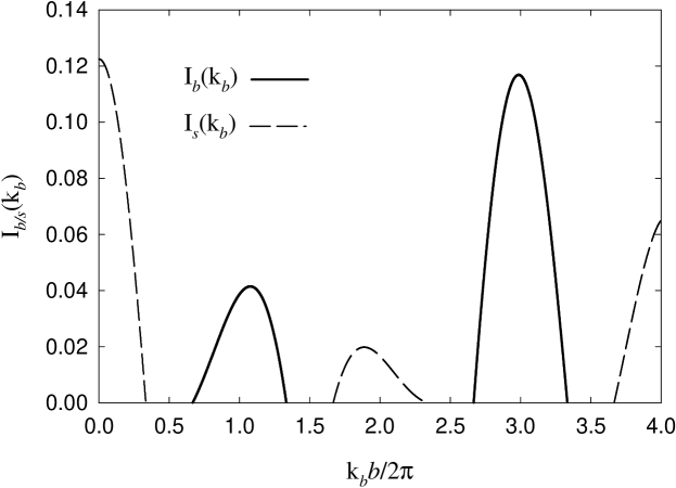
FIG. 2.: Intensity of the bound state mode $I_{b}$, and the intensity of the shadow $I_{s}$ to leading order in the strong coupling expansion. Note that the value of $k_{a}$ is different for the two; in each case it is chosen to maximize the intensity. The intensities are both normalized by the average value of the intensity in the single-particle mode at this order in the strong coupling expansion. The value of $g$ used is $0.7$, which is approximately right for VOPO [2]

The bound state leads to the following basic contribution to the dynamic structure factor for $k_{b}\in(4\pi/3b,8\pi/3b)$ and again for $k_{b}\in(16\pi/3b,20\pi/3b)$:

$$S_{zz}^{\rm bs,basic}({\bf k},\omega) = \frac{g^{2}}{16}(1-4\cos^{2}(\frac{k_{b}b}{4}))\sin^{2}(\frac{k_{b}}{2}(w-\frac{b}{2}))\cos^{2}(\frac{k_{a}v}{2})\delta(\omega-\varepsilon_{B}(k_{b}))\;.$$ (27)

The shadow of the bound state gives for $k_{b}\in(0,2\pi/3b)$, $k_{b}\in(10\pi/3b,14\pi/3b)$ and $k_{b}\in(22\pi/3b,8\pi/b)$:

$$S_{zz}^{\rm bs,shadow}({\bf k},\omega) = \frac{g^{2}}{16}(1-4\sin^{2}(\frac{k_{b}b}{4}))\cos^{2}(\frac{k_{b}}{2}(w-\frac{b}{2}))\sin^{2}(\frac{k_{a}v}{2})\delta(\omega-\varepsilon_{B}^{\rm s}(k_{b}))\;,$$ (28)

where $\varepsilon_{b}^{\rm s}(k_{b})/J=2-g(4\sin^{2}(k_{b}b/4)+1)/4$ gives us the position of the shadow band. The intensity in the bound state mode and in its shadow is depicted are in Fig 2.

We thus see that the bound state mode also acquires a ‘shadow’ as anticipated earlier on the basis of the general argument. Of course, as mentioned previously, this strong-coupling calculation has very little quantitative significance. A quantitative analysis of any experimental data on the bound state mode and it’s shadow would instead follow the analog of the procedure outlined the end of section II with the analog of ${\cal M}_{\sigma}$ included in the analysis and the necessary changes made to allow for the fact that the spectral sum is to be carried out over a different range from the single particle case (note that this type of analysis can, in principle, distinguish between bound state and single particle triplet modes based on the different intensity ratios between the modes and their shadows in the two cases).

IV A more complicated magnetic Hamiltonian?

In this final section we briefly consider a possible complication that will affect our results at a qualitative level: namely the possibility that the magnetic interactions felt by the even and the odd dimers are slightly different. This will clearly change the intensities and the dispersions of the various modes observed as the magnetic Hamiltonian will now be invariant under translations of $b$ and not $b/2$ along the $b$ axis. Thus, the staggering of the dimer positions along the $a$ axis will no longer be the only thing breaking the larger symmetry of translations by $b/2$. Clearly, in such a situation, we expect that the ‘shadow’ band intensity will be non-zero even at $k_{a}=0$ (indeed we expect that it will depend quite sensitively on the difference in the magnetic interactions of the even and odd dimers). To get a feel for what to expect, let us work out the intensity of the basic single particle mode and its shadow to leading order within a strong coupling expansion.

The Hamiltonian we have in mind can be parameterized as:

$${\cal H} = J\sum\limits_{j\,odd}[(1+g\lambda){\bf S}_{I}(j)\cdot{\bf S}_{II}(j)+g(1+\mu){\bf S}_{II}(j)\cdot{\bf S}_{I}(j+1)]$$ (30)

$$+\;J\sum\limits_{j\,even}[(1-g\lambda){\bf S}_{I}(j)\cdot{\bf S}_{II}(j)+g(1-\mu){\bf S}_{II}(j)\cdot{\bf S}_{I}(j+1)]\;,$$

where we have in mind that $\lambda$ and $\mu$ are both small parameters that model the small differences in the magnetic properties of the even and the odd dimers.

The calculation of the ${\cal O}(g)$ single-particle contribution to the dynamic structure factor is quite elementary and involves nothing new. We will therefore be correspondingly brief.

We begin our analysis by noting that it is now more natural to count states somewhat differently. We will restrict the momentum carried by the single particle state to lie in the range $(0,2\pi/b)$ and allow for two distinct bands of single particle states labeled by $+$ and $-$ subscripts.

The energies of these two bands are easily worked out to leading order to be

$$\varepsilon_{\pm}(q)=1\mp\frac{g}{2}(4{\lambda}^{2}+\cos^{2}(qb/2)+{\mu}^{2}\sin^{2}(qb/2))^{1/2}\;.$$ (31)

Moreover, it is quite elementary to see that the corresponding eigenstates to leading order in the strong coupling expansion are (again we choose to write down the state with $S_{z}=0$ as this is what we need to calculate the $zz$ component of the dynamic structure factor):

$$|q_{\pm}[0]\rangle=(\frac{b}{2L})^{1/2}\sqrt{2}{\cal P}(q)(\sum\limits_{j\,odd}e^{iqx^{b}_{j}}|j[0]\rangle+y_{\pm}(q)\sum\limits_{j\,even}e^{iqx^{b}_{j}}|j[0]\rangle)\;,$$ (32)

where ${\cal P}(q)=1/\sqrt{1+|y_{\pm}(q)|^{2}}$ and $y_{\pm}(q)$ is given as

$$y_{\pm}(q)=\frac{2\lambda\pm(4{\lambda}^{2}+\cos^{2}(qb/2)+{\mu}^{2}\sin^{2}(qb/2))^{1/2}}{\cos(qb/2)+i\mu\sin(qb/2)}$$ (33)

One other thing we need is the ground state for this model, correct to ${\cal O}(g)$. This can also be worked out quite easily to be [14]

$$|\Phi_{0}\rangle = |0\rangle+\frac{g(1+\mu)}{8}\sum\limits_{j\,odd}\left(|(j)[0],(j+1)[0]\rangle-|(j)[-1],(j+1)[+1]\rangle-|(j)[+1],(j+1)[-1]\rangle\right)$$ (35)

$$+\;\frac{g(1-\mu)}{8}\sum\limits_{j\,even}\left(|(j)[0],(j+1)[0]\rangle-|(j)[-1],(j+1)[+1]\rangle-|(j)[+1],(j+1)[-1]\rangle\right)$$

We can now use all of this to work out the one particle piece of the dynamic structure factor.

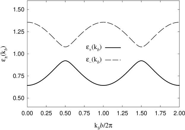
FIG. 3.: Position of the two single particle bands when the interactions felt by the even and odd dimers are different. As explained in the text, the ‘basic mode’ and it’s ‘shadow’ are actually both hybrids made up of the two single particle bands in the problem. We have chosen, for illustrative purposes, the values $\lambda=0.1$ and $\mu=0.1$. The parameter $g$ is set equal to $0.7$, which is approximately correct for VOPO [2].

The resulting expressions are quite messy for general ${\bf k}$ and not particularly illuminating. We will write them down here only for the special case of $k_{a}=0$, as this is where we expect a real qualitative difference due to the complications we have introduced into the problem:

$$S_{zz}({\bf k},\omega) = \sum\limits*12_{\alpha=\pm}\frac{\sin^{2}(k_{b}w/2)}{4}\left[(1+\frac{2G_{\alpha}\cos(k_{b}b/2)}{G^{2}_{\alpha}+Q^{2}})+\frac{g}{2}(\cos(k_{b}b/2)+\frac{2Q^{2}G_{\alpha}}{G^{2}_{\alpha}+Q^{2}})\right]$$ (38)

$$~{}~{}~{}~{}~{}~{}~{}~{}~{}~{}~{}~{}~{}~{}~{}~{}~{}~{}~{}~{}~{}~{}\times\;\delta(\omega-\varepsilon_{\alpha}(k_{b}))\;,$$

where we have defined $Q^{2}$ as

$$Q^{2}(k_{b})=\cos^{2}(k_{b}b/2)+\mu^{2}\sin^{2}(k_{b}b/2)\;,$$ (39)

and $G$ as

$$G_{\pm}(k_{b})=2\lambda\pm\sqrt{4\lambda^{2}+Q^{2}(k_{b})}\;.$$ (40)

The details of the above expressions are not particularly important. We only wish to use the above to arrive at some general qualitative conclusions about the nature of the expected intensity at various points in the Brillouin zone. The first of these is of course that we have some non-zero intensity at the shadow positions even at $k_{a}=0$. In this context, it is important to note that both the ‘basic mode’ and the ‘shadow’ are actually hybrids made up of the $+$ band and the $-$ band. For small enough $\mu$ and $\lambda$, the intensity switches between the two in such a manner that we have one approximately continuous basic mode and another much weaker shadow mode that is also approximately continuous.

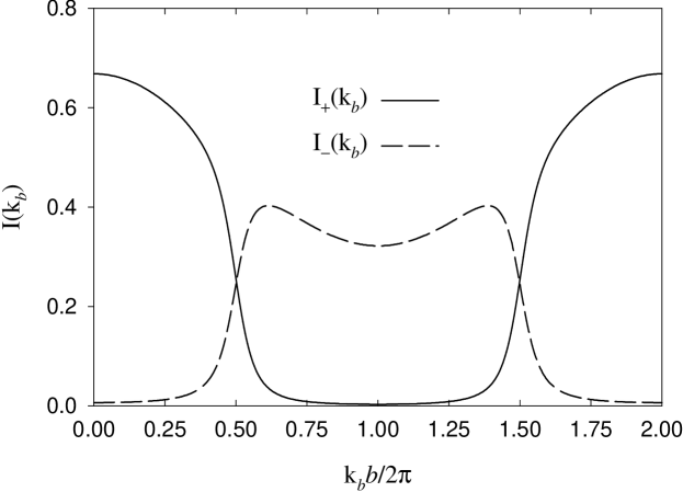
FIG. 4.: Intensity at $k_{a}=0$ of the two single particle bands when the interactions felt by the even and odd dimers are different. For clarity, the $\sin^{2}(k_{b}w/2)$ modulation of the intensity is not included in the plots. The values of $\lambda$, $\mu$ and $g$ are set as in Fig 3.

These results are summarized in Fig 3 and Fig 4. Of course, the avoided level crossing between the two bands leads to a small jump in position of both the basic and the shadow mode situated near $\pi/b$ and $3\pi/b$. Thus the intensity at the shadow positions and the gap introduced by the avoided level crossing are sensitive indicators of the difference between the magnetic environments of even and odd dimers. As mentioned earlier, all experiments to date [2, 6, 8] are consistent with the absence of extra modes at $k_{a}=0$, but in the absence of any straightforward symmetry reason, more experiments at $k_{a}=0$ with better sensitivity and statistics are necessary before one can completely rule out the existence of such complications in the magnetic Hamiltonian of the system.

V Conclusion

The calculations presented here show that simple geometric effects can lead to the presence of the shadow bands observed recently in VOPO. These modes are similar to the ‘optic’ modes that can arise generally in coupled alternating-chain systems with more than one dimer per unit cell, for example the ‘chain’ layers in Sr₁₄Cu₂₄O₄₁ [15]. However, in VOPO the shadow modes arise from a single chain. It should be possible to test our proposal by comparing the experimentally observed intensity ratios with our predictions. Moreover, as mentioned earlier, the intensity ratios can also distinguish between single-particle and bound state modes The possible contribution of the triplet bound state to the spin dynamics in VOPO remains an open question at this time.

VI Acknowledgements

KD would like to thank the Neutron Scattering Group at ORNL for hospitality, and ORISE for financial support for a visit during which this work was begun. We thank T. Barnes, M. Enderle, B.C. Sales, H. Schwenk and D.A. Tennant for numerous helpful discussions. Work at Princeton was supported by NSF grant DMR-9809483. The Oak Ridge National Laboratory is managed for the U.S. D.O.E. by Lockheed Martin Energy Research Corporation under contract DE-AC05-96OR22464.

REFERENCES

- [1] R.S. Eccleston et al., Phys. Rev. Lett. 73, 2626 (1994) and references therein.
- [2] A. W. Garrett et al., Phys. Rev. Lett. 79, 745 (1997).
- [3] G.S. Uhrig and H.J. Schulz, Phys. Rev. B 54, R9624 (1996).
- [4] G.S. Uhrig and B. Normand, Phys. Rev. B 58, R14705 (1998); see also A. Weisse, G. Bouzerar, and H. Fehske, Eur. Phys. J. B. 7, 5 (1999).
- [5] J. Kikuchi et al., cond-mat/9902205.
- [6] M. Enderle et al., Bull. Am. Phys. Soc. 44, 1884 (1999), to be published.
- [7] T. Barnes, J. Riera, and D. A. Tennant, cond-mat/9801224.
- [8] A. W. Garrett, Ph.D thesis, University of Florida (1997), unpublished.
- [9] P.T. Nguyen et al., Mater. Res. Bull. 30, 1055 (1995).
- [10] B. Leuenberger et al., Phys. Rev. B 30, 6300 (1984).
- [11] S. Sachdev and R. Bhatt, Phys. Rev. B 41, 9323 (1990).
- [12] R.A. Cowley, B. Lake and D.A. Tennant, J. Phys. Cond. Matt. 8, L179, (1996).
- [13] K. Damle and S. Sachdev, Phys. Rev. B 57, 8307 (1998).
- [14] K. Damle, unpublished.
- [15] M. Matsuda et al., Phys. Rev. B 59, 1060 (1999).