First- principle calculations of magnetic interactions in correlated systems

Abstract

We present a novel approach to calculate the effective exchange interaction parameters based on the realistic electronic structure of correlated magnetic crystals in local approach with the frequency dependent self energy. The analog of “local force theorem” in the density functional theory is proven for highly correlated systems. The expressions for effective exchange parameters, Dzialoshinskii- Moriya interaction, and magnetic anisotropy are derived. The first-principle calculations of magnetic excitation spectrum for ferromagnetic iron, with the local correlation effects from the numerically exact QMC-scheme is presented.

I Introduction

The calculation of thermodynamic properties and excitation spectra of different magnetic materials is one of the most important motivations of the microscopic theory of magnetism. The main approach for such type of investigations is the local spin density functional (LSDF) scheme [1]. However, this method has some serious shortcomings when applying to transition metal and rare-earth magnetic materials. The main defect is the absence of the “Hubbard” type correlations which are most important for real magnets (see, e.g., recent reviews [2, 3, 4]). This leads to, generally speaking, incorrect description of electronic structure for such important groups of magnetic materials as rare-earth metals and their compounds, metal-oxide compounds (including “classical” Mott insulators such as NiO and MnO as well as high-$T_{c}$ cuprates) and even for the iron-group metals [2, 4, 5]. At the same time, the experience with the Hubbard model shows that the description of electronic structure and magnetic properties of highly correlated materials are closely connected. Recently we propose a rather general scheme (so-called “LDA++ approach”) for first-principle calculations of the electronic structure with the local correlation effects being included [5]. In this technique the full matrix of on-site Coulomb repulsion for the correlated states is taken into account in the local approximation for the electron self- energy. In such a way, we could provide a rather reasonable description of the electronic structure for different correlated systems such as Fe, NiO, and TmSe. It will be very useful to develop this approach for the description of different magnetic characteristics.

The most rigorous way to consider properties of magnetic excitations is the calculation of frequency-dependent magnetic susceptibilities[4]. However, for many important cases we can restrict ourselves to more simple problem of the calculation of static response functions. More explicitly, one can consider the variations of total energy $E_{tot}$ (or thermodynamic potential $\Omega$) with respect to magnetic moments rotations. This approach results in the magnetic interactions of different types: the variation of total energy of a ferromagnet over the rotation of all spins at the same angle determines the magnetic anisotropy energy, while the variation of $E_{tot}$ over the relative rotations of spins on two sites gives the parameters of pairwise exchange interactions, etc. This approach was proposed earlier in the the framework of the LSDF scheme [7]. It is sufficient for the calculation of “phenomenological” exchange parameters which are important for the consideration of domain wall widths and other “micromagnetic” properties. In the adiabatic approximation when the energies of magnetic excitations are small in comparison with typical electronic energies this is also sufficient for the calculation of the spin-wave spectrum. In the mean-field approximation these “exchange parameters” can be used for the estimation of Curie or Neel temperature.

In this work we derive general expressions for the parameters of magnetic interactions in LDA++ approach and calculate the exchange parameters for ferromagnetic iron. It is a first attempt to investigate magnetic interactions, taking into account correlation effects in the electronic structure for real materials.

II General formalism

A Local force theorem in LDA++ approach

An important trick for the definition of exchange interactions in the LSDF approach is the use of so called ”local force theorem”. This reduces the calculation of the total energy change to the variations of one-particle density of states [6, 7]. First of all, let us prove the analog of local force theorem in the LDA++ approach. In contrast with the standard density functional theory, it deals with the real dynamical quasiparticles defined via Green functions for the correlated electrons rather than with Kohn-Sham “quasiparticles” which are, strictly speaking, only auxiliary states to calculate the total energy. Therefore, instead of the working with the thermodynamic potential $\Omega$ as a density functional we have to start from its general expression in terms of an exact Green function [8]

$$\Omega = \Omega_{sp}-\Omega_{dc}$$ (1)

$$\Omega_{sp} = -Tr\left\{\ln\left[\Sigma-G_{0}^{-1}\right]\right\}$$ (2)

$$\Omega_{dc} = Tr\Sigma G-\Phi$$ (3)

where $G,G_{0}$ and $\Sigma$ are an exact Green function, its bare value and self-energy, correspondingly; $\Phi$ is the Luttinger generating functional (sum of the all connected skeleton diagrams without free legs), $Tr=Tr_{\omega iL\sigma}$ is the sum over Matsubara frequencies $Tr_{\omega}...=T\sum\limits_{\omega}...,$ $\omega=\pi T\left(2n+1\right),$ $n=0,\pm 1,...,$ $T$ is the temperature, and $iL\sigma$ are site numbers ($i$), orbital quantum numbers ($L={l,m}$) and spin projections $\sigma$ , correspondingly. We have to keep in mind also Dyson equation

$$G^{-1}=G_{0}^{-1}-\Sigma$$ (4)

and the variational identity

$$\delta\Phi=Tr\Sigma\delta G.$$ (5)

We represent the expression (1) as a difference of ”single particle” ($sp$) and ”double counted” ($dc$) terms as it is usual in the density functional theory. When neglecting the quasiparticle damping, $\Omega_{sp}$ will be nothing but the thermodynamic potential of ”free” fermions but with exact quasiparticle energies. Suppose we change the external potential, for example, by small spin rotations. Then the variation of the thermodynamic potential can be written as

$$\delta\Omega=\delta^{*}\Omega_{sp}+\delta_{1}\Omega_{sp}-\delta\Omega_{dc}$$ (6)

where $\delta^{*}$ is the variation without taking into account the change of the ”self-consistent potential” (i.e. self energy) and $\delta_{1}$ is the variation due to this change of $\Sigma$. Taking into account Eq. (5) it can be easily shown (cf. [8]) that

$$\delta_{1}\Omega_{sp}=\delta\Omega_{dc}=TrG\delta\Sigma$$ (7)

and hence

$$\delta\Omega=\delta^{*}\Omega_{sp}=-\delta^{*}Tr\ln\left[\Sigma-G_{0}^{-1}\right]$$ (8)

which is an analog of the ”local force theorem” in the density functional theory [7]. In the LSDF scheme all the computational results expressed in terms of the retarded Green function and not in the Matsubara one. The relations of “real” and “complex” Green-function formulae are based on the identity

$$Tr_{\omega}F(i\omega)=-\frac{1}{\pi}\int\limits_{-\infty}^{\infty}dzf(z)ImF(z+i0)$$ (9)

where $f(z)=\left[\exp z/T+1\right]^{-1}$ is the Fermi function, $F(z)$ is a function regular in all the complex plane except real axis. Therefore Eq.(8) takes the following form

$$\delta\Omega=\frac{1}{\pi}\int\limits_{-\infty}^{\infty}dzf(z)ImTr_{iL\sigma}\ln G^{-1}(z+i0)$$ (10)

which is the starting point for the calculations of magnetic interactions in LSDF approach [7]. However note, that in the case of frequency-dependent self-energy (LDA++ approach) it is more convenient to work with the Matsubara Green functions [5].

B Effective spin Hamiltonian

Further considerations are similar to the corresponding ones in LSDF approach. The most suitable way based on the sum rule is proposed in [9].

In the LDA++ scheme, the self energy is local, i.e. is diagonal in site indices. Let us write the spin-matrix structure of the self energy and Green function in the following form

$$\Sigma_{i} = \Sigma_{i}^{c}+{\bf\Sigma}_{i}^{s}{\bf{\sigma}}$$ (11)

$$G_{ij} = G_{ij}^{c}+{\bf G}_{ij}^{s}{\bf{\sigma}}$$ (12)

where $\Sigma_{i}^{\left(c,s\right)}=\frac{1}{2}\left(\Sigma_{i}^{\uparrow}\pm\Sigma_{i}^{\downarrow}\right)$, ${\bf\Sigma}_{i}^{s}=\Sigma_{i}^{s}{\bf e}_{i},$ with ${\bf e}_{i}$ being the unit vector in the direction of effective spin-dependent potential on site $i$, ${\bf{\sigma}}=(\sigma_{x},\sigma_{y},\sigma_{z})$ are Pauli matrices, $G_{ij}^{c}=\frac{1}{2}Tr_{\sigma}(G_{ij})$ and ${\bf G}_{ij}^{s}=\frac{1}{2}Tr_{\sigma}(G_{ij}{\bf{\sigma}})$. We assume that the bare Green function $G^{0}$ does not depend on spin directions and all the spin-dependent terms including the Hartree-Fock terms are incorporated in the self energy. Spin excitations with low energies are connected with the rotations of vectors ${\bf e}_{i}$:

$$\delta{\bf e}_{i}=\delta{\bf\varphi}_{i}\times{\bf e}_{i}$$ (13)

According to the ”local force theorem” (8) the corresponding variation of the thermodynamic potential can be written as

$$\delta\Omega=\delta^{*}\Omega_{sp}={\bf V}_{i}\delta{\bf\varphi}_{i}$$ (14)

where the torque is equal to

$${\bf V}_{i}=2Tr_{\omega L}\left[{\bf\Sigma}_{i}^{s}\times{\bf G}_{ii}^{s}\right]$$ (15)

Further we have to use an important sum rule for the Green function which is the consequence of Dyson equation. Using Eq.(4) one has

$$G = G^{c}\cdot\widehat{I}+{\bf G}^{s}\cdot{\bf{\sigma}}=GG^{-1}G=$$ (17)

$$\ \ G\left(\left(G_{0}^{-1}-\Sigma^{c}\right)\cdot\widehat{I}-{\bf\Sigma}^{s}\cdot{\bf{\sigma}}\right)\left(G^{c}\cdot\widehat{I}+{\bf G}^{s}\cdot{\bf{\sigma}}\right).$$

Separating the spin-dependent and the spin-independent parts in Eq. (17) we have the following sum rules for $G^{c}$

$$G^{c}=G^{c}\left(G_{0}^{-1}-\Sigma^{c}\right)G^{c}-G^{c}{\bf\Sigma}^{s}{\bf G}^{s}=G^{c}\left(G_{0}^{-1}-\Sigma^{c}\right)G^{c}-{\bf G}^{s}{\bf\Sigma}^{s}G^{c}$$ (18)

and similarly for ${\bf G}^{s}$

$${\bf G}^{s} = -\left({\bf G}^{s}{\bf\Sigma}^{s}\right){\bf G}^{s}+G^{c}{\bf\Sigma}^{s}G^{c}+iG^{c}\left({\bf\Sigma}^{s}\times{\bf G}^{s}\right)=$$ (19)

$$= -{\bf G}^{s}\left({\bf\Sigma}^{s}{\bf G}^{s}\right)+G^{c}{\bf\Sigma}^{s}G^{c}+i\left({\bf G}^{s}\times{{\bf\Sigma}}^{s}\right)G^{c}$$ (20)

Then for diagonal elements of the Green function one obtains

$${\bf G}_{ii}^{s}=-\sum_{j}\left[\left({\bf G}_{ij}^{s}{\bf\Sigma}_{j}^{s}\right){\bf G}_{ji}^{s}-G_{ij}^{c}{\bf\Sigma}_{j}^{s}G_{ji}^{c}-iG_{ij}^{c}\left({\bf\Sigma}_{j}^{s}\times{\bf G}_{ji}^{s}\right)\right]$$ (21)

Substituting (21) into (15) we have the following expression for the torque

$${\bf V}_{i} = 2Tr_{\omega L}\left[{\bf\Sigma}_{i}^{s}\times{\bf G}_{ii}\right]$$ (22)

$$= -2\sum_{j}Tr_{\omega L}\left\{{\bf\Sigma}_{i}^{s}\times\left({\bf G}_{ij}^{s}{\bf\Sigma}_{j}^{s}\right){\bf G}_{ji}^{s}-{\bf\Sigma}_{i}^{s}\times G_{ji}^{c}{\bf\Sigma}_{j}^{s}G_{ij}^{c}-i{\bf\Sigma}_{i}^{s}\times G_{ji}^{c}\left({\bf\Sigma}_{j}^{s}\times{\bf G}_{ji}^{s}\right)\right\}$$ (23)

If we represent the total thermodynamic potential of spin rotations or the effective Hamiltonian in the form

$$\Omega_{spin}=-\sum_{ij}Tr_{\omega L}\left\{\left({\bf G}_{ij}^{s}{\bf\Sigma}_{j}^{s}\right)\left({\bf G}_{ji}^{s}{\bf\Sigma}_{i}^{s}\right)-{\bf\Sigma}_{i}^{s}G_{ij}^{c}{\bf\Sigma}_{j}^{s}G_{ji}^{c}-i\left({\bf\Sigma}_{i}^{s}\times G_{ij}^{c}{\bf\Sigma}_{j}^{s}\right){\bf G}_{ji}^{s}\right\}$$ (24)

one can show by direct calculations that

$$\left[\frac{\delta\Omega_{spin}}{\delta{\bf\varphi}_{i}}\right]_{G=const}={\bf V}_{i}$$ (25)

This means that $\Omega_{spin}\left\{{\bf e}_{i}\right\}$ is the effective spin Hamiltonian. The last term in Eq.(24) is nothing but Dzialoshinskii- Moriya interaction term. It is non-zero only in relativistic case where ${\bf\Sigma}_{j}^{s}$ and ${\bf G}_{ji}^{s}$ can be, generally speaking, “non-parallel” and $G_{ij}\neq G_{ji}$ for the crystals without inversion center. In the following we will not consider this term.

C Exchange interactions

In the nonrelativistic case one can rewrite the spin Hamiltonian for small spin deviations near collinear magnetic structures in the following form

$$\Omega_{spin}=-\sum_{ij}J_{ij}{\bf e}_{i}{\bf e}_{j}$$ (26)

where

$$J_{ij}=-Tr_{\omega L}\left(\Sigma_{i}^{s}G_{ij}^{\uparrow}\Sigma_{j}^{s}G_{ji}^{\downarrow}\right)$$ (27)

are the effective exchange parameters. This formula generalize the LSDA expressions of [7] to the case of correlated systems.

The sum rule (Eq. 21) for the collinear magnetic configuration takes the following form

$$G_{ii}^{\uparrow}-G_{ii}^{\downarrow}=2\sum\limits_{j}G_{ij}^{\uparrow}\Sigma_{j}^{s}G_{ji}^{\downarrow}$$ (28)

Using Eq. (28) we obtain the following expression for the total exchange interaction of a given site with the all magnetic environment.

$$J_{i}=\sum\limits_{j(\neq i)}J_{ij}=Tr_{\omega L}\left[\Sigma_{i}^{s}G_{ii}^{\uparrow}\Sigma_{i}^{s}G_{ii}^{\downarrow}-\frac{1}{2}\Sigma_{i}^{s}\left(G_{ii}^{\uparrow}-G_{ii}^{\downarrow}\right)\right]$$ (29)

Spin wave spectrum in ferromagnets can be considered both directly from the exchange parameters or by the consideration of the energy of corresponding spiral structure (cf [7]). In nonrelativistic case when the anisotropy is absent one has

$$\omega_{{\bf q}}=\frac{4}{M}\sum\limits_{j}J_{0j}\left(1-\cos{\bf qR}_{j}\right)\equiv\frac{4}{M}[J(0)-J({\bf q})]$$ (30)

where $M$ is the magnetic moment (in Bohr magnetons) per magnetic ion. Corresponding expressions can be easily written in k-space also. In the short notation $q=({\bf q},i\omega)$ it is easy to write the general expression for $J({{\bf q)}\equiv}J({\bf q},0)$:

$$J(q)=-\frac{1}{N_{k}}\sum_{k}Tr_{L}[\Sigma^{s}(k)G^{\uparrow}(k)\Sigma^{s}(k+q)G^{\downarrow}(k+q)]$$ (31)

where $N_{k}$ is the total number of k-points.

It should be noted that the expression for spin stiffness tensor $D_{\alpha\beta}$ defined by the relation

$$\omega_{{\bf q}}=D_{\alpha\beta}q_{\alpha}q_{\beta}$$ (32)

(${\bf q\rightarrow 0}$) in terms of exchange parameters has to be exact since it is the consequence of phenomenological Landau- Lifshitz equations which are definitely correct in the long-wavelength limit (cf [7]). One has from Eqs. (27,30)

$$D_{\alpha\beta}=\frac{2}{M}\sum\limits_{j}J_{0j}R_{j}^{\alpha}R_{j}^{\beta}=-\frac{2}{M}Tr_{\omega L}\sum\limits_{{\bf k}}\left(\Sigma^{s}\frac{\partial G^{\uparrow}\left({\bf k}\right)}{\partial k\alpha}\Sigma^{s}\frac{\partial G^{\downarrow}\left({\bf k}\right)}{\partial k_{\beta}}\right)$$ (33)

where ${\bf k}$ is the quasimomentum and the summation is over the Brillouin zone. In cubic crystals $D_{\alpha\beta}=D\delta_{\alpha\beta}$. For arbitrary ${\bf q}$, the expression of magnon spectrum in terms of $J_{ij}$ is valid only in the adiabatic approximation, i.e. provided that the magnon frequencies are small in comparison with characteristic electronic energies. Otherwise, collective magnetic excitations which are magnons cannot be separated from non-coherent particle-hole excitations (Stoner continuum) [10] and magnon frequencies (30) are not the exact poles of transverse magnetic susceptibility (which are even not real at large ${\bf q}$).

Now we have to consider the accuracy of expressions for $J_{ij}$ (27) themselves. Eqs. (15) and (22) are exact in LDA++ approach (i.e. with the only assumption about the local self-energy). Hence, if one postulate the existence of effective spin Hamiltonian in the sense of Eq.(25), Eq. (27) is also exact. However, they do not have rigorous connection with the static transverse spin susceptibility. The latter is expressed in terms of the matrix

$\displaystyle\frac{\delta^{2}\Omega}{\delta\varphi_{i}^{\alpha}\delta\varphi_{j}^{\beta}}=\frac{\delta V_{i}^{\alpha}}{\delta\varphi_{j}^{\beta}}$

without the restriction $G=const.$ They differ from our exchange parameters by the terms containing $\frac{\delta\widehat{G}}{\delta{\bf\varphi}_{i}}.$ From the diagrammatic point of view in the framework of DMFT [4] they are nothing but the vertex corrections. We do not present the corresponding expressions since the benefits of the introducing of exchange parameters beyond adiabatic approximation which is equivalent to (25) is doubtful. In more rigorous consideration it is convenient to work directly with DMFT expressions for static and dynamic susceptibility [4].

Thus one can see that, generally speaking,the exchange parameters differ from the exact response characteristics defined via static susceptibility since the latter contains vertex corrections. At the same time, our derivation of exchange parameters seems to be rigorous in the adiabatic approximation for spin dynamics when spin fluctuation frequency is much smaller than characteristic electron energy. The situation is similar to the case of electron-phonon interactions where according to the Migdal theorem vertex corrections are small in adiabatic parameter (ratio of characteristic phonon energy to electron one)[12]. The derivation of the exchange parameters from the variations of thermodynamic potential, being approximate, can be useful nevertheless for the fast and accurate calculations of different magnetic systems.

Note that in the LDA++ approach, as well as in LDA+U method and in contrast with usual LSDF, one can rotate separately spins of states with given orbital quantum numbers $L,L^{\prime}$ . For example, for non-relativistic case one can obtain

$\displaystyle\Omega_{spin}=-\sum_{iL,jL^{\prime}}J_{iL,jL^{\prime}}{\bf e}_{iL}{\bf e}_{jL^{\prime}}$

where

$\displaystyle J_{iL,jL^{\prime}}=-Tr_{\omega}\left(\Sigma_{iL}^{s}G_{iL,jL^{\prime}}^{\uparrow}\Sigma_{jL^{\prime}}^{s}G_{jL^{\prime},iL}^{\downarrow}\right)$

are orbital dependent exchange parameters.

D Magnetic anisotropy

Let us consider now the change of spin energy at the rotation of all the spins at the same angle. It is definitely zero in nonrelativistic case. In the presence of spin-orbit coupling, it is nothing but the energy of magnetic anisotropy. One can obtain from Eq.(24)

$$\Omega_{anis} = Tr_{\omega L}\sum\limits_{ij}\left\{\left({\bf G}_{ij}^{s}\times{\bf\Sigma}_{j}^{s}\right)\left({\bf G}_{ji}^{s}\times{\bf\Sigma}_{i}^{s}\right)\right\}=$$ (35)

$$\ \ Tr_{\omega L}\sum\limits_{{\bf k}}\left\{\left({\bf G}^{s}\left({\bf k}\right)\times{\bf\Sigma}^{s}\right)\left({\bf G}^{s}\left({\bf-k}\right)\times{\bf\Sigma}^{s}\right)\right\}$$

where the last equality is valid for ferromagnets with one magnetic atom per unit cell, k is the quasimomentum and the summation is over Brillouin zone.

Finally, note that we use essentially three properties of LDA++ approach: (i) locality of self-energy (ii) spin-independence of bare Green function (i.e. spin-independence of bare LDA spectrum; all magnetic effects including Hartree-Fock ones are included in self- energy) and (iii) approximations for self energy have to be conserving, or “$\Phi$- derivable” since only in that case analog of “local force theorem” (8) takes place.

III Exchange interactions in ferromagnetic iron

A Computational technique

As an example we calculate the magnetic properties of ferromagnetic iron using the most accurate method to take into account local correlations. For this purpose we use the local quantum Monte-Carlo approach[4] with the generalization to the multiband case[13].

We start from LDA+U Hamiltonian in the diagonal density approximation:

$$H = \sum_{\{im\sigma\}}t_{im,i^{\prime}m^{\prime}}^{LDA}c_{im\sigma}^{+}c_{i^{\prime}m^{\prime}\sigma}+$$ (38)

$$\frac{1}{2}\sum_{imm^{\prime}\sigma}U_{mm^{\prime}}^{i}n_{im\sigma}n_{im^{\prime}-\sigma}+$$

$$\frac{1}{2}\sum_{im\neq m^{\prime}\sigma}(U_{mm^{\prime}}^{i}-J_{mm^{\prime}}^{i})n_{im\sigma}n_{im^{\prime}\sigma}$$

where $t^{LDA}$ is effective single-particle Hamiltonian obtained from the non-magnetic LDA with the corrections for double counting of the average interactions among d-electrons; $i$ is the site index and $m$ is the orbital quantum numbers; $\sigma=\uparrow,\downarrow$ is the spin projection; $c^{+},c$ are the Fermi creation and annihilation operators ($n=c^{+}c$).

The screened Coulomb and exchange vertex for the d-electrons

$$U_{mm^{\prime}} = <mm^{\prime}|V_{scr}^{ee}({\bf r-r}^{\prime})|mm^{\prime}>$$ (39)

$$J_{mm^{\prime}} = <mm^{\prime}|V_{scr}^{ee}({\bf r-r}^{\prime})|m^{\prime}m>$$ (40)

are expressed via the effective Slater integrals and corresponds to the average $U=2.3$ eV and $J=0.9$ eV[5]. We use the minimal $spd$-basis in the LMTO-TB formalism and numerical orthogonalization for $t^{LDA}({\bf k})$ matrix [5]. The Matsubara frequencies summation in our calculations corresponds to the temperature of about T=850 K.

Local Green-function matrix has the following form

$$G(i\omega)=\sum_{{\bf k}}\{i\omega+\mu-t^{LDA}({\bf k})-\Sigma(i\omega)\}^{-1}$$ (41)

Note that due to cubic crystal symmetry of ferromagnetic bcc-iron the local Green function is diagonal both in the orbital and the spin indices and the bath Green function is defined as

$$G_{m}^{0}(i\omega)=G_{m}(i\omega)+\Sigma_{m}(i\omega)$$ (42)

The local Green functions for the imaginary time interval $\left[0,\beta\right]$ with the mesh $\tau_{l}=l\Delta\tau$, $l=0,...,L-1,$ and $\Delta\tau=\beta/L$, where $\beta=\frac{1}{T}$ is calculated in the path-integral formalism[4, 13]:

$$G_{m}^{ll^{\prime}}=\frac{1}{Z}\sum_{s_{mm^{\prime}}^{l}}\det[O(s)]*G_{m}^{ll^{\prime}}(s)$$ (43)

here we redefined for simplicity $m\equiv\{m,\sigma\},Z$ is the partition function and the so-called fermion-determinant $\det[O(s)]$ and the Green function for arbitrary set of the auxiliary fields $G(s)=O^{-1}(s)$ are obtained via the Dyson equation[14] for imaginary-time matrix $({\bf G}_{m}(s)\equiv G_{m}^{ll^{\prime}}(s))$:

$\displaystyle{\bf G}_{m}=[{\bf 1}-({\bf G}_{m}^{0}-{\bf 1})(e^{V_{m}}-{\bf 1})]^{-1}{\bf G}_{m}^{0}$

where the effective fluctuation potential from the Ising fields $s_{mm^{\prime}}^{l}=\pm 1$ is

$$V_{m}^{l} = \sum_{m^{\prime}(\neq m)}\lambda_{mm^{\prime}}s_{mm^{\prime}}^{l}\sigma_{mm^{\prime}}$$

$$\sigma_{mm^{\prime}} = \{\begin{array}[]{c}1,m<m^{\prime}\\ -1,m>m^{\prime}\end{array}$$

and the discrete Hubbard-Stratonovich parameters are $\lambda_{mm^{\prime}}={\rm arccosh}[\exp(\frac{1}{2}\Delta\tau U_{mm^{\prime}})]$ [14]. The main problem of the multiband QMC formalism is the large number of the auxiliary fields $s_{mm^{\prime}}^{l}.$ For each time slices $l$ it is equals to $M(2M-1)$ where$M$ is the total number of the orbitals which is equal to 45 for d-states. We compute the sum over this auxiliary fields in Eq.43 using important sampling QMC algorithm and performed a dozen of self-consistent iterations over the self-energy Eqs.(41,42,43). The number of QMC sweeps was of the order of 10⁵ on the CRAY-T3e. The final $G_{m}(\tau)$ has very little statistical noise. We use maximum entropy method[15] for analytical continuations of the QMC Green functions to the real axis. Comparison of the total density of states with the results of LSDA calculations (Fig.1) shows a reasonable agreement for single-particle properties of not “highly correlated” ferromagnetic iron.

Using the self-consistent values for $\Sigma_{m}(i\omega)$ we calculate the exchange interactions (Eq.31) and spin-wave spectrum (Eq.30) using the four-dimensional fast Fourier transform (FFT) method[11] for $({\bf k},i\omega)$ space with the mesh $20^{3}\times 320$. We compare the results for the exchange interactions with corresponding calculations for the LSDA method[7].

B Computational results

The spin-wave spectrum for ferromagnetic iron is presented in Fig.2 in comparison with the results of LSDA-exchange calculations and with different experimental data[16, 17, 18] . Note that for high-energy spin-waves the experimental data[18] has large error-bars due to Stoner damping (we show one experimental point with the uncertainties in the “$q$” space). On the other hand, the expression of magnon frequency in terms of exchange parameters itself becomes problematic in that region due to breakdown of adiabatic approximation, as it is discussed above. Therefore we do not believe that good agreement of LSDA data with the experimental ones for large wave vectors is too important since it may be a result of ”mutual cancellation” of inaccuracies of adiabatic approximation and LSDA itself. At the same time, our lower-energy spin-waves spectrum (where the theory is reliable) agree better with the experiments then the result of LSDA calculations. Our LSDA spin-wave spectrum agree well with the results of frozen magnon calculations [19, 20]. Note that in the LSDA scheme one could use the linear-response formalism[21] to calculate the spin-wave spectrum with the Stoner renormalizations, which should gives in principle the same spin-wave stiffness as our LSDA calculations. The corresponding exchange parameters and spin-waves stiffness (Eq.32) are presented in the Table I. The general trend in the distance dependence of exchange interactions in ferromagnetic iron is similar in both schemes, but relative strength of various interactions is quite different. Experimental value of spin-wave stiffness D=280 meV/A²[17] agrees well with the theoretical LDA++ estimations.

IV Conclusions

In conclusion, we present a general method for the investigation of magnetic interactions in the correlated electron systems. This scheme is not based on the perturbation theory in “$U$” and could be applied for rare-earth systems where both the effect of the band structure and the multiplet effects are crucial for a rich magnetic phase diagram. Our general expressions are valid in relativistic case and can be used for the calculation of both exchange and Dzialoshinskii- Moriya interactions, and magnetic anisotropy. An illustrative example of ferromagnetic iron shows that the correlation effects in exchange interactions may be noticeable even in such moderately correlated systems. For rare-earth metals and their compounds, colossal magnetoresistance materials or high-$T_{c}$ systems, this effect may be much more important. For example, the careful investigations of exchange interactions in $MnO$ within the LSDA, LDA+U and optimized potential methods for $MnO$ [22] show the disagreement with experimental spin-wave spectrum (even for small ${\bf q}$) , and indicate a possible role of correlation effects.

As for the formalism itself, this work demonstrates an essential difference between spin density functional approach and LDA++ method. The latter deals with the thermodynamic potential as a functional of Green function rather than electron density. Nevertheless, there is a deep formal correspondence between two techniques (self-energy corresponds to the exchange- correlation potential, etc). In particular, an analog of local force theorem can be proved for LDA++ approach. It may be useful not only for the calculation of magnetic interactions but also for elastic stresses, in particular, pressure, and other physical properties.

V Acknowledgments

The calculations were performed on Cray T3E computers in the Forschungszentrum Jülich with grants of CPU time from the Forschungszentrum and John von Neumann Institute for Computing (NIC). This work was partially supported by Russian Basic Research Foundation, grant 98-02-16279

TABLE I.: Parameters of exchange interactions and spin-wave stiffness for ferromagnetic iron calculated with the LSDA and LDA+$\Sigma$ methods.

meV	J0	J1	J2	J3	J4	J5	J6	D (meV/A2)
LSDA	166.1	16.48	8.07	0.25	-1.03	-0.31	0.26	320
LDA+$\Sigma$	115.8	13.31	2.5	0.73	-0.38	-0.83	0.01	260

 

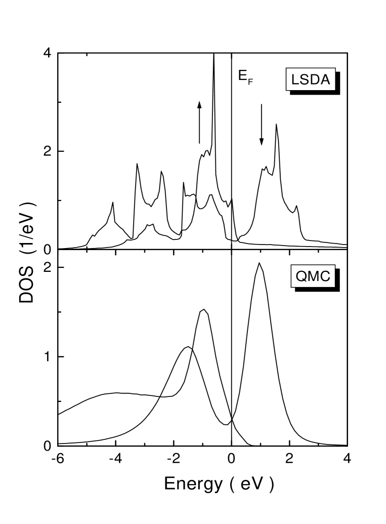
FIG. 1.: Total spin-polarized density of states for ferromagnetic iron in the LSDA and LDA+QMC approximations.

 

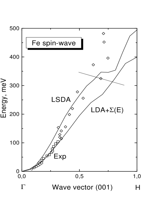
FIG. 2.: The spin-wave spectrum for ferromagnetic iron in the LSDA and LDA+$\Sigma$ approximations compared with different experiments (circles [16], squares [17], and diamonds [18]) (a); The corresponding spin-wave spectrum from LDA+$\Sigma$ scheme in the (110) plane (b).

REFERENCES

- [1] R. O. Jones and O. Gunnarsson, Rev. Mod. Phys. 61, 689 (1989).
- [2] P. W. Anderson, 50 Years of the Mott Phenomenon, in: Frontiers and Borderlines in Many Particle Physics, ed. by J. R. Schrieffer and R. A. Broglia (North- Holland, Amsterdam, 1988);
- [3] S. V. Vonsovsky, M. I. Katsnelson, and A. V. Trefilov, Phys. Metals Metallogr. 76, 247, 343 (1993).
- [4] A. Georges, G. Kotliar, W. Krauth, and M. Rozenberg, Rev. Mod. Phys. 68, 13 (1996).
- [5] A. I. Lichtenstein and M. I. Katsnelson, Phys. Rev. B57, 6884 (1998); M. I. Katsnelson and A. I. Lichtenstein, J. Phys.: Cond. Matter 11, 1037 (1999).
- [6] A. R. Mackintosh, O. K. Andersen, In: Electron at the Fermi Surface, ed.M. Springford (Univ. Press, Cambridge, 1980) p.145.
- [7] A. I. Liechtenstein, M. I. Katsnelson, and V. A. Gubanov, J. Phys. F 14, L125; Solid State Commun. 54, 327 (1985); A. I. Liechtenstein, M. I. Katsnelson, V. P. Antropov, and V. A. Gubanov, J. Magn. Magn. Mater. 67, 65 (1987).
- [8] J. M. Luttinger and J. C. Ward, Phys. Rev. 118, 1417 (1960); see also G. M. Carneiro and C. J. Pethick, Phys. Rev. B 11, 1106 (1975).
- [9] V. P. Antropov, M. I. Katsnelson, and A. I. Liechtenstein, Physica B 237-238, 336 (1997).
- [10] T. Moriya, Spin Fluctuations in Itinerant Electron Magnetism (Springer-Verlag, Berlin, 1985)
- [11] S. Goedecker, Comp. Phys. Commun. 76, 294 (1993).
- [12] A. B. Migdal, Zh. Eksp. Teor. Fiz. 34, 1438 (1958).
- [13] M. J. Rozenberg Phys. Rev. B55, R4855, (1997); K. Takegahara J. Phys. Soc. Japan.62, 1736 (1992), A. I. Lichtenstein, M. J. Rozenberg, et. al. to be published.
- [14] J. E. Hirsch and R. M. Fye, Phys. Rev. Lett. 25, 2521 (1986).
- [15] M. Jarrell and J. E. Gubernatis, Physics Reports 269, 133 (1996).
- [16] J. W. Lynn, Phys. Rev. B11, 2624 (1975).
- [17] H.A. Mook and R.M. Nicklow, Phys. Rev. B7, 336 (1973).
- [18] T.G. Peerring, A.T. Boothroyd, D.M. Paul, A.D. Taylor, R. Osborn, R.J. Newport, H.A. Mook, J. Appl. Phys. 69, 6219 (1991).
- [19] L.M. Sandratskii and J. Kübler, J. Phys.: Condens. Matter. 4, 6927 (1992).
- [20] S.V. Halilov, H. Eschrig, A.Y. Perlov, and P.M. Oppeneer, Phys. Rev. B 58, 293 (1998).
- [21] S.Y. Savrasov, Phys. Rev. Lett. 81, 2570 (1998).
- [22] I.V. Solovjev and K. Terakura, Phys. Rev. B58, 15496 ( 1998).