The effect of geometrical confinement on the interaction between charged colloidal suspensions

Abstract

The effective interaction between charged colloidal particles confined between two planar like-charged walls is investigated using computer simulations of the primitive model describing asymmetric electrolytes. In detail, we calculate the effective force acting onto a single macroion and onto a macroion pair in the presence of slit-like confinement. For moderate Coulomb coupling, we find that this force is repulsive. Under strong coupling conditions, however, the sign of the force depends on the distance to the plates and on the interparticle distance. In particular, the particle-plate interaction becomes strongly attractive for small distances which may explain the occurrence of colloidal crystalline layers near the plates observed in recent experiments.

PACS: 82.70.Dd, 61.20.Ja

]

I Introduction

There is recent experimental evidence that the effective interaction between like-charged colloidal particles (“macroions”) is sensitively affected by a confinement between two parallel charged glass plates [2, 3, 4]. For aqueous polystyrene suspensions studied in experiment, the effective force between two colloidal macroions is found to be repulsive far away from the plates but becomes attractive when the like-charge macroions are located close to an equally charged plate. At first glance, these findings are surprising as one would expect a purely repulsive interaction from the electrostatic part of the traditional Derjaguin-Landau-Verwey-Overbeek (DLVO) theory [5]. In fact a full theoretical explanation is still missing but several steps were performed in different directions: the essential difference in a confining geometry with respect to the bulk is that the counterion density field is inhomogeneous for small coupling between the macroions and counterions. In a straightforward generalization of the DLVO theory to such an inhomogeneous situation [6, 7], the effective force between the macroions remains repulsive close to the charged plates but becomes weaker since the local concentration of counterions is higher which results in a stronger screening of the Coulomb repulsion. It was further realized that a charged wall induces significant effective triplet interactions [8] which are ignored in the usual DLVO approach resulting in a net attraction [9] or in a repulsion [10] depending on the system parameters. An explicit calculation was done within density functional perturbation theory which is justified, however, only for weak inhomogeneities. A complementary approach is to solve the nonlinear Poisson-Boltzmann equation with appropriate boundary conditions in a finite geometry. This was done recently for two charged spheres in a charged cylindrical pore [11] as well as for two charged cylinders confined by two parallel charged plates [12]. However, the first situation corresponds to a finite system where the Poisson-Boltzmann approach does not lead to attraction [13] and the second situation is a quasi-two-dimensional set-up which is known to behave qualitatively different from a three-dimensional situation [14]. A further complication arises from image charges induced by the different dielectric constants of the glass and the solvent [15, 16, 17].

A general problem of any theoretical description (as DLVO, Poisson-Boltzmann) is that close to the walls the counterion concentration is high and any weak-coupling theory fails a priori when applied to a situation of confined macroions. For strong coupling, even in the bulk, it is unclear whether an effective attraction of like-charged spherical macroions is possible although there are hints from experiments [18, 19, 20], theory [21, 22, 23, 24, 25], and computer simulations [26, 27, 28]. At this stage it is important to remark that a phase separation seen in experiment does not necessarily imply an effective attraction. The additional contribution from the counterions to the total free energy may induce such a phase separation although the effective interaction between the macroions is purely repulsive [29, 30]. Bearing the difficulties in experimental interpretations and theory in mind, computer simulations represent a helpful alternative tool to extract “exact” results for certain model systems. The general accepted theoretical model for the description of charged colloidal suspensions is the “primitive approach” where the discrete structure of the solvent is disregarded and the interaction between the macroions and counterions is modelled by excluded volume and Coulomb forces. The problem with a full computer simulation of the primitive model is the high charge asymmetry between macro- and counterions which restricts the full treatment to micelles rather than charged colloidal suspensions [31].

In this paper, we use computer simulations to obtain “exact” results for the effective interaction between confined charged colloids based upon the primitive model. Instead of solving the full many-body problem with many macroions, we only simulate one or two macroions confined between two parallel charged plates. This enables us to access high charge numbers of the macro-particles. As a result we find that the wall-particle and the interparticle interaction is repulsive for weak Coulomb coupling. For stronger coupling, the behaviour of the force changes from repulsive to attractive and back to repulsive as the interparticle distance is varied. In particular, the plate-particle interaction exhibits a short-range attraction for a small distances. This may explain the occurrence of crystalline colloidal layers on top of the glass plates found in recent experiments [32, 33, 34]. These crystallites are metastable but very long-lived and cannot be understood in terms of DLVO-theory.

The paper is organized as follows: the model and our target quantities are defined in section II. Section III contains details of our computer simulation procedure. Results for the counterion density profiles are shown in section IV. The case of a single macroion is discussed in section V, and a macroion pair is investigated in section VI. Finally, we conclude in section VII.

II The model and target quantities

We consider $N_{m}$ macroions with bare charge $q_{m}=Ze>0$ ($e>0$ denoting the elementary charge) and mesoscopic diameter $d_{m}$ confined between two parallel plates that carry surface charge densities $\sigma_{1}$ and $\sigma_{2}$. We assume that the plates and the macroions are likely charged. The separation distance between plates is $2L$. For convenience, we choose the $z$ axis to be perpendicular to the plate surface. The origin of the coordinate system is located on the surface of one plate. Image charges are neglected, i.e. we assumed for simplicity that the dielectric constants of the solvent, the plate and the colloidal material are the same. Typically we use a periodically repeated square cell in $x$ and $y$ direction which possesses an area $S_{p}$. Hence the macroion number density is $\rho_{m}=N_{m}/2LS_{p}$. We restrict our studies to a small number of macroions in the cell. In particular we are considering the cases $N_{m}=0,1,2$ subsequently. Both the macroions and the charged plates provide neutralizing counterions which are dissolved in a solvent of dielectric constant $\epsilon$. The counterions have a microscopic diameter $d_{c}$ and carry an opposite charge $q_{c}=-qe$ where $q>0$ denotes the valency. Typically, $q=1,2$. For simplicity, we assume that the counterions from the walls and from the macroions are not distinguishable. The total counterion number $N_{c}$ in the cell (as well as the averaged counterion number density $\rho_{c}=N_{c}/2LS_{p}$) is fixed by the condition of global charge neutrality

$$\rho_{m}q_{m}+\rho_{c}q_{c}+\frac{\sigma_{1}+\sigma_{2}}{2L}=0.$$ (1)

The interactions between the particles are described within the framework of the primitive model. We assume the following pair interaction potentials $V_{mm}(r)$, $V_{mc}(r)$, $V_{cc}(r)$ between macroions and counterions, $r$ denoting the corresponding interparticle distance:

$$V_{mm}(r)=\cases{\infty&for $r\leq d_{m}$\cr{{Z^{2}e^{2}}\over{\epsilon r}}&for $r>d_{m}$\cr}$$ (2)

$$V_{mc}(r)=\cases{\infty&for $r\leq(d_{m}+d_{c})/2$\cr-{{Zqe^{2}}\over{\epsilon r}}&for $r>(d_{m}+d_{c})/2$\cr}$$ (3)

$$V_{cc}(r)=\cases{\infty&for $r\leq d_{c}$\cr{{q^{2}e^{2}}\over{\epsilon r}}&for $r>d_{c}$\cr}$$ (4)

The interaction between the particles and the wall is described by the potential energy

$$V_{pi}(z)=\cases{\infty&for $z<d_{i}/2$ and\cr&$z>2L-d_{i}/2$\cr{{2\pi(\sigma_{2}-\sigma_{1})q_{i}z}\over{\epsilon}}&else\cr}$$ (5)

where $z$ is the altitude of the particle center and $i=m,c$. Note that the interaction between the wall and the particles is zero for equally charged plates.

Our target quantities are the equilibrium counterion profiles and the effective forces exerted on the macroions. The counterionic density profile $\rho_{c}^{(0)}(\vec{r})$ is defined as statistical average via

$$\rho_{c}^{(0)}({\vec{r}})=\sum_{j=1}^{N_{c}}<\delta({\vec{r}}-{\vec{r}}_{j})>_{c}$$ (6)

where $\{{\vec{r}}_{j}=(x_{j},y_{j},z_{j});j=1,...N_{c}\}$ denote the counterion positions. The canonical average $<...>_{c}$ over an $\{{\vec{r}}_{j}\}$-dependent quantity $\cal A$ is defined via the classical trace

$$<{\cal A}(\{{\vec{r}}_{k}\})>_{c}= {1\over{\cal Z}}{1\over{N_{c}!}}\int_{V}d^{3}r_{1}...\int_{V}d^{3}r_{N_{c}}$$ (8)

$$\times{\cal A}(\{{\vec{r}}_{k}\})\exp\left(-{{V_{c}}\over{k_{B}T}}\right)$$

where $k_{B}T$ is the thermal energy ($k_{B}$ denoting Boltzmann’s constant) and

$$V_{c}= \sum_{n=1}^{N_{m}}\sum_{j=1}^{N_{c}}V_{mc}(\mid{\vec{R}}_{n}-{\vec{r}}_{j}\mid)$$ (10)

$$+{{1}\over{2}}\sum_{i,j=1;i\not=j}^{N_{c}}V_{cc}(\mid{\vec{r}}_{i}-{\vec{r}}_{j}\mid)+\sum_{j=1}^{N_{c}}V_{pc}(z_{j})$$

is the total counterionic part of the potential energy provided the macroions are at positions
$\{{\vec{R}}_{j}=(X_{j},Y_{j},Z_{j});j=1,...N_{m}\}$. Furthermore, the classical partition function

$${\cal Z}={1\over{N_{c}!}}\int_{V}d^{3}r_{1}...\int_{V}d^{3}r_{N_{c}}\exp\left(-{{V_{c}}\over{k_{B}T}}\right)$$ (11)

guarantees the correct normalization $<1>_{c}=1$. Note that the counterionic density profile $\rho_{c}^{(0)}({\vec{r}})$ depends parametrically on the macroion positions $\{{\vec{R}}_{j}\}$.

The total effective force ${\vec{F}}_{j}$ acting onto the $j$th macroion contains three different parts [35, 36, 26]

$${\vec{F}}_{j}={\vec{F}}_{j}^{(1)}+{\vec{F}}_{j}^{(2)}+{\vec{F}}_{j}^{(3)}$$ (12)

The first term, ${\vec{F}}_{j}^{(1)}$, is the direct Coulomb repulsion stemming from neighboring macroions and the plates

$${\vec{F}}_{j}^{(1)}=-{\vec{\nabla}}_{\vec{R}_{j}}\left(\sum_{i=1;j\not=i}^{N_{m}}V_{mm}(\mid{\vec{R}}_{i}-{\vec{R}}_{j}\mid)+V_{pm}(Z_{j})\right)$$ (13)

The second part ${\vec{F}}_{j}^{(2)}$ involves the electric part of the counterion-macroion interaction and has the statistical definition

$${\vec{F}}_{j}^{(2)}=<\sum_{i=1}^{N_{c}}{\vec{\nabla}}_{\vec{R}_{j}}{{Zqe^{2}}\over{\epsilon\mid{\vec{R}}_{j}-{\vec{r}}_{i}\mid}}>_{c}$$ (14)

Finally, the third term ${\vec{F}}_{j}^{(3)}$ describes a depletion (or contact) force arising from the hard-sphere part in $V_{mc}(r)$, which can be expressed as an integral over the surface ${\cal S}_{j}$ of the $j$th macroion

$${\vec{F}}_{j}^{(3)}=k_{B}T\int_{{\cal S}_{j}}d{\vec{f}}\ \ \rho_{c}^{(0)}({\vec{r}})$$ (15)

where ${\vec{f}}$ is a surface vector pointing towards the macroion center. This depletion term is usually neglected in any DLVO or Poisson-Boltzmann treatment but becomes actually important for strong macroion-counterion coupling. We define the strength of Coulomb coupling via the dimensionless coupling parameter [26]

$$\Gamma_{mc}={Z\over q}{2\lambda_{B}\over{d_{m}+d_{c}}},$$ (16)

where the Bjerrum length is $\lambda_{B}=q^{2}e^{2}/\epsilon k_{B}T$.

A further interesting quantity is the counterion-averaged total potential energy defined as

$$U(\{{\vec{R}}_{j}\})=\sum_{i,j;i<j}^{N_{m}}V_{mm}(\mid{\vec{R}}_{i}-{\vec{R}}_{j}\mid)+<V_{c}>_{c}$$ (17)

In general the effective force (12) is different from the gradient of $U(\{{\vec{R}}_{j}\})$ [37] i.e.

$${\vec{F}}_{j}\not={\vec{\bar{F}}}_{j}\equiv-{\vec{\nabla}}_{\vec{R}_{j}}U(\{{\vec{R}}_{i}\})$$ (18)

In fact, as we shall show below these two quantities behave qualitatively different for strong coupling. We emphasize that it is the effective force (12) that is probed in experiments.

III details of the computer simulation

The Coulomb interactions involved in the primitive model are long-ranged but the periodically repeated system is finite which poses a computational problem. This can be solved in different ways. The simplest way to solve the problem is to cut off the range of the Coulomb interaction by half of the system size which is the minimum image convention (MIC). The MIC is easy to implement but serious cut-off errors can be introduced. A better way is to include $\cal N$ periodically repeated images (PRI) of neighbour cells in $x$ and $y$ direction. Also the limit ${\cal N}\to\infty$ can be treated by a suitable generalization of the traditional Ewald summation technique [38, 39, 40] to a two-dimensional system. A straightforward generalization, however, leads to quite massive computational effort [41]. A much more effective alternative is the so-called Lekner summation method [42, 43] which has recently been applied successfully to the problem of effective interactions between rodlike polyelectrolytes and like-charged planar surfaces [44].

A completely different way out of the problem is to study the system on a surface of a four-dimensional (4D) hypersphere which itself is a compact closed geometry with spherical boundary conditions [45]. Then one has to express the Coulomb forces in terms of the appropriate 4D spherical coordinates which can be done analytically, see Appendix A. Such spherical boundary conditions were effectively utilized in computer simulations of two-dimensional (2D) classical electrons [46, 47] and other 2D fluids [48, 49, 50]. Simulations of the 3D system located on the surface of a 4D hypersphere were carried out for Lennard-Jones [51], hard sphere [52] and charged [53] systems. The hypersphere geometry (HSG) was also tested against Ewald summations to investigate the stability of charged interfaces [54] and good agreement was found, even for strongly coupled interfaces. Simulations in HSG are much faster than that for Lekner sums or PRI as there is no sum over images.

In most of our investigations we have used HSG simulations but tested them against MIC, PRI and Lekner summations. Good agreement was found except for the MIC which suffers from the early truncation of the Coulomb tail. We have performed Molecular Dynamics (MD) simulations at room temperature $T=293^{o}K$. A more detailed description of the MD procedure in HSG is given in Appendix B. The width of planar slit is fixed to be $2L=5d_{m}$. Different sets of system parameters are summarized in Table I.

[

TABLE I.: Set of parameters used in our calculations

Run	$N_{m}$	$Z$	$q$	$\sigma_{p}(e/cm^{2})$	$\epsilon$	$\rho_{m}(1/cm^{3})$	$d_{m}(cm)$	$d_{c}(cm)$	$\Gamma_{mc}$
A	0	-	2	$1.24\times 10^{11}$	78.3	$1.17\times 10^{13}$	-	$5.32\times 10^{-8}$	-
B	1	200	2	$0.62\times 10^{11}$	78.3	$1.17\times 10^{13}$	$5.32\times 10^{-6}$	$5.32\times 10^{-8}$	11
C	1	200	2	$1.24\times 10^{11}$	78.3	$varied$	$5.32\times 10^{-6}$	$5.32\times 10^{-8}$	11
D	1	100	2	$1.49\times 10^{11}$	$varied$	$1.17\times 10^{13}$	$5.32\times 10^{-6}$	$5.32\times 10^{-8}$	$varied$
E	1	100	2	$2.98\times 10^{11}$	3.9	$1.17\times 10^{13}$	$5.32\times 10^{-6}$	$5.32\times 10^{-8}$	110
G	1	100	2	$varied$	78.3	$9.36\times 10^{16}$	$2.66\times 10^{-7}$	$2.66\times 10^{-8}$	100
K	1	32	2	$1.56\times 10^{14}$	77.3	$1.9\times 10^{18}$	$2.56\times 10^{-7}$	$2.56\times 10^{-9}$	37
L	2	200	2	$1.24\times 10^{11}$	78.3	$2.34\times 10^{13}$	$5.32\times 10^{-6}$	$5.32\times 10^{-8}$	11
M	2	100	2	$varied$	3.9	$2.34\times 10^{13}$	$5.32\times 10^{-6}$	$5.32\times 10^{-8}$	110
N	2	100	2	$varied$	78.3	$1.87\times 10^{17}$	$2.66\times 10^{-7}$	$2.66\times 10^{-8}$	100

] We take divalent counterions throughout our investigations. The dielectric constant is that for water at room temperature $(\epsilon=78.3$) but we have also investigated cases where $\epsilon$ is smaller in order to enhance the Coulomb coupling formally. The charge asymmetry $Z/q$ ranges from 16 to 100. The time step $\triangle{t}$ of the simulation was typically chosen to be $10^{-3}\,\sqrt{m\,{d^{3}_{m}}/e^{2}}$, (with $m$ denoting the mass of the counterions) such that the reflection of counterions following the collision with the surface of macroions and walls is calculated with high precision. For every run the equilibrium state of the system was checked during the simulation time. This was done by monitoring the temperature, average velocity and the distribution function of velocities and total potential energy of the system. On average it took about $10^{4}$ MD steps to get into equilibrium. Then during $5\cdot 10^{4}-5\cdot 10^{5}$ time steps, we gathered statistics to perform the canonical averages for calculated quantities.

IV counterion density profiles between charged plates

First, as a reference case, let us discuss the situation without any macroion. This set-up is well-studied in the literature [55, 56]. We consider equally charged surfaces $\sigma_{1}=\sigma_{2}=\sigma_{p}$. The imbalance in the interaction with neighbours will push the counterions toward the plates. Consequently, a great majority of neutralizing counterions reside within a thin surface layer. For strong coupling, the width of this layer can be approximately expressed as [57]

$$\lambda_{z}=\frac{\lambda_{D}^{2}}{2L},$$ (19)

where $\lambda_{D}$ is the bulk Debye screening length

$$\lambda_{D}^{2}=\frac{\epsilon k_{B}T}{4\pi\rho_{0}q^{2}e^{2}}$$ (20)

where $\rho_{0}\equiv\rho_{c}$. Due to symmetry, the equilibrium counterion density profile only depends on $z$. The analytical solution of the Poisson-Boltzmann (PB) equation for this profile is [58]

$$\rho^{(PB)}_{c}(z)=\rho_{c}\frac{2\gamma_{0}^{2}\lambda_{D}^{2}}{L^{2}\cos^{2}(\gamma_{0}(1-{z\over L}))}$$ (21)

where $\gamma_{0}$ is defined via the solution of the implicit equation

$$\frac{(L/\lambda_{D})^{2}}{2\gamma_{0}}-\tan{\gamma_{0}}=0$$ (22)

For parameters of moderate Coulomb coupling (run A), the PB result is shown as a solid line in Fig.1.

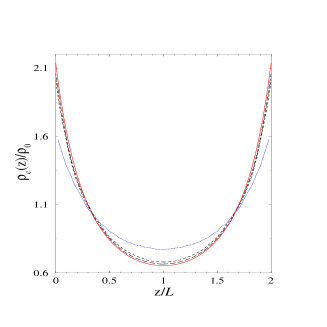
FIG. 1.: Reduced counterion density profiles $\rho^{(0)}_{c}(z)/\rho_{0}$ versus reduced distance $z/L$. solid line- PB prediction and simulation result with incorporating Lekner summation method. Both data do coincide on the same curve, long-dashed line- result of simulation in HSG, dashed line- result of PRI simulation with ${\cal N}=2$, dotted line- result of MIC simulation.

The corresponding MD simulation data were obtained with 600 counterions in the cell using various boundary conditions. As expected, the PB theory coincides with the Lekner summation method which treats best the long-range nature of the Coulomb interactions. In HSG the counterionic profiles are also very similar to the Lekner summation while the MIC deviates significantly. The MIC can already be improved significantly if ${\cal N}=2$ periodic repeated images are included. In conclusion, the agreement between Lekner summation and HSG justifies the HSG a posteriori and gives evidence that the HSG produces reliable results also for stronger couplings.

V Single macroion between charged plates

Let us now consider a single macroion in the inter-lamellar area. We put the macroion on the $z$-axis, such that its position is at ${\vec{R}}_{1}=(0,0,Z_{1})$. A corresponding schematic picture is given in Fig.2.

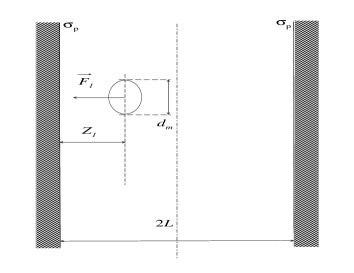
FIG. 2.: Schematic picture for a single macroion between likely charged planes of charge density $\sigma_{p}$, separated by distance $2L$.

The total force acting on the macroion only depends on $Z_{1}$ and points along the $z$-axis. Obviously, for the case $\sigma_{1}=\sigma_{2}=\sigma_{p}$ of symmetric plates considered here, the direct part of the total force, ${\vec{F}}_{j}^{(1)}$, vanishes. For the second (electrostatic) part, simple PB-theory applied to the case of small macroion charge and small macroion diameter yields the following analytical expression for the effective macroion force [58, 6]

$${\vec{F}}_{1}^{PB}=\frac{2Zk_{B}T\gamma_{0}}{qL}\tan\left(\gamma_{0}\left(1-z/L\right)\right){\vec{e}}_{z}$$ (23)

where ${\vec{e}}_{z}$ is the unit vector in $z$-direction and $\gamma_{0}$ is given by (22). Note that only the counterion density stemming from the charged plates has to be inserted in (22) i.e. $\rho_{o}=\frac{\sigma_{p}}{L\mid qe\mid}$. This force pushes the macroion towards the mid-plane, i.e. the wall-particle interaction is repulsive.

The expression (23) will break down, however, for a large macroion diameter $d_{m}$ and for strong macroion-counterion coupling parameter $\Gamma_{mc}$. We have tested the PB-theory against “exact” computer simulation data. For moderate couplings (run B and run C) the results for the total force $F_{1}={\vec{F}}_{1}\cdot{\vec{e}}_{z}$ are shown in Figs.3-4. In Fig.3, a surprising agreement between theory and simulation is obtained despite the fact that the macroion charge is large.

FIG. 3.: Force $F_{1}={\vec{F}}_{1}\cdot{\vec{e}}_{z}$ acting on a single macro-ion versus reduced macro-ion distance $Z_{1}/L$. The force is scaled by the (arbitrary) unit $F_{0}=\frac{Zqe^{2}}{\epsilon{d_{m}^{2}}}$. The system parameters are from run B. The solid line is the prediction from PB theory. The open circles are simulation results in HSG. The statistical error corresponds to the symbol size.

This justifies the theoretical conclusions drawn in Refs. [6, 7] based on PB theory. The deviation between theory and simulation are larger in Fig.4 where the surface charge density was doubled. Here, also the system size dependence (resp. the dependence on the macroion density) was studied in the simulation.

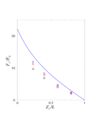
FIG. 4.: Same as Fig.3 but now for run C. Symbols are simulation results in HSG for various macroion number densities: circles: $\rho_{m}=1.17\times 10^{13}cm^{-3}$, squares: $\rho_{m}=2.0\times 10^{12}cm^{-3}$, triangles: $\rho_{m}=1.0\times 10^{12}cm^{-3}$.

As expected the agreement becomes better for a larger system size (resp. for a smaller macroion density) since the theory is constructed formally for vanishing macroion density. In addition, we repeated the calculations for $\rho_{m}=1.17\times 10^{13}cm^{-3}$ (corresp. to the circles in Fig.4) using the PRI method with $N=4$ and got the same results as in HSG. We now enhance the Coulomb coupling by formally reducing the dielectric constant $\epsilon$. For a fixed macroion position at $Z_{1}=d_{m}$, the force $F_{1}$ is shown in Fig.5 for the parameters of run D.

FIG. 5.: Force $F_{1}={\vec{F}}_{1}\cdot{\vec{e}}_{z}$ acting on a single macro-ion versus dielectric constant $\epsilon$ for a fixed position at $Z_{1}=d_{m}$. The force is scaled by the (arbitrary) unit $F_{0}=0.01\frac{Zqe^{2}}{\epsilon{d_{m}^{2}}}$. The parameters of the system are from run D. The solid line is the prediction of PB theory. The crosses are simulation results in HSG.

While the PB theory always predicts a repulsive force, the simulation data are in accordance with theory only for large $\epsilon$ but the force changes its sign for $\epsilon<10$. Hence as expected the theory breaks down for large Coulomb coupling where correlation between the counterions become significant.

For the same run D, the distance-resolved macroion force $F_{1}$ is shown in Fig.6 for a strongly reduced dielectric constant $\epsilon=3.9$. The simulation data were obtained in HSG but confirmed by PRI calculations with ${\cal N}=4$. The electrostatic part $F_{1}^{(2)}={\vec{F}}_{1}^{(2)}\cdot{\vec{e}}_{z}$ and the depletion part $F_{1}^{(3)}={\vec{F}}_{1}^{(3)}\cdot{\vec{e}}_{z}$ are shown separately. $F_{z}^{(3)}$ is always repulsive and increases with decreasing $Z_{1}$, at least if the macroion is not too close to the surface when the counterion depletion between the macroion and the wall induced by the finite counterion core is negligible. This is an expected behavior, since in general there are more counterions close to the walls. The pure electrostatic contribution, $F_{1}^{(2)}$, on the other hand, exhibits a more subtle behavior. If the macroion is close to the midplane, it is repulsive, then it becomes attractive as the macroion is getting closer to the plates.

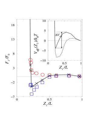
FIG. 6.: Same as Fig.3 but now for run D, $\epsilon=3.9$, and for a force unit of $F_{0}=0.1\frac{Zqe^{2}}{\epsilon{d_{m}^{2}}}$. The crosses are simulation data in HSG for the total force $F_{1}$, the squares (resp. circles) are simulation data the electrostatic part $F_{1}^{(2)}$ (resp. the depletion part $F_{1}^{(3)}$).The line is a guide to the eye for the total force. The inset shows the effective potential in units of $k_{B}T$ versus reduced macro-ion distance $Z_{1}/L$ together with the energy barrier $\Delta V_{eff}$. The solid line is for run D with $\epsilon=3.9$, dashed line is for run E.

As a function of macroion distance, the total force $F_{1}$ is repulsive, attractive and becomes repulsive again. For small separations (which are still larger than the microscopic counterionic core) the force is dominated by the repulsive depletion force. Hence the macroion has got three equilibrium positions, two of them are stable, namely the midplane and a position in the vicinity of the plate. In order to extract more information, we have calculated the effective wall-particle potential defined by

$$V_{eff}(Z_{1})=-\int_{0}^{Z_{1}}F_{1}(h)dh$$ (24)

by integrating our data with respect to the macroion altitude $h$. This quantity is shown as an inset in Fig.6. One first sees that the global minimum is in the vicinity of the walls. Furthermore the barrier height $\Delta V_{eff}$ to escape from there is about $8k_{B}T$. This implies that the time for a colloidal particle to escape from the position close to the surface is roughly $\tau_{0}\exp\left(\Delta V_{eff}/k_{B}T\right)=e^{8}\tau_{0}\approx 3000\tau_{0}$ [59, 60] where $\tau_{0}$ is a Brownian time scale governing the decay of dynamical correlations of the macroion. It can also be seen that, for a doubled surface charge (run E), the height of barrier increases.

A similar behaviour occurs for another parameter combinations (run G), see Fig.7, corresponding to aqueous suspensions of micelle-sized macroions. It hence seems to be a generic feature of the primitive model for strong Coulomb coupling.

FIG. 7.: Same as Fig.6 but now for run G and for a force unit of $F_{0}=0.1\frac{Zqe^{2}}{\epsilon{d_{m}^{2}}}$. The squares are simulation results for the total force in HSG for $\sigma_{p}=1.19\times 10^{14}{e\over cm^{2}}$, while the circles are for $\sigma_{p}=2.38\times 10^{14}{e\over cm^{2}}$. The lines are a guide to the eye. The inset shows the effective potential in units of $k_{B}T$ versus reduced macro-ion distance $Z_{1}/L$. The dashed line is for $\sigma_{p}=1.19\times 10^{14}{e\over cm^{2}}$, the solid line is for $\sigma_{p}=2.38\times 10^{14}{e\over cm^{2}}$.

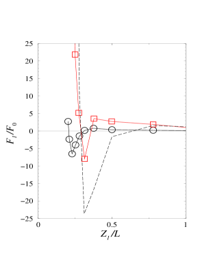
FIG. 8.: Effective force $F_{1}={\vec{F}}_{1}\cdot{\vec{e}}_{z}$ (circles) and gradient of the potential energy $\bar{F}_{1}={\vec{\bar{F}}}_{1}\cdot{\vec{e}}_{z}$ (squares) versus reduced macro-ion distance $Z_{1}/L$ for run K. The unit of the force is $F_{0}=0.1{{Zqe^{2}}\over{\epsilon d_{m}^{2}}}$. the lines are a guide to the eye. The dashed line are data from Ref.[60]

We note that the barrier height $\Delta V_{eff}$ is about $70k_{B}T$ which implies a very large escape time. Finally we show for a certain parameter combination (run K) which was also used in Ref.  [61] that the averaged force ${\vec{F}}_{1}$ differs from the gradient of the averaged potential energy ${\vec{\bar{F}}}_{1}$. As in Ref.  [61], the system consists of a single macroion in a planar slit of width $5d_{m}$, with one charged and one neutral wall. Results are given in Fig.8. We conclude that the forces behave even qualitatively different. The average force ${\vec{F}}_{1}$ is a short-range attractive force which becomes repulsive only for touching macroion configurations. Contrary to that, the force ${\vec{\bar{F}}}_{1}$ is repulsive up to distance about $d_{m}/2$ from the wall surface. Note that our data actually differ from those of Ref. [61] due to the early truncation of the Coulomb interaction performed there.

VI Two macro-ions between plates

We finally consider two equally charged macroions at the positions ${\vec{R}}_{1}=(X_{1},Y_{1},Z_{1})$ and ${\vec{R}}_{2}=(X_{2},Y_{2},Z_{2})$ confined between plates. A schematic picture is given in Fig.9.

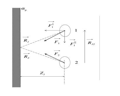
FIG. 9.: Schematic picture for the macroion pair near a charged wall of surface charge density $\sigma_{p}$. For the sake of clarity, the position of second wall is omitted. The different forces are shown for the case of a mutual attraction.

In order to reduce the parameter space, we assume for simplicity that both macroions have the same altitude $Z_{1}=Z_{2}$. The distance between the macroion centers is $R_{12}=\mid{\vec{R}}_{1}-{\vec{R}}_{2}\mid$ where the difference vector ${\vec{R}}_{12}={\vec{R}}_{1}-{\vec{R}}_{2}$ is in the $xy$-plane. We assume that only one of the walls is charged and that the second wall is neutral. This gives us the possibility to simulate higher surface charge densities. Also for strong coupling, the counterions of the two different walls are practically decoupled such that the set-up with a single charged wall is not expected to differ much from the symmetrical set-up. The total force acting on the two macroions can be split into a part pointing in $z$-direction and another contribution pointing along ${\vec{R}}_{12}$. Hence we write ${\vec{F}}_{j}={\vec{F}}^{\|}_{j}+{\vec{F}}^{\bot}_{j}$ defining ${\vec{F}}^{\|}_{j}=\left({\vec{F}}_{j}\cdot{\vec{R}}_{12}\right)\cdot{\vec{R}}_{12}/R_{12}^{2}$ and ${\vec{F}}^{\bot}_{j}=\left({\vec{F}}_{j}\cdot{\vec{e}}_{z}\right)\cdot{\vec{e}}_{z}$ for $j=1,2$. Clearly, ${\vec{F}}^{\bot}_{1}={\vec{F}}^{\bot}_{2}$, and ${\vec{F}}^{\|}_{1}=-{\vec{F}}^{\|}_{2}$.

It is instructive to compare these force to the DLVO bulk theory which yields

$${\vec{F}}^{DLVO}_{1}= \frac{{Z}^{2}e^{2}\exp{((d_{m}-R_{12})/\lambda_{D})}}{\epsilon R_{12}(1+{d_{m}/2\lambda_{D}})^{2}}$$ (26)

$$\times\left({1\over R_{12}}+{1\over\lambda_{D}}\right){{\vec{R}}_{12}\over R_{12}}$$

Here the Debye screening length $\lambda_{D}$ is given by eq.(20), where $\rho_{0}$ corresponds to the counterion number density coming only from the macroions, $\rho_{0}={Z\over{q}}\rho_{m}$. One can also modify the DLVO theory by admitting screening also from the counterions stemming from the wall assuming they follow a Poisson-Boltzmann density profile. This yields the PB force [6, 7]

$${\vec{F}}^{PB}_{1}=({\vec{F}}^{PB}_{1})^{\|}+({\vec{F}}^{PB}_{1})^{\bot}$$ (27)

where we get for the parallel part of the force

$$({\vec{F}}_{1}^{PB})^{\|}= \frac{{Z}^{2}e^{2}\exp{(-R_{12}/\lambda_{D}(Z_{1}))}}{\epsilon R_{12}}$$ (29)

$$\times\left({1\over R_{12}}+{1\over\lambda_{D}(Z_{1})}\right){{\vec{R}}_{12}\over R_{12}}.$$

The perpendicular part of the force is

$$({\vec{F}}^{PB}_{1})^{\bot}= {\vec{F}}_{1}^{PB}-\frac{{Z}^{2}e^{2}}{\epsilon}\frac{\lambda_{D}(Z_{1})\gamma_{0}^{3}}{L^{3}}$$ (31)

$$\times\frac{\tan\left(\gamma_{0}(1-Z_{1}/L)\right)}{\cos^{2}\left(\gamma_{0}(1-Z_{1}/L)\right)}{\vec{e}}_{z}$$

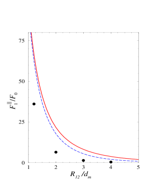
FIG. 10.: Parallel part of the effective force acting onto a macroion pair, $F^{\|}_{1}={\vec{F}}^{\|}_{1}\cdot{{\vec{R}}_{12}/R_{12}}$, versus reduced interparticle distance $R_{12}/d_{m}$. The unit of the force is $F_{0}=\left(\frac{Z^{2}e^{2}}{\epsilon{d_{m}^{2}}}\right)\,\times 10^{-2}$. The parameters of system are from run L and for an altitude of macroions of $Z_{1}=0.6d_{m}$. The solid line is the bulk DLVO theory, the dashed line is the Poisson-Boltzmann theory (29) and the points are simulation results in HSG. The statistical error corresponds to the symbol size.

The space dependent Debye screening length is

$$\lambda_{D}(Z_{1})=\left(4\pi\lambda_{B}\left({Z\over q}\rho_{m}+\rho_{c}^{PB}(Z_{1})\right)\right)^{-\frac{1}{2}}$$ (32)

Here $\rho_{c}^{PB}(z)$ and ${\vec{F}}_{1}^{PB}$ are given by Eqns. (21) and (23). Contrary to the bulk DLVO force, the PB force has an additional perpendicular part for a pair of particles (second term in (31)). This additional force is attractive. Still the total perpendicular force (31) is always repulsive.

For the parameters of run L corresponding to weak coupling, simulation results for $F^{\|}_{1}={\vec{F}}^{\|}_{1}\cdot{{\vec{R}}_{12}/R_{12}}$ are shown in Fig.10.

The solid line corresponds to the bulk DLVO force, and the dashed line is the Poisson-Boltzmann result. The force is repulsive both in theory and simulation, but the theories overestimate the force significantly. As expected the Poisson-Boltzmann approach yields better agreement than DLVO bulk theory.

Results for $F^{\|}_{1}$ for stronger coupling (runs M and N) are displayed in Figs.11-12.

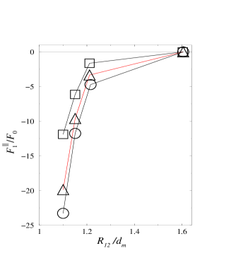
FIG. 11.: Same as Fig.10 but now for run M and $F_{0}=\left(\frac{Z^{2}e^{2}}{\epsilon{d_{m}^{2}}}\right)\,\times 10^{-3}$. Simulation results are shown for three different surface charges: squares: $\sigma_{p}=0{e\over cm^{2}}$, triangles: $\sigma_{p}=2.98\times 10^{11}{e\over cm^{2}}$, circles: $\sigma_{p}=5.95\times 10^{11}{e\over cm^{2}}$. The lines are a guide to the eye.

For a neutral wall, the interaction force between macroions is already attractive. With increasing surface charge the attraction between macroions becomes stronger. Clearly this attraction is neither contained in DLVO theory nor in the Poisson-Boltzmann approach (29).

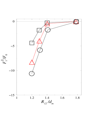
FIG. 12.: Same as Fig.11 but now for run N and for $Z_{1}=0.7\,d_{m}$. Results are shown for three different surface charges: squares: $\sigma_{p}=0{e\over cm^{2}}$, triangles: $\sigma_{p}=1.19\times 10^{14}{e\over cm^{2}}$, circles: $\sigma_{p}=2.38\times 10^{14}{e\over cm^{2}}$.

In Fig.13 we fixed the macroion distance and calculated $F^{\|}_{1}$ and the force perpendicular to the plates, $F^{\bot}_{1}={\vec{F}}^{\bot}_{1}\cdot{\vec{e}}_{z}$ versus altitude $Z_{1}$ for run N.

FIG. 13.: Parallel $F^{\|}_{1}={\vec{F}}^{\|}_{1}\cdot{{\vec{R}}_{12}/R_{12}}$ ( squares) and perpendicular $F^{\bot}_{1}={\vec{F}}^{\bot}_{1}\cdot{\vec{e}}_{z}$ (circles) parts of effective force versus reduced altitude $Z_{1}/d_{m}$ for fixed interparticle spacing $R_{12}=1.2\,d_{m}$. The unit of the force $F^{\|}_{1}$ is $F_{0}=\left(\frac{Z^{2}e^{2}}{\epsilon{d_{m}^{2}}}\right)\,\times 10^{-3}$, and for the force $F^{\bot}_{1}$ is $F_{0}^{*}=\left(\frac{Z^{2}e^{2}}{\epsilon{d_{m}^{2}}}\right)\,\times 10^{-2}$. The surface charge density is $\sigma_{p}=2.38\times 10^{14}{e\over cm^{2}}$. The inset shows the effective potential in units of $k_{B}T$ versus reduced macro-ion distance $Z_{1}/d_{m}$.

There is attraction. Both the interparticle attraction and the wall-particle attraction become stronger in the vicinity of the plate. The effective wall-particle interaction potential for the perpendicular part is shown as an inset in Fig.13. Note that the minimum of $V_{eff}$ is much more than twice as large as in the single macroion case (compare to inset in Fig.7, solid line). Thus, a pair of macroions near a planar surface is more stable than a single macroion. This is also evident from the results for run N shown in Fig.14.

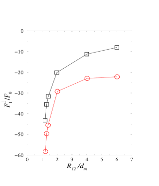
FIG. 14.: Perpendicular part of the effective force acting onto a macroion pair, $F^{\bot}_{1}={\vec{F}}^{\bot}_{1}\cdot{\vec{e}}_{z}$ in units of $F_{0}=\left(\frac{Z^{2}e^{2}}{\epsilon{d_{m}^{2}}}\right)\,\times 10^{-3}$ versus dimensionless interparticle distance $R_{12}/d_{m}$. The parameters of system are from run N and the altitude of macroions is fixed to $Z_{1}=0.7\,d_{m}$. Simulation results are shown for two different surface charges: squares: $\sigma_{p}=1.19\times 10^{14}{e\over cm^{2}}$, circles: $\sigma_{p}=2.38\times 10^{14}{e\over cm^{2}}$.

Again there is attraction towards the plate for varied $R_{12}$ and fixed $Z_{1}$. The attraction becomes stronger if the interparticle distance is decreasing. This shows that the attraction between the wall and a single macroion discussed in chapter V is stable and even enhanced if more macroions are close to the wall. This leads us to the final conclusion that the macroions will assemble on top of the surface forming two-dimensional colloidal layers.

VII Conclusions

We have simulated the effective force between macroions confined in a slit-geometry. An effective attraction was found for strong Coulomb coupling. In particular, the effective potential of a single macroion confined between two parallel charged plates was found to have two stable minima where the total force vanishes: the first is in the mid-plane, the second close to the walls. This result was confirmed for two macroions. In this case the attraction towards the walls was even stronger than for a single macroion. Our most important conclusion is that the attractive force will result in two-dimensional colloidal layers on top of the plates. As the depth of the attractive potential is larger than $k_{B}T$, these layers possess a large life-time with respect to thermal fluctuations. The layers should be crystalline as the interparticle interaction is also attractive. This can explain at least qualitatively the long-lived metastable crystalline layers found in recent experiments on confined samples of charge colloidal suspensions [32, 33].

We want to add some remarks: First, our parameters are actually different form those describing the experiments. The main difference is the high surface charge of the glass plates within an area spanned by a typical macroion separation distance. Such a system cannot be simulated since it requires a huge number of counterions in the simulation box. We have mimicked the high surface charge by dealing with a small dielectric constant, but strictly speaking this corresponds to a different system. Second, the mechanism of our attraction is similar to that proposed recently by us in the bulk case [26]. It only occurs for strong coupling with divalent counterions and is short-ranged. In this respect, it behaves different than in experiment where the attraction was long-ranged. We emphazise again that the depletion force is crucial in the strong coupling parameter regime. Third, our computer simulation data were tested against simple DLVO- or Poisson-Boltzmann-type theories. It would be interesting to use them as benchmark data for more sophisticated theoretical approaches which predict attraction as e.g. the density functional perturbation theory recently proposed by Goulding and Hansen [9]. Finally, in our simulations, we neglected any impurity or added salt ions. Their inclusion increases substantially the number of microscopic particles and would lead to more extensive simulation. A further challenge would be to incorporate image charges properly into the model which requires a non-trivial extension of our approach.

A Definition of forces in Hyper Sphere Geometry

We shortly present here some technical details in HSG within the primitive model. For more details, we refer to Ref. [54].
The charged hard spheres are confined on the surface $S_{3}$ of a 4D hypersphere. Without confinement, in the bulk, the whole surface of the hypersphere is accessible to the particles. Since $S_{3}$ is compact, the total charge in a closed space must be equal to zero. We define a pseudocharge as the association of a point charge $q_{i}$ located at the point say $M$, and a neutralizing background of total charge $-q_{i}$. The position of pseudocharge is specified by the 4D spherical coordinates $(\alpha,\theta,\varphi)$ (see Fig. 15).

FIG. 15.: Schematic view of the hypersphere (projected to three dimensions) illustrating the angular coordinate $\alpha$.

Then the Cartesian components of the unit vector ${\vec{u}}(M)=\vec{OM}$/$R$ reads

$$u_{1}=\sin{\alpha}\sin{\theta}\cos{\varphi},\,\,u_{2}=\sin{\alpha}\sin{\theta}\sin{\varphi},\,\,$$ (A1)

$$u_{3}=\sin{\alpha}\cos{\theta},\,\,u_{4}=\cos{\alpha}$$ (A2)

Here $R$ is the hypersphere radius, $O$ is the center of the hypersphere and the angle $\alpha$ determines the distance $R\alpha$ from north pole, see Fig. 15. The distance between two pseudocharges $q_{i}$ (at point $M$) and $q_{j}$ (at point $N$) is measured along the geodesic line joining these points

$$r_{MN}=R\,\gamma,$$ (A3)

where $\gamma$ is the angle between vectors $\vec{OM}$ and $\vec{ON}$,

$$\gamma=\arccos{\frac{\vec{OM}\,\cdot\vec{ON}}{R^{2}}}$$ (A4)

The Coulomb force $\vec{F}_{ij}$ between pseudocharge $q_{i}$ and pseudocharge $q_{j}$ is

$${\vec{F}}_{ij}=\frac{q_{j}\,q_{i}}{\epsilon\pi R^{2}}\left(\cot{\gamma}+\frac{\pi-\gamma}{\sin^{2}{\gamma}}\right){\vec{e}}_{\gamma}(N).$$ (A5)

Here $\vec{e}_{\gamma}(N)$ denotes the unit vector tangent to geodesic $MN$ at point $N$

$$\vec{e}_{\gamma}=-\frac{1}{\sin{\gamma}}{\vec{u}}(M)+\cot{\gamma}\,\,{\vec{u}}(N)$$ (A6)

For short distances $r_{MN}$, there is the hard core repulsion. A hard sphere of diameter $d_{i}$ ($i=c,m$) centered around the point $M$ on $S_{3}$ is defined as the set of points $M_{0}$ such that $R\,\gamma_{MM_{0}}=R\,\arccos{\frac{\vec{OM}\,\cdot\vec{OM_{0}}}{R^{2}}}<d_{i}/2$. Thus, the hard sphere potential between two pseudocharge is defined by

$$U_{ij}=\left\{\begin{array}[]{ll}\infty&\text{if}\>\gamma\langle\frac{d_{i}+d_{j}}{2R},\,\,i,j=c,m\\ 0&\text{otherwise.}\end{array}\right.$$ (A7)

Let us now consider the mixed hard sphere system to be confined between two charged walls. On $S_{3}$ geometry it corresponds to the two charged lamellae, parallel to each other, localized symmetrically on opposite side of the equator (see Fig.(16)).

FIG. 16.: Schematic view of the hypersphere (projected to three dimensions) illustrating a situation with two parallel charged interfaces.

They result from a conical section of the hypersphere, with angular apertures equal to $\alpha_{N}$ for north lamellar and $\alpha_{S}=\pi-\alpha_{N}$ for south lamellar. The area of each lamellar is   $S_{p}=4\pi R^{2}\sin^{2}{\alpha_{N}}$ and the volume confined between lamellae is given by

$$V(\alpha_{N})=\pi R^{3}(2\alpha_{N}-\sin{2\alpha_{N}})$$ (A8)

Then the separation distance between lamellar is $D=R(\pi-2\alpha_{N})$. For the symmetrical case considered in this paper, when both lamellar are charged equally with surface charge density $\sigma_{p}$, the charge electroneutrality of simulation cell together with eq. (1) requires

$$N_{p}\,q_{c}\,+\,2\,Q_{p}=0.$$ (A9)

Here $Q_{p}=\sigma_{p}S_{p}$ is the net charge of one lamellar,  $N_{p}$ is the number of counter-ions coming from planes.

Finally, we give the definition of interaction forces. The lamellar-lamellar repulsion force is

$$F_{pp}=\frac{Q_{p}^{2}}{\epsilon\,\pi\,R^{2}}\left(-\cot{\alpha_{N}}+\frac{\alpha_{N}}{\sin^{2}{\alpha_{N}}}\right).$$ (A10)

The ion-ion repulsion ($i=j$) and attraction ($i\neq j$) force is

$$F_{ij}=\frac{q_{j}\,q_{i}}{\epsilon\,\pi\,R^{2}}\left(\cot{\gamma}+\frac{\pi-\gamma}{\sin^{2}{\gamma}}\right),$$ (A11)

here $\gamma$ is given by (A4) and the particles $i$ and $j$ are at points $M$ and $N$, $i,j=m,c$. The ion-lamellar repulsion ($i=m$) and attraction ($i=c$) force is

$$F_{ip}=\frac{Q_{p}\,q_{i}}{\epsilon\,\pi\,R^{2}}\left(\cot{\alpha_{i}}+\frac{\pi\,-\alpha_{i}}{\sin^{2}{\alpha_{i}}}\right).$$ (A12)

for the upper lamella and

$$F_{ip}=\frac{Q_{p}\,q_{i}}{\epsilon\,\pi\,R^{2}}\left(\cot{\alpha_{i}}-\frac{\alpha_{i}}{\sin^{2}{\alpha_{i}}}\right).$$ (A13)

for the second lamella. The direction of the forces is always along the geodesic line.

The lamellar-ion hard core repulsion becomes

$$U_{ip}=\cases{\infty&for $\alpha_{i}<\alpha_{N}+d_{i}/2R,\,\,i=c,m$\cr 0&otherwise\cr}$$ (A14)

B equation of motion for single counter-ion in hyperspherical geometry

In this section we translate Newton equation of motion onto HSG for a counterion in an external electrical field created by charged planes, other counterions and fixed macroions. First of all, let us define the displacement of counterion at point $M$ on $S_{3}$. The differential $d\,\vec{OM}$ of vector $\vec{OM}$ ($M$ remaining on the surface of the hypersphere) is

$$d\,\vec{OM}=R\,d\alpha\,\vec{e}_{\alpha}+R\,\sin{\alpha}\,d\theta\,\vec{e}_{\theta}+R\,\sin{\alpha}\,\sin{\theta}\,\vec{e}_{\varphi}$$ (B1)

where the unit vectors [$\vec{e}_{\alpha},\vec{e}_{\theta},\vec{e}_{\varphi}$] given by

$$\vec{e_{\alpha}} = (\cos{\alpha}\sin{\theta}\cos{\varphi},\cos{\alpha}\sin{\theta}\sin{\varphi},$$

$$\cos{\alpha}\cos{\theta},-\sin{\theta}),$$

$$\vec{e_{\theta}}=(\cos{\theta}\cos{\varphi},\cos{\theta}\sin{\varphi},-\sin{\theta},0),$$ (B2)

$$\vec{e_{\varphi}}=(-\sin{\varphi},\cos{\varphi},0,0).$$

constitute an orthogonal frame at point $M$. For the kinetic energy in terms of the variables ($\alpha,\theta,\varphi$) we get

$$T= \frac{mv^{2}}{2}=\frac{m}{2}\left(\frac{d\vec{OM}}{dt}\right)^{2}$$ (B4)

$$=\frac{m}{2}\left(R^{2}\,{\dot{\alpha}}^{2}+R^{2}\,{\sin{\alpha}}^{2}\,{\dot{\theta}}^{2}+R^{2}\,{\sin{\alpha}}^{2}\,{\sin{\theta}}^{2}\,{\dot{\varphi}}^{2}\right)$$

For the potential energy we have relations

$$-\frac{\partial{U}}{\partial{\alpha}}=R\,F_{\alpha},\,\,\, -\frac{\partial{U}}{\partial{\theta}}=R\,\sin{\alpha}\,F_{\theta},\,\,\,$$ (B6)

$$-\frac{\partial{U}}{\partial{\varphi}}=R\,\sin{\alpha}\,\sin{\theta}\,F_{\alpha}$$

Now let us put Eqs.(B4) and (B6) into Lagrange equations

$$\frac{d}{dt}\,\frac{\partial{T}}{\partial{v_{i}}}-\frac{\partial{T}}{\partial{x_{i}}}= \sum_{j=1}^{N_{c}}\frac{\partial{U_{ij}}}{\partial{x_{i}}}+\sum_{k=1}^{N_{m}}\frac{\partial{U_{ki}}}{\partial{x_{i}}}$$ (B8)

$$+\sum_{l=1}^{2}\frac{\partial{U_{li}}}{\partial{x_{i}}}\>\>\>(i=\alpha,\theta,\varphi\>\>\text{and}\>\>x_{i}=i)$$

where on the right hand side the first term arises from all counterions, the second term is the macroionic attraction, the last term is due to plane attraction. The Newton equations of counterion motion reads as follows

$$\ddot{\alpha}=\sin{\alpha}\,\cos{\alpha}\,\left({\dot{\theta}}^{2}+{\sin^{2}{\theta}}{\dot{\varphi}}^{2}\right)+\frac{1}{m\,R}\,F_{\alpha},\,$$ (B9)

$$\frac{d}{dt}\left({\sin^{2}{\alpha}}\,\dot{\theta}\right)={\sin^{2}{\alpha}}\,\sin{\theta}\,cos{\theta}\,{\dot{\varphi}}^{2}+\frac{\sin{\alpha}}{m\,R}\,F_{\theta},$$ (B10)

$$\frac{d}{dt}\left({\sin^{2}{\alpha}}\,{\sin^{2}{\theta}}\,\dot{\varphi}\right)=\frac{\sin{\alpha}\,\sin{\theta}}{m\,R}\,F_{\varphi}.$$ (B11)

We note that $(F_{\alpha},F_{\theta},F_{\varphi})$ are the components of total force arising from all other counter-ions, planes and macro-ions. The equations of motion Eq.(B9)-(B11) have been solved in a way similar to that described in [62].

The spherical components $(F_{\alpha},F_{\theta},F_{\varphi})$ of vector $\vec{F}$ are connected with the 4D force eq.( A5) by the following relations

$$F_{\alpha}=F_{1}\cos{\alpha}\sin{\theta}\cos{\varphi} + F_{2}\cos{\alpha}\sin{\theta}\sin{\varphi}$$

$$+ F_{3}\cos{\alpha}\cos{\theta}-F_{4}\sin{\theta},$$

$$F_{\theta}=F_{1}\cos{\theta}\cos{\varphi}+F_{2}\cos{\theta}\sin{\varphi}-F_{3}\sin{\theta},$$ (B12)

$$F_{\varphi}=-F_{1}\sin{\varphi}+F_{2}\cos{\varphi}.$$

REFERENCES

- [1] To whom correspondence should be addressed. E-mail: allahyar@thphy.uni-duesseldorf.de
- [2] G.M.Kepler, S.Fraden, Phys.Rev.Letters 73, 356 (1994).
- [3] J.C.Crocker, D.G.Grier, Phys.Rev.Letters 77, 1897 (1996).
- [4] D.G.Grier, Nature 393 621 (1998).
- [5] B.V.Derjaguin, L.Landau, Acta Physicochimica (USSR) 14, 633 (1941); E.J.Verwey, J.Th.G.Overbeek, Theory of the Stability of Lyophobic Colloids,(Elsevier, Amsterdam, 1948).
- [6] A.Denton, H.Löwen, Thin Solid Films 330, 7 (1998).
- [7] J.Chakrabarti, H.Löwen, Phys. Rev. E 58, 3400 (1998).
- [8] H.Löwen, E. Allahyarov, J. Phys. Condensed Matter 10, 4147 (1998).
- [9] D.Goulding, J.P.Hansen, accepted in Europhysics Letters; D.Goulding, J.P.Hansen, New Approaches to Problems in Liquid State Theory Inhomogeneities and Phase Separation in Simple, Complex and Quantum Fluids. Carlo Caccamo, Jean-Pierre Hansen, George Stell, Kluwer (1999).
- [10] R. Tehver, F. Ancilotto, F. Toigo, J. Koplik, J. R. Banavar, Phys. Rev. E 59, R1335 (1999).
- [11] W.R.Bowen, A.O.Sharif, Nature 393, 663 (1998).
- [12] M. Ospeck, S. Fraden, J. Chem. Phys. 109, 9166 (1998).
- [13] J. C. Neu, Phys. Rev. Letters 82, 1072 (1999).
- [14] K. S. Schmitz, “Macroions in Solution and Colloidal Suspension”, VCH Publishers, Inc,, New York, 1993.
- [15] E. Chang, D. Hone, J. Physique (France) 49 25 (1988).
- [16] S. Tandon, R. Kesavamoorthy, S. A. Asher, J. Chem. Phys. 109, 6490 (1998).
- [17] D.Goulding, J.P.Hansen, Molecular Physics 95, 649 (1998).
- [18] B. V. R. Tata, E. Yamahara, P. V. Rajamani, N. Ise, Phys. Rev. Letters 78, 2660 (1997); J. Yamanaka, H. Yoshida, T. Koga, N. Ise, T. Hashimoto, Phys. Rev. Letters 80, 5806 (1998); H.Yoshida, J.Yamanaka, T.Koga, T.Koga, N.Ise, T.Hashimoto, Langmuir 15, 2684 (1999).
- [19] R. F. Considine, R. A. Hayes, R. G. Horn, Langmuir 15, 1657 (1999).
- [20] J. A. Weiss, A. E. Larsen, D. G. Grier, J. Chem. Phys. 109, 8659 (1998).
- [21] Y. Levin, Physica A 265, 432 (1999).
- [22] R. Netz, H. Orland, Europhysics Letters 45, 726 (1999).
- [23] B.I.Shklovskii, Phys.Rev.Letters 82, 3268 (1999).
- [24] E. Del Giudice, G. Preparata, Modern Physics Letters B 12, 881 (1998).
- [25] M. Tokuyama, Phys. Rev. E 59, R2550 (1999).
- [26] E.Allahyarov, I.D’Amico, H.Löwen, Phys.Rev.Letters 81, 1334 (1998).
- [27] N. Grønbech-Jensen, K. M. Beardmore, P. Pincus, Physica A 261, 74 (1998).
- [28] A. P. Lyubartsev, J. X. Tang, P. A. Janmey, L. Nordenskiöld, Phys. Rev. Letters 81, 5465 (1998).
- [29] R.van Roij, J.P.Hansen, Phys.Rev.Letters 79, 3082 (1997); R.van Roij, M. Dijkstra, J.P.Hansen, Phys.Rev. E 59, 2010 (1999).
- [30] H. Graf, H. Löwen, Phys. Rev. E 57, 5744 (1998).
- [31] P. Linse, J. Chem. Phys. 110, 3493 (1999).
- [32] A. E. Larsen, D. G. Grier, Phys. Rev. Letters 76, 3862 (1996).
- [33] A.E.Larsen, D.G.Grier, Nature 385, 230 (1997).
- [34] J.A.Weiss, D.W.Oxtoby, D.G.Grier, J.Chem.Phys. 103, 1180 (1995).
- [35] H. Löwen, J. P. Hansen, P. A. Madden, J. Chem. Phys. 98, 3275 (1993).
- [36] E. Allahyarov, H. Löwen, S. Trigger, Phys. Rev. E 57, 5818 (1998).
- [37] H. Löwen, Progr. Colloid Polym. Sci. 110, 12 (1998).
- [38] S.W.de Leeuw, J.W.Perram, E.R.Smith, Proc.R.Soc. London Ser.A 373, 27 (1980); A 373, 57 (1980).
- [39] J.P.Hansen, Phys.Rev.A 8, 3096 (1973); E.L.Pollock, J.P.Hansen, ibid 8, 3110 (1973).
- [40] J.P.Valleau, L.K.Cohen, J.Chem.Phys. 72, 5935 (1980); J.P.Valleau, L.K.Cohen, D.N.Card, ibid. 72, 5942 (1980).
- [41] J.W.Halley, J.Hautman, A.Rahman, Y.-J.Rhee, Phys.Rev.B 40, 36 (1989).
- [42] J.Lekner, Physica A 176, 485 (1991).
- [43] N.Grønbech-Jensen, G.Hummer, K.Beardmore, Molecular Physics 92, 941 (1997).
- [44] R.J.Mashl, N.Grønbech-Jensen, J.Chem.Phys. 109, 4617 (1998), R.J.Mashl, N.Grønbech-Jensen, ibid 110, 2219 (1999).
- [45] See e.g.: K.W.Kratky, J.Comp.Physics 37, 205 (1980).
- [46] J.P.Hansen, D.Levesque, J.J.Weis, Phys.Rev.Letters 43, 979 (1979).
- [47] J.M.Caillol, D.Levesque, J.J.Weis, J.P.Hansen, J.Stat.Physics 28, 325 (1982).
- [48] J.M.Caillol, D.Levesque, J.J.Weis, Molecular Physics 44, 733 (1981).
- [49] K.W.Kratky, W.Schreiner, J.of.Comp.Physics 47, 313 (1982).
- [50] J.M.Caillol, D.Levesque, Phys.Rev.B 33, 499 (1986).
- [51] W.Schreiner, K.W.Kratky, Molecular Physics 50, 434 (1983).
- [52] J.Tobochnik, P.M.Chapin, J.Chem.Phys. 88, 5824 (1988).
- [53] J.M.Caillol, J.Chem.Phys. 99, 8953 (1993).
- [54] R.J.-M.Pellenq, J.M.Caillol, A.Delville, J.Phys.Chem.B 101, 8584 (1997); A.Delville. R.J.-M.Pellenq, J.M.Caillol, J.Chem.Phys. 106, 7275 (1997); see references therein.
- [55] M. J. Stevens, M. O. Robbins, Europhys. Letters 12, 81 (1990).
- [56] J. P. Valleau, R. Ivkov, G. M. Torrie, J. Chem. Phys. 95, 520 (1991).
- [57] I.Rouzina, V.A.Bloomfield, J.Phys.Chem. 100, 9977 (1996).
- [58] S.Engström, H.Wennerström, J.Phys.Chem. 82, 2711 (1978).
- [59] W. B. Russel, D. A. Saville, W. R. Schowalter, “Colloidal Dispersions”, Cambridge University Press, Cambridge, pp 267-269, 1989.
- [60] S. Sauer, H. Löwen, J. Phys. Condensed Matter 8, L803 (1996).
- [61] B.Svensson, B.Jönsson, Chem.Phys.Letters 108, 580 (1984).
- [62] J.Bajoras, D.Levesque, B.Quentrec, Phys.Rev.A 7 1092 (1973)