Two-scale competition in phase separation with shear

Abstract

The behavior of a phase separating binary mixture in uniform shear flow is investigated by numerical simulations and in a renormalization group (RG) approach. Results show the simultaneous existence of domains of two characteristic scales. Stretching and cooperative ruptures of the network produce a rich interplay where the recurrent prevalence of thick and thin domains determines log-time periodic oscillations. A power law growth $R(t)\sim t^{\alpha}$ of the average domain size, with $\alpha=4/3$ and $\alpha=1/3$ in the flow and shear direction respectively, is shown to be obeyed.

The application of a shear flow to a disordered binary mixture quenched into a coexistence region greatly affects the phase-separation process [1]. A large anisotropy is observed in typical patterns of domains which appear greatly elongated in the direction of the flow [2]. This behavior has consequences for the rheological properties of the mixture. A rapid strain-induced thickening followed by a gradual thinning regime is observed [3]. Various numerical simulations confirm these observations [4, 5, 6].

In a recent paper [7] we have studied the phase-separation kinetics in the context of a self-consistent approximation, also known as large-$N$ limit. Within this approach the existence of a scaling regime characterized by an anisotropic power-law growth of the average size of domains was established. The segregation process, however, cannot be fully described by this technique because interfaces are absent for large-$N$ [8].

The aim of this letter is to investigate the ordering process by extensive numerical simulations. Our main result concerns the simultaneous existence of two length scales which characterize the thickness of the growing domains. The competition between these scales produces a rich dynamical pattern with an oscillatory behavior due to the cyclical prevalence of one of the two lengths. A power law growth $R(t)\sim t^{\alpha}$ of the average domain size, with $\alpha=4/3$ and $\alpha=1/3$ in the flow and shear direction respectively, is shown to be obeyed by a renormalization group (RG) analysis.

The kinetic behaviour of the binary mixture is described by the Langevin equation

$$\frac{\partial\varphi}{\partial t}+\vec{\nabla}(\varphi\vec{v})=\Gamma\nabla^{2}\frac{\delta{\cal F}}{\delta\varphi}+\eta$$ (1)

where the scalar field $\varphi$ represents the concentration difference between the two components of the mixture [1]. The equilibrium free-energy can be chosen as usual to be

$${\cal F}\{\varphi\}=\int d^{d}x\{\frac{a}{2}\varphi^{2}+\frac{b}{4}\varphi^{4}+\frac{\kappa}{2}\mid\nabla\varphi\mid^{2}\}$$ (2)

where $b,\kappa>0$ and $a<0$ in the ordered phase. $\vec{v}$ is an external velocity field describing plane shear flow with average profile given by

$$\vec{v}=\gamma y\vec{e}_{x}$$ (3)

where $\gamma$ is the shear rate and $\vec{e}_{x}$ is the unit vector in the flow direction. $\eta$ is a gaussian white noise, representing thermal fluctuations, with mean zero and correlation $\langle\eta(\vec{r},t)\eta(\vec{r}^{\prime},t^{\prime})\rangle=-2T\Gamma\nabla^{2}\delta(\vec{r}-\vec{r}^{\prime})\delta(t-t^{\prime})$, where $\Gamma$ is a mobility coefficient, $T$ is the temperature of the fluid, and the symbol $\langle...\rangle$ denotes the ensemble average.

The Langevin equation (1) has been simulated in $d=2$ by first-order Euler discretization scheme. Periodic boundary conditions have been used in the flow direction while in the $y$ direction the point at $(x,y)$ is identified with the point at $(x+\gamma L,y+L)$, where $L$ is the size of the lattice [4]. Lattices with $L=1024,2048,4096$ and space discretization intervals $\Delta x=0.5,1$ were used. In the phase separation process the initial configuration of $\varphi$ is a high temperature disordered state and the evolution of the system is studied in model (1) with $a<0$. Parameterization invariance of (1) allows one to set $\Gamma=|a|=b=\kappa=1$. The structure factor is defined as $C(\vec{k},t)=\langle\varphi(\vec{k},t)\varphi(-\vec{k},t)\rangle$ where $\varphi(\vec{k},t)$ are the Fourier components of $\varphi$. Results will be shown for the case $\gamma=0.0488$, $T=0$, $L=4096$, $\Delta x=1$, $\langle\varphi\rangle=0$. Similar results have been obtained for other values of the parameters.

A sequence of configurations at different values of the strain $\gamma t$ is shown in Fig. 1. After an early time, when well defined domains are forming, the usual bicontinuous structure of phase separating domains starts to be distorted for $\gamma t\gtrsim 1$.

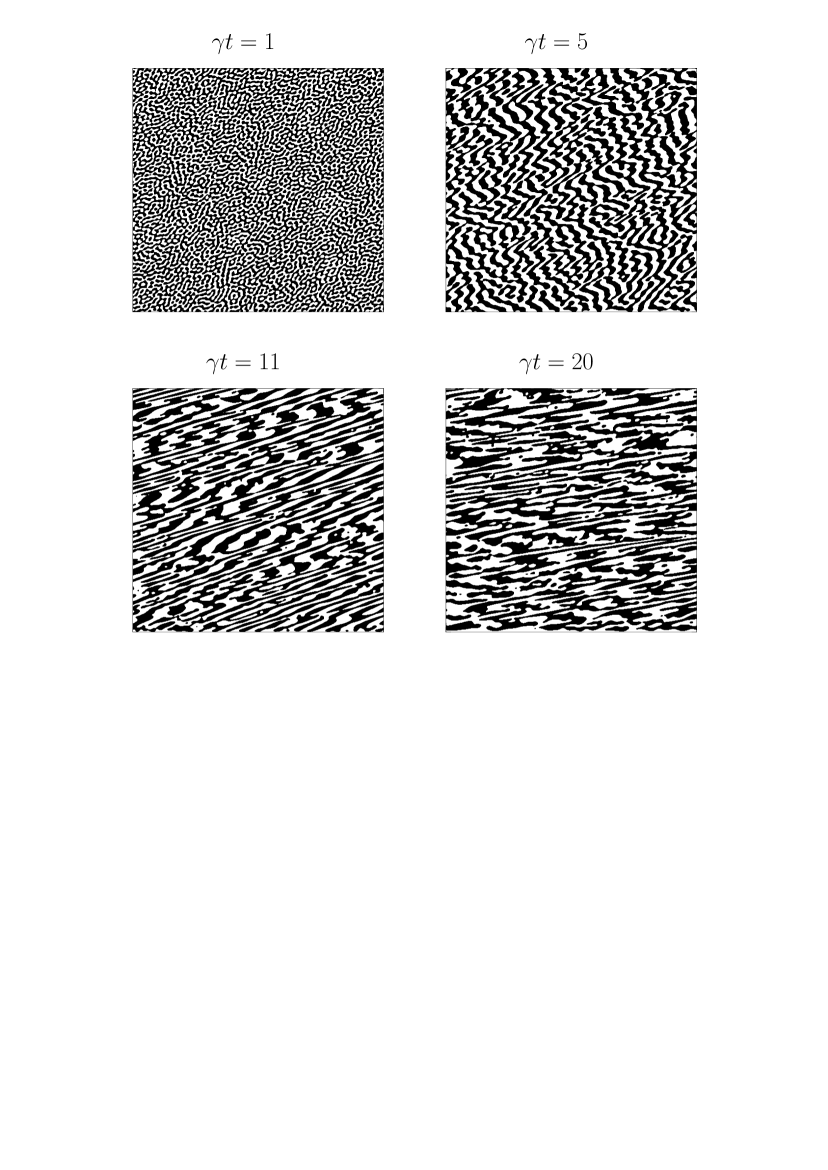
FIG. 1.: Configurations of a portion of $512\times 512$ sizes of the whole lattice are shown at different values of the strain $\gamma t$.

The growth is faster in the flow direction and domains assume the typical striplike shape aligned at an angle $\theta(t)$ with the direction of the shear which decreases with time. As the elongation of the domains increases, nonuniformities appear in the system: Regions with domains of different thickness can be clearly observed at $\gamma t=11$. The evolution at still larger values of the strain is shown for $\gamma t=20$. The domains with the smallest thickness eventually break up and burst with the formation of small bubbles.

A systematic existence of two scales in the size distribution of domains is suggested by the behavior of the structure factor, shown in Fig. 2. At the beginning (see the picture at $\gamma t=0.2$) $C(\vec{k},t)$ exhibits an almost circular shape, corresponding to the early-time regime without sharp interfaces. Then shear-induced anisotropy becomes evident, $C(\vec{k},t)$ is deformed into an ellipse, changing also its profile and, for $\gamma t\gtrsim 1$, four peaks can be clearly observed. The position of each peak identifies a couple of typical lengths, one in the flow and the other in the shear direction. The peaks are related by the $\vec{k}\rightarrow-\vec{k}$ symmetry so that, for each direction, there are two physical lengths. This corresponds to the observation of domains with two characteristic thicknesses, made in Fig. 1.

The dips in the profile of $C(\vec{k},t)$ develop with time until $C(\vec{k},t)$ results to be separated in two distinct foils at $\gamma t\simeq 4$. The evolution of the system until this stage is well described by the solution of the linear part of (1) (letting $b=0$):

$$C(\vec{k},t)=C_{0}\exp^{-\int_{0}^{t}k^{2}(s)(k^{2}(s)-a)ds}$$ (4)

where $\vec{k}(s)=(k_{x},k_{y}+\gamma sk_{x})$ and $C_{0}$ is the structure factor at the initial time [9]. Then non-linear effects become essential in producing the patterns shown in Fig.2 at $\gamma t=11,20$. At $\gamma t=11$ we evaluate the positions of the peaks at $(k_{x},k_{y})=(0.015,0.107)$ and $(k_{x},k_{y})=(0.038,0.23)$. This gives a value around two for the ratio between the characteristic sizes of domains; the same value is found for the ratio between the positions of the two peaks in the hystogram of the domain size distribution. The relative height of the peaks in one of the foils of $C(\vec{k},t)$ can be more clearly seen in Fig.3 where the two maxima are observed to dominate alternatively at the times $\gamma t=11$ and $\gamma t=20$.

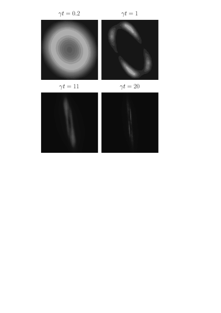
FIG. 2.: The structure factor is shown at different values of the strain $\gamma t$.

The competition between two kinds of domains is a cooperative phenomenon. In a situation like that at $\gamma t=11$, the peak with the larger $k_{y}$ dominates, describing a prevalence of stretched thin domains. When the strain becomes larger, a cascade of ruptures occurs in those regions of the network where the stress is higher and elastic energy is released. At this point the thick domains, which have not yet been broken, prevale and the other peak of $C(\vec{k},t)$ dominates, as at $\gamma t=20$. In the large-$N$ limit the prevalence of one or the other peak has been shown to continue periodically in time [7]. Here we have an indication of a similar behavior, although the observation of the recurrent dominance of the peaks on longer timescales is hardly accessible numerically.

FIG. 3.: The same structure factor of Fig.2 at $\gamma t=11,20$ in a three-dimensional plot.

The hallmarks of this dynamics are found in the behavior of the average size of domains, $R_{x}(t)$ and $R_{y}(t)$, in the flow and shear direction. In our simulations these quantities have been calculated through $R_{x}(t)=(\int d\vec{k}k_{x}^{2}C(\vec{k},t)/\int d\vec{k}C(\vec{k},t))^{-1/2}$, and analogously for $R_{y}(t)$; their behavior is shown in Fig.4. Due to the alternative dominance of the peaks of $C(\vec{k},t)$, $R_{x}$ and $R_{y}$ increase with an oscillatory pattern. The latter reaches a local maximum at the characteristic times $t_{n}$, when $C(\vec{k},t)$ is of the form of Fig. 2 at $\gamma t=20$ and thick domains are more abundant. The time interval $\tau_{n}=t_{n+1}-t_{n}$ between two cascades of ruptures increases exponentially as the phase separation proceeds so that the oscillations appear to be periodic on a logarithmic time scale. This is expected because domains are growing and longer and longer times are required to break them. The following argument simply illustrates the origin of the log-time periodic oscillations: The break up of an elongated domain is caused by the shear flow, which enters Eq. (1) through the last term on the l.h.s., whose magnitude we infere to be proportional to $\tau_{n}^{-1}$. For a sharp interface exposed with an angle $\theta(t)$ to the flow this term is proportional to $\gamma\sin\theta(t)\simeq\gamma\theta(t)\sim\gamma R_{y}(t)/R_{x}(t)$, where the asymptotic smallness of $\theta(t)$ has been taken into account. The RG argument developed below shows that $\gamma R_{y}(t)/R_{x}(t)\sim 1/t$, so that $\tau_{n}\sim t_{n}$ and hence $\ln t_{n}\sim n+cost.$: The rupture events occur periodically in $\ln t$.

Stretching of domains requires work against surface tension and results in an increase $\Delta\eta$ of the viscosity [3, 10]. We calculate the excess viscosity as $\Delta\eta(t)=-\gamma^{-1}\int\frac{d\vec{k}}{(2\pi)^{D}}k_{x}k_{y}C(\vec{k},t)$ [1]. Starting from zero $\Delta\eta$ grows oscillating up to global maximum at $\gamma t\simeq 12$. Then the excess viscosity relaxes to zero in a similar way to what observed in previous simulations [4]. The relative maxima of $\Delta\eta$ are found in correspondence of the minima of $R_{y}$ when the domains are maximally stretched.

In the case without shear the asymptotic kinetics is characterized by dynamical scale invariance, which is reflected by a power law growth $R(t)\sim t^{\alpha}$ of the average size $R(t)$ of domains [8]. The value of the growth exponent $\alpha$ is related to the physical mechanism operating in the separation process and is $\alpha=1/3$ for diffusive growth. In the case with shear the existence of a similar behavior has not been clearly assessed. A stationary state characterized by domains of finite thickness is generally observed in experiments [11]. Only in some experimental realizations the existence of a regime with power law growth has been shown [12, 13].

The self-consistent solution of Eq.(1) shows [7] that a generalized scaling symmetry holds when a shear flow is applied and different exponents are found for the power-law growth of $R_{x}(t)$ and $R_{y}(t)$. However these exponents are correct for models with vectorial order parameter and do not directly apply to the case of a binary mixture [14]. The existence of a scaling symmetry and the actual value of the growth exponents cannot be reliably studied by direct numerical simulation of Eq.(1): This is because, even for the bigger lattice we have used, the fast growth in the $x$-direction makes finite size effects relevant before a full realization of the scaling regime occurs. Moreover, the oscillatory behavior of $R_{x}(t)$ and $R_{y}(t)$ prevents a straightforward computation of the growth exponents, unless the evolution of the system is followed over several decades, which is, presently, impossible. Therefore, in order to infer the actual value of the growth exponents we resort to a RG analysis.

As usual, we define the RG transformation for the Fourier components $\varphi_{\vec{k}}(t)=1/\sqrt{V}\int{d\vec{r}}\varphi(\vec{r},t)e^{i\vec{k}\cdot\vec{r}}$ of the field $\varphi(\vec{r},t)$. They verify the equation

$$\frac{\partial\varphi_{\vec{k}}(t)}{\partial t}-\gamma k_{x}\frac{\partial\varphi_{\vec{k}}(t)}{\partial k_{y}}=-\Gamma k^{2}\frac{\delta{\cal F}}{\delta\varphi_{-\vec{k}}(t)}+\eta_{k}(t)$$ (5)

with $<\eta_{k}(t)\eta_{k^{\prime}}(t^{\prime})>=2T\Gamma k^{2}\delta(t-t^{\prime})\delta(\vec{k}+\vec{k}^{\prime})$. Taking into account the anisotropic growth of domains, we generalize the RG scheme of [15] by considering the change of scale [16]

$$k_{x}\rightarrow k^{\prime}_{x}=k_{x}b^{\alpha_{x}} \qquad k_{y}\rightarrow k^{\prime}_{y}=k_{y}b^{\alpha_{y}},$$ , (6)

$$t \rightarrow t^{\prime}=tb^{-1}$$ (7)

and the field transformation

$$\varphi_{\vec{k}}(t)=b^{\zeta}\varphi^{\prime}_{\vec{k}^{\prime}}(t^{\prime})$$ (8)

where $b$ is the rescaling factor and the meaning of the exponents $\alpha_{x},\alpha_{y},\zeta$ will be clarified in the following. Dimensional analysis implies that the structure factor can be written as

$$C(\vec{k},t)=R_{x}(t)R_{y}(t)f(x,y)$$ (9)

with $x=k_{x}R_{x}(t),y=k_{y}R_{y}(t)$. Its invariance in form with respect to the transformations (7,8) gives $\zeta=(\alpha_{x}+\alpha_{y})/2$. The invariance of the scaling variables $x,y$ under the transformations (7) implies that $\alpha_{x},\alpha_{y}$ correspond to the growth exponents.

FIG. 4.: Evolution of the average domain size in the shear (lower curve) and flow (upper curve) directions. The straight line has slope 4/3.

The dynamical scaling regime is described by a fixed point of the Langevin equation (5) under the set of transformations (7,8) [17]. Generalizing the prescription of [15], we assume that the fixed point hamiltonian ${\cal F}$ verifies the relation

$${\cal F}(b^{\zeta}\varphi^{\prime}_{\vec{k}^{\prime}}(t^{\prime}))=b^{\alpha_{x}}{\cal F}(\varphi^{\prime}_{\vec{k}^{\prime}}(t^{\prime}))$$ (10)

meaning that the main contribution to the free energy is due to the interfaces in the direction of the flow. By inserting (7,8) into (5) and using (10), one obtains a Langevin equation similar in form to (5) with rescaled parameters

$$\frac{1}{\Gamma^{\prime}}=\frac{1}{\Gamma}b^{2\zeta+2\alpha_{y}-1-\alpha_{x}} \qquad\gamma^{\prime}=\gamma b^{\alpha_{y}-\alpha_{x}+1},$$ , (11)

$$T^{\prime} = Tb^{-\alpha_{x}}$$ (12)

A fixed point of the above recursions with $\Gamma,\gamma\neq 0$ is obtained when $\alpha_{y}=1/3,\alpha_{x}=\alpha_{y}+1$, with the temperature being not relevant for the process of phase separation. We observe that a difference between the growth exponents $\Delta\alpha=\alpha_{x}-\alpha_{y}$ in the range $0.8\div 1$ has been measured in [12, 13]. Moreover, the above analysis suggests that, for a constant value of the strain $\gamma t$, the excess viscosity scales as $\Delta\eta\sim\gamma^{-\beta}$ with $\beta=1/3$.

In conclusion, we have studied the phase-separation kinetics of a binary fluid in an uniform shear flow by direct numerical simulation of the constitutive equations and in a RG approach. Results show the simultaneous existence of domains of two characteristic sizes in each direction. The two kind of domains alternatively prevail, because the thicker are thinned by the strain and the thinner are thickened after cascades of ruptures in the network. This mechanism produces an oscillation which decorates the expected power-law growth $R(t)\sim t^{\alpha}$ of the average size of the domains, with $\alpha=4/3$ and $1/3$ in the flow and shear direction, respectively. The oscillations occur on logarithmic time-scale as in models describing propagation of fractures in materials where the releasing of elastic energy is measured [18]. Finally, in a recent paper [19], a first treatment of the effects of hydrodynamics on the phase separation of a binary mixture in uniform shear has been given. It would be interesting to know if and how hydrodynamics affects the global picture described in this letter.

We thank Dino Fortunato and Julia Yeomans for helpful discussions. F.C. is grateful to M.Cirillo and R. Del Sole for hospitality in the University of Rome. F.C. acknowledges support by the TMR network contract ERBFMRXCT980183 and by MURST(PRIN 97).

REFERENCES

- [1] For a review, see A. Onuki, J. Phys.: Condens. Matter 9 6119 (1997).
- [2] T. Hashimoto, K. Matsuzaka, E. Moses, and A. Onuki, Phys. Rev. Lett. 74 126 (1994).
- [3] A.H. Krall, J.V. Sengers, and K. Hamano, Phys. Rev. Lett. 69 1963 (1992).
- [4] T. Ohta, H. Nozaki, and M. Doi, Phys. Lett. A 145 304 (1990); J. Chem. Phys. 93 2664 (1990).
- [5] D.H. Rothman, Europhys. Lett. 14 337 (1991).
- [6] P. Padilla and S. Toxvaerd, J. Chem. Phys. 106 2342 (1997).
- [7] F. Corberi, G. Gonnella, and A. Lamura, Phys. Rev. Lett. 81, 3852 (1998).
- [8] See, e.g., A.J. Bray, Adv. in Phys. 43 357 (1994).
- [9] This solution is obtained by applying the method of characteristics (See, e.g., R. Courant and D. Hilbert, “Methods of mathematical Physics”, J. Wiley Interscience Publ. 1966). Further details will appear elsewhere.
- [10] A. Onuki, Phys. Rev. A 35 5149 (1987).
- [11] K.Matsuzaka, T.Koga and T.Hashimoto, Phys. Rev. Lett. 80 5441 (1998).
- [12] C.K. Chan, F. Perrot, and D. Beysens, Phys. Rev. A 43 1826 (1991).
- [13] J. Läuger, C. Laubner, and W. Gronski, Phys. Rev. Lett. 75 3576 (1995).
- [14] A.Coniglio, P.Ruggiero, and M.Zannetti, Phys. Rev. E 50 1046 (1994).
- [15] A.J. Bray, Phys. Rev. B 41 6724 (1990).
- [16] For simplicity a two-dimensional system is considered, the extension to arbitrary dimension being trivial. The calculated exponents ( do not depend on .
- [17] The elimination of hard modes does not introduce any singular behavior in the scaling properties of the system [15].
- [18] See, e.g., D. Sornette, Phys. Rep. 297, 239 (1998).
- [19] A. Wagner and J.M. Yeomans, cond-mat 9904033.