Scaling and percolation in the small-world network model

Abstract

In this paper we study the small-world network model of Watts and Strogatz, which mimics some aspects of the structure of networks of social interactions. We argue that there is one non-trivial length-scale in the model, analogous to the correlation length in other systems, which is well-defined in the limit of infinite system size and which diverges continuously as the randomness in the network tends to zero, giving a normal critical point in this limit. This length-scale governs the cross-over from large- to small-world behavior in the model, as well as the number of vertices in a neighborhood of given radius on the network. We derive the value of the single critical exponent controlling behavior in the critical region and the finite size scaling form for the average vertex–vertex distance on the network, and, using series expansion and Padé approximants, find an approximate analytic form for the scaling function. We calculate the effective dimension of small-world graphs and show that this dimension varies as a function of the length-scale on which it is measured, in a manner reminiscent of multifractals. We also study the problem of site percolation on small-world networks as a simple model of disease propagation, and derive an approximate expression for the percolation probability at which a giant component of connected vertices first forms (in epidemiological terms, the point at which an epidemic occurs). The typical cluster radius satisfies the expected finite size scaling form with a cluster size exponent close to that for a random graph. All our analytic results are confirmed by extensive numerical simulations of the model.

]

I Introduction

Networks of social interactions between individuals, groups, or organizations have some unusual topological properties which set them apart from most of the networks with which physics deals. They appear to display simultaneously properties typical both of regular lattices and of random graphs. For instance, social networks have well-defined locales in the sense that if individual A knows individual B and individual B knows individual C, then it is likely that A also knows C—much more likely than if we were to pick two individuals at random from the population and ask whether they are acquainted. In this respect social networks are similar to regular lattices, which also have well-defined locales, but very different from random graphs, in which the probability of connection is the same for any pair of vertices on the graph. On the other hand, it is widely believed that one can get from almost any member of a social network to any other via only a small number of intermediate acquaintances, the exact number typically scaling as the logarithm of the total number of individuals comprising the network. Within the population of the world, for example, it has been suggested that there are only about “six degrees of separation” between any human being and any other[1]. This behavior is not seen in regular lattices but is a well-known property of random graphs, where the average shortest path between two randomly-chosen vertices scales as $\log N/\log z$, where $N$ is the total number of vertices in the graph and $z$ is the average coordination number[2].

Recently, Watts and Strogatz[3] have proposed a model which attempts to mimic the properties of social networks. This “small-world” model consists of a network of vertices whose topology is that of a regular lattice, with the addition of a low density $\phi$ of connections between randomly-chosen pairs of vertices[4]. Watts and Strogatz showed that graphs of this type can indeed possess well-defined locales in the sense described above while at the same time possessing average vertex–vertex distances which are comparable with those found on true random graphs, even for quite small values of $\phi$.

In this paper we study in detail the behavior of the small-world model, concentrating particularly on its scaling properties. The outline of the paper is as follows. In Section II we define the model. In Section III we study the typical length-scales present in the model and argue that the model undergoes a continuous phase transition as the density of random connections tends to zero. We also examine the cross-over been large- and small-world behavior in the model, and the structure of “neighborhoods” of adjacent vertices. In Section IV we derive a scaling form for the average vertex–vertex distance on a small-world graph and demonstrate numerically that this form is followed over a wide range of the parameters of the model. In Section V we calculate the effective dimension of small-world graphs and show that this dimension depends on the length-scale on which we examine the graph. In Section VI we consider the properties of site percolation on these systems, as a model of the spread of information or disease through social networks. Finally, in Section VII we give our conclusions.

II The small-world model

The original small-world model of Watts and Strogatz, in its simplest incarnation, is defined as follows. We take a one-dimensional lattice of $L$ vertices with connections or bonds between nearest neighbors and periodic boundary conditions (the lattice is a ring). Then we go through each of the bonds in turn and independently with some probability $\phi$ “rewire” it. Rewiring in this context means shifting one end of the bond to a new vertex chosen uniformly at random from the whole lattice, with the exception that no two vertices can have more than one bond running between them, and no vertex can be connected by a bond to itself. In this model the average coordination number $z$ remains constant ($z=2$) during the rewiring process, but the coordination number of any particular vertex may change. The total number of rewired bonds, which we will refer to as “shortcuts”, is $\phi L$ on average.

For the purposes of analytic treatment the Watts–Strogatz model has a number of problems. One problem is that the distribution of shortcuts is not completely uniform; not all choices of the positions of the rewired bonds are equally probable. For example, configurations with more than one bond between a particular pair of vertices are explicitly forbidden. This non-uniformity of the distribution makes an average over different realizations of the randomness hard to perform.

FIG. 1.: (a) An example of a small-world graph with $L=24$, $k=1$ and, in this case, four shortcuts. (b) An example with $k=3$.

A more serious problem is that one of the crucial quantities of interest in the model, the average distance between pairs of vertices on the graph, is poorly defined. The reason is that there is a finite probability of a portion of the lattice becoming detached from the rest in this model. Formally, we can represent this by saying that the distance from such a portion to a vertex elsewhere on the lattice is infinite. However, this means that the average vertex–vertex distance on the lattice is then itself infinite, and hence that the vertex–vertex distance averaged over all realizations is also infinite. For numerical studies such as those of Watts and Strogatz this does not present any substantial difficulties, but for analytic work it results in a number of quantities and expressions being poorly defined.

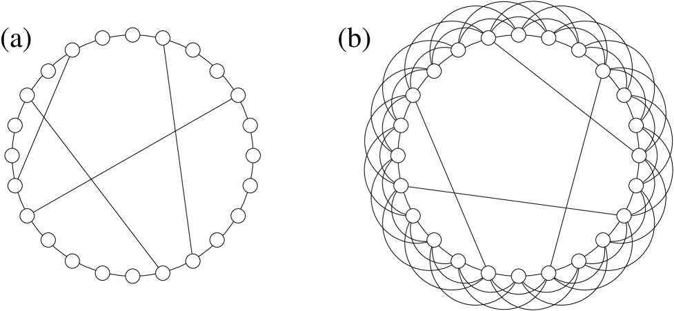
Both of these problems can be circumvented by a slight modification of the model. In our version of the small-world model we again start with a regular one-dimensional lattice, but now instead of rewiring each bond with probability $\phi$, we add shortcuts between pairs of vertices chosen uniformly at random but we do not remove any bonds from the regular lattice. We also explicitly allow there to be more than one bond between any two vertices, or a bond which connects a vertex to itself. In order to preserve compatibility with the results of Watts and Strogatz and others, we add with probability $\phi$ one shortcut for each bond on the original lattice, so that there are again $\phi L$ shortcuts on average. The average coordination number is $z=2(1+\phi)$. This model is equivalent to the Watts–Strogatz model for small $\phi$, whilst being better behaved when $\phi$ becomes comparable to 1. Fig. 1(a) shows one realization of our model for $L=24$.

Real social networks usually have average coordination numbers $z$ significantly higher than $2$, and we can arrange for higher $z$ in our model in a number of ways. Watts and Strogatz[3] proposed adding bonds to next-nearest or further neighbors on the underlying one-dimensional lattice up to some fixed range which we will call $k$[5]. In our variation on the model we can also start with such a lattice and then add shortcuts to it. The mean number of shortcuts is then $\phi kL$ and the average coordination number is $z=2k(1+\phi)$. Fig. 1(b) shows a realization of this model for $k=3$.

FIG. 2.: (a) An example of a $k=1$ small-world graph with an underlying lattice of dimension $d=2$. (b) The pattern of bonds around a vertex on the $d=2$ lattice for $k=3$.

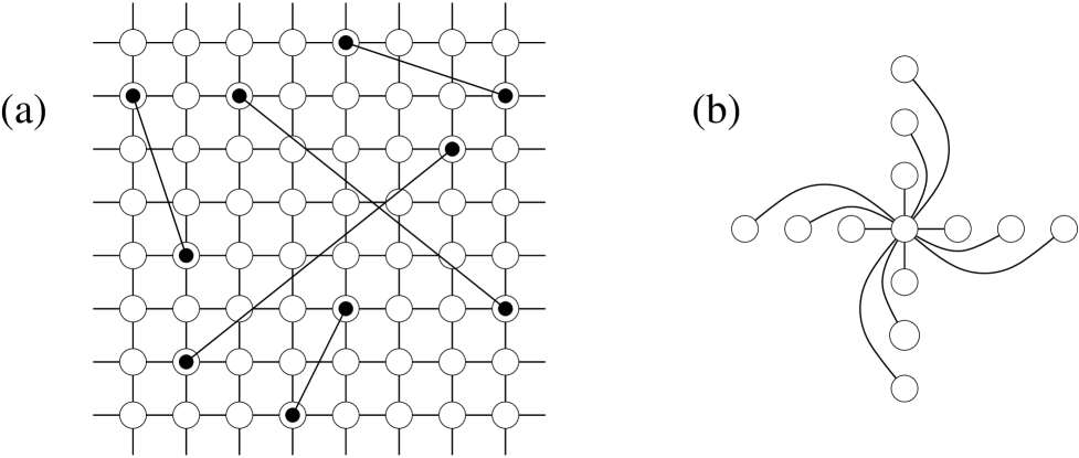
Another way of increasing the coordination number, suggested first by Watts[6, 7], is to use an underlying lattice for the model with dimension greater than one. In this paper we will consider networks based on square and (hyper)cubic lattices in $d$ dimensions. We take a lattice of linear dimension $L$, with $L^{d}$ vertices, nearest-neighbor bonds and periodic boundary conditions, and add shortcuts between randomly chosen pairs of vertices. Such a graph has $\phi dL^{d}$ shortcuts and an average coordination number $z=2d(1+\phi)$. An example is shown in Fig. 2(a) for $d=2$. We can also add bonds between next-nearest or further neighbors to such a lattice. The most straightforward generalization of the one-dimensional case is to add bonds along the principal axes of the lattice up to some fixed range $k$, as shown in Fig. 2(b) for $k=3$. Graphs of this type have $\phi kdL^{d}$ shortcuts on average and a mean coordination number of $z=2kd(1+\phi)$.

Our main interest in this paper is with the properties of the small-world model for small values of the shortcut probability $\phi$. Watts and Strogatz[3] found that the model displays many of the characteristics of true random graphs even for $\phi\ll 1$, and it seems to be in this regime that the model’s properties are most like those of real-world social networks.

III Length-scales in small-world graphs

A fundamental observable property of interest on small-world lattices is the shortest path between two vertices—the number of degrees of separation—measured as the number of bonds traversed to get from one vertex to another, averaged over all pairs of vertices and over all realizations of the randomness in the model. We denote this quantity $\ell$. On ordinary regular lattices $\ell$ scales linearly with the lattice size $L$. On the underlying lattices used in the models described here for instance, it is equal to $\frac{1}{4}dL/k$. On true random graphs, in which the probability of connection between any two vertices is the same, $\ell$ is proportional to $\log N/\log z$, where $N$ is the number of vertices on the graph[2]. The small-world model interpolates between these extremes, showing linear scaling $\ell\sim L$ for small $\phi$, or on systems small enough that there are very few shortcuts, and logarithmic scaling $\ell\sim\log N=d\log L$ when $\phi$ or $L$ is large enough. In this section and the following one we study the nature of the cross-over between these two regimes, which we refer to as “large-world” and “small-world” regimes respectively. For simplicity we will work mostly with the case $k=1$, although we will quote results for $k>1$ where they are of interest.

When $k=1$ the small-world model has only one independent parameter—the probability $\phi$—and hence can have only one non-trivial length-scale other than the lattice constant of the underlying lattice. This length-scale, which we will denote $\xi$, can be defined in a number of different ways, all definitions being necessarily proportional to one another. One simple way is to define $\xi$ to be the typical distance between the ends of shortcuts on the lattice. In a one-dimensional system with $k=1$, for example, there are on average $\phi L$ shortcuts and therefore $2\phi L$ ends of shortcuts. Since the lattice has $L$ vertices, the average distance between ends of shortcuts is $L/(2\phi L)=1/(2\phi)$. In fact, it is more convenient for our purposes to define $\xi$ without the factor of $2$ in the denominator, so that $\xi=1/\phi$, or for general $d$

$$\xi={1\over(\phi d)^{1/d}}.$$ (1)

For $k>1$ the appropriate generalization is[8]

$$\xi={1\over(\phi kd)^{1/d}}.$$ (2)

As we see, $\xi$ diverges as $\phi\to 0$ according to[9]

$$\xi\sim\phi^{-\tau},$$ (3)

where the exponent $\tau$ is

$$\tau={1\over d}.$$ (4)

A number of authors have previously considered a divergence of the kind described by Eq. (3) with $\xi$ defined not as the typical distance between the ends of shortcuts, but as the system size $L$ at which the cross-over from large- to small-world scaling occurs[10, 11, 12, 13]. We will shortly argue that in fact the length-scale $\xi$ defined here is precisely equal to this cross-over length, and hence that these two divergences are the same.

The quantity $\xi$ plays a role similar to that of the correlation length in an interacting system in standard statistical physics. Its leaves the system with no length-scale other than the lattice spacing, so that at long distances we expect all spatial distributions to be scale-free. This is precisely the behavior one sees in an interacting system undergoing a continuous phase transition, and it is reasonable to regard the small-world model as having a continuous phase transition at this point. Note that the transition is a one-sided one since $\phi$ is a probability and cannot take values less than zero. In this respect the transition is similar to that seen in the one-dimensional Ising model, or in percolation on a one-dimensional lattice. The exponent $\tau$ plays the part of a critical exponent for the system, similar to the correlation length exponent $\nu$ for a thermal phase transition.

De Menezes et al.[13] have argued that the length-scale $\xi$ can only be defined in terms of the cross-over point between large- and small-world behavior, that there is no definition of $\xi$ which can be made consistent in the limit of large system size. For this reason they argue that the transition at $\phi=0$ should be regarded as first-order rather than continuous. In fact however, the arguments of de Menezes et al. show only that one particular definition of $\xi$ is inconsistent; they show that $\xi$ cannot be consistently defined in terms of the mean vertex–vertex distance between vertices in finite regions of infinite small-world graphs. This does not prove that no definition of $\xi$ is consistent in the $L\to\infty$ limit and, as we have demonstrated here, consistent definitions do exist. Thus it seems appropriate to consider the transition at $\phi=0$ to be a continuous one.

Barthélémy and Amaral[10] have conjectured on the basis of numerical simulations that $\tau=\frac{2}{3}$ for $d=1$. As we have shown here, $\tau$ is in fact equal to $1/d$, and specifically $\tau=1$ in one dimension. We have also demonstrated this result previously using a renormalization group (RG) argument[12], and it has been confirmed by extensive numerical simulations[11, 12, 13].

The length-scale $\xi$ governs a number of other properties of small-world graphs. First, as mentioned above, it defines the point at which the average vertex–vertex distance $\ell$ crosses over from linear to logarithmic scaling with system size $L$. This statement is necessarily true, since $\xi$ is the only non-trivial length scale in the model, but we can demonstrate it explicitly by noting that the linear scaling regime is the one in which the average number of shortcuts on the lattice is small compared with unity and the logarithmic regime is the one in which it is large[6]. The cross-over occurs in the region where the average number of shortcuts is about one, or in other words when $\phi kdL^{d}=1$. Rearranging for $L$, the cross-over length is

$$L={1\over(\phi kd)^{1/d}}=\xi.$$ (5)

The length-scale $\xi$ also governs the average number $V(r)$ of neighbors of a given vertex within a neighborhood of radius $r$. The number of vertices in such a neighborhood increases as $r^{d}$ for $r\ll\xi$ while for $r\gg\xi$ the graph behaves as a random graph and the size of the neighborhood must increase exponentially with some power of $r/\xi$. To derive the specific functional form of $V(r)$ we consider a small-world graph in the limit of infinite $L$. Let $a(r)$ be the surface area of a “sphere” of radius $r$ on the underlying lattice of the model, i.e., it is the number of points which are exactly $r$ steps away from any vertex. (For $k=1$, $a(r)=2^{d}r^{d-1}/\Gamma(d)$ when $r\gg 1$.) The volume within a neighborhood of radius $r$ in an infinite system is the sum of $a(r)$ over $r$, plus a contribution of $V(r-r^{\prime})$ for every shortcut encountered at a distance $r^{\prime}$, of which there are on average $2\xi^{-d}a(r^{\prime})$. Thus $V(r)$ is in general the solution of the equation

$$V(r)=\sum_{r^{\prime}=0}^{r}a(r^{\prime})[1+2\xi^{-d}V(r-r^{\prime})].$$ (6)

In one dimension with $k=1$, for example, $a(r)=2$ for all $r$ and, approximating the sum with an integral and then differentiating with respect to $r$, we get

$${{\rm d}V\over{\rm d}r}=2[1+2V(r)/\xi],$$ (7)

which has the solution

$$V(r)=\mbox{$\frac{1}{2}$}\xi({\rm e}^{4r/\xi}-1).$$ (8)

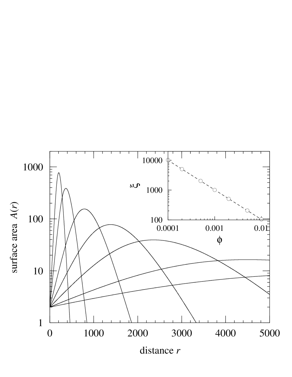
Note that for $r\ll\xi$ this scales as $r$, independent of $\xi$, and for $r\gg\xi$ it grows exponentially, as expected. Eq. (8) also implies that the surface area of a sphere of radius $r$ on the graph, which is the derivative of $V(r)$, should be

$$A(r)=2{\rm e}^{4r/\xi}.$$ (9)

These results are easily checked numerically and give us a simple independent measurement of $\xi$ which we can use to confirm our earlier arguments. In Fig. 3 we show curves of $A(r)$ from computer simulations of systems with $\phi=0.01$ for values of $L$ equal to powers of two from $128$ up to $131\,072$ (solid lines). The dotted line is Eq. (9) with $\xi$ taken from Eq. (1). The convergence of the simulation results to the predicted exponential form as the system size grows confirms our contention that $\xi$ is well-defined in the limit of large $L$. Fig. 4 shows $A(r)$ for $L=100\,000$ for various values of $\phi$. Eq. (9) implies that the slope of the lines in the limit of small $r$ is $4/\xi$. In the inset we show the values of $\xi$ extracted from fits to the slope as a function of $\phi$ on logarithmic scales, and a straight-line fit to these points gives us an estimate of $\tau=0.99\pm 0.01$ for the exponent governing the transition at $\phi=0$ (Eq. (3)). This is in good agreement with our theoretical prediction that $\tau=1$.

FIG. 3.: The mean surface area $A(r)$ of a neighborhood of radius $r$ on a $d=1$ small-world graph with $\phi=0.01$ for $L=128\ldots 131\,072$ (solid lines). The measurements are averaged over $1000$ realizations of the system each. The dotted line is the theoretical result for $L=\infty$, Eq. (9).

FIG. 4.: The mean surface area $A(r)$ of a neighborhood of radius $r$ on a $d=1$ small-world graph with $L=100\,000$ for $\phi=10^{-4}\ldots 10^{-2}$. The measurements are averaged over $1000$ realizations of the system each. Inset: the value of $\xi$ extracted from the curves in the main figure, as a function of $\phi$. The gradient of the line gives the value of the exponent $\tau$, which is found by a least squares fit (the dotted line) to be $0.99\pm 0.01$.

IV Scaling in small-world graphs

Given the existence of the single non-trivial length-scale $\xi$ for the small-world model, we can also say how the mean vertex–vertex distance $\ell$ should scale with system size and other parameters near the phase transition. In this regime the dimensionless quantity $\ell/L$ can be a function only of the dimensionless quantity $L/\xi$, since no other dimensionless combinations of variables exist. Thus we can write

$$\ell=Lf(L/\xi),$$ (10)

where $f(x)$ is an unknown but universal scaling function. A scaling form similar to this was suggested previously by Barthélémy and Amaral[10] on empirical grounds. Substituting from Eq. (1), we then get for the $k=1$ case

$$\ell=Lf(\phi^{1/d}L).$$ (11)

(We have absorbed a factor of $d^{1/d}$ into the definition of $f(x)$ here to make it consistent with the definition we used in Ref. [12].) The usefulness of this equation derives from the fact that the function $f(x)$ contains no dependence on $\phi$ or $L$ other than the explicit dependence introduced through its argument. Its functional form can however change with dimension $d$ and indeed it does. In order to obey the known asymptotic forms of $\ell$ for large and small systems, the scaling function $f(x)$ must satisfy

$$f(x)\sim{\log x\over x}\qquad\mbox{as $x\to\infty$},$$ (12)

and

$$f(x)\to\mbox{$\frac{1}{4}$}d\qquad\mbox{as $x\to 0$}.$$ (13)

When $k>1$, $\ell$ tends to $\frac{1}{4}dL/k$ for small values of $L$ and $\xi$ is given by Eq. (2), so the appropriate generalization of the scaling form is

$$\ell={L\over k}f\bigl{(}(\phi k)^{1/d}L\bigr{)},$$ (14)

with $f(x)$ taking the same limiting forms (12) and (13). Previously we derived this scaling form in a more rigorous way using an RG argument[12].

We can again test these results numerically by measuring $\ell$ on small-world graphs for various values of $\phi$, $k$ and $L$. Eq. (14) implies that if we plot the results on a graph of $\ell k/L$ against $(\phi k)^{1/d}L$, they should collapse onto a single curve for any given dimension $d$. In Fig. 5 we have done this for systems based on underlying lattices with $d=1$ for a range of values of $\phi$ and $L$, for $k=1$ and $5$. As the figure shows, the collapse is excellent. In the inset we show results for $d=2$ with $k=1$, which also collapse nicely onto a single curve. The lower limits of the scaling functions in each case are in good agreement with our theoretical predictions of $\frac{1}{4}$ for $d=1$ and $\frac{1}{2}$ for $d=2$.

FIG. 5.: Data collapse for numerical measurements of the mean vertex–vertex distance on small-world graphs with $d=1$. Circles and squares are results for $k=1$ and $k=5$ respectively for values of $L$ between $128$ and $32\,768$ and values of $\phi$ between $1\times 10^{-6}$ and $3\times 10^{-2}$. Each point is averaged over 1000 realizations of the randomness. In all cases the errors on the points are smaller than the points themselves. The dashed line is the second-order series approximation with exact coefficients given in Eq. (18), while the dot-dashed line is the fifth-order approximation using numerical results for the last three coefficients. The solid line is the third-order Padé approximant, Eqs. (21) and (26). Inset: data collapse for two-dimensional systems with $k=1$ for values of $L$ from 64 to $1024$ and $\phi$ from $3\times 10^{-6}$ up to $1\times 10^{-3}$.

We are not able to solve exactly for the form of the scaling function $f(x)$, but we can express it as a series expansion in powers of $\phi$ as follows. Since the scaling function is universal and has no implicit dependence on $k$, it is adequate to calculate it for the case $k=1$; its form is the same for all other values of $k$. For $k=1$ the probability of having exactly $m$ shortcuts on the graph is

$$P_{m}=\biggl{(}{dL^{d}\atop m}\biggr{)}\,\phi^{m}(1-\phi)^{dL^{d}-m}.$$ (15)

Let $\ell_{m}$ be the mean vertex–vertex distance on a graph with $m$ shortcuts in the limit of large $L$, averaged over all such graphs. Then the mean vertex–vertex distance averaged over all graphs regardless of the number of shortcuts is

$$\ell=\sum_{m=0}^{dL^{d}}P_{m}\ell_{m}.$$ (16)

Note that in order to calculate $\ell$ up to order $\phi^{m}$ we only need to know the behavior of the model when it has $m$ or fewer shortcuts. For the $d=1$ case the values of the $\ell_{m}$ have been calculated up to $m=2$ by Strang and Eriksson[14] and are given in Table I. Substituting these into Eq. (16) and collecting terms in $\phi$, we then find that

$${\ell\over L}=\mbox{$\frac{1}{4}-\frac{1}{24}\phi L+\frac{11}{1440}\phi^{2}L^{2}-\frac{11}{1440}\phi^{2}L+{\rm O}(\phi^{3})$}.$$ (17)

The term in $\phi^{2}L$ can be dropped when $L$ is large or $\phi$ small, since it is negligible by comparison with at least one of the terms before it. Thus the scaling function is

$$f(x)=\mbox{$\frac{1}{4}-\frac{1}{24}x+\frac{11}{1440}x^{2}+{\rm O}(x^{3})$}.$$ (18)

This form is shown as the dotted line in Fig. 5 and agrees well with the numerical calculations for small values of the scaling variable $x$, but deviates badly for large values.

	$m$	$\ell_{m}/L$
	0	$1/4$
	1	$5/24$
	2	$131/720$
	3	$0.1549\pm 0.0003$
	4	$0.1365\pm 0.0003$
	5	$0.1232\pm 0.0003$

TABLE I.: Average vertex–vertex distances per vertex $\ell_{m}/L$ on $d=1$ small-world graphs with exactly $m$ shortcuts and $k=1$. Values up to $m=2$ are the exact results of Strang and Eriksson[14]. Values for $m=3\ldots 5$ are our numerical results.

Calculating the exact values of the quantities $\ell_{m}$ for higher orders is an arduous task and probably does not justify the effort involved. However, we have calculated the values of the $\ell_{m}$ numerically up to $m=5$ by evaluating the average vertex–vertex distance $\ell$ on graphs which are constrained to have exactly 3, 4 or 5 shortcuts. Performing a Taylor expansion of $\ell/L$ about $L=\infty$, we get

$${\ell\over L}={\ell_{m}\over L}\Bigl{[}1+{c\over L}+{\rm O}\bigl{(}L^{-2}\bigr{)}\Bigr{]},$$ (19)

where $c$ is a constant. Thus we can estimate $\ell_{m}/L$ from the vertical-axis intercept of a plot of $\ell/L$ against $L^{-1}$ for large $L$. The results are shown in Table I. Calculating higher orders still would be straightforward.

Using these values we have evaluated the scaling function $f(x)$ up to fifth order in $x$; the result is shown as the dot–dashed line in Fig. 5. As we can see the range over which it matches the numerical results is greater than before, but not by much, indicating that the series expansion converges only slowly as extra terms are added. It appears therefore that series expansion would be a poor way of calculating $f(x)$ over the entire range of interest.

A much better result can be obtained by using our series expansion coefficients to define a Padé approximant to $f(x)$[15, 16]. Since we know that $f(x)$ tends to a constant $f(0)=\frac{1}{4}d$ for small $x$ and falls off approximately as $1/x$ for large $x$, the appropriate Padé approximants to use are odd-order approximants where the approximant of order $2n+1$ ($n$ integer) has the form

$$f(x)=f(0){A_{n}(x)\over B_{n+1}(x)},$$ (20)

where $A_{n}(x)$ and $B_{n}(x)$ are polynomials in $x$ of degree $n$ with constant term equal to 1. For example, to third order we should use the approximant

$$f(x)=f(0){1+a_{1}x\over 1+b_{1}x+b_{2}x^{2}}.$$ (21)

Expanding about $x=0$ this gives

$${f(x)\over f(0)} = 1+(a_{1}-b_{1})x+(b_{1}^{2}-a_{1}b_{1}-b_{2})x^{2}$$ (23)

$$+[(a_{1}-b_{1})(b_{1}^{2}-b_{2})+b_{1}b_{2}]x^{3}+{\rm O}(x^{4}).$$

Equating coefficients order by order in $x$ and solving for the $a$’s and $b$’s, we find that

$$a_{1} = 1.825\pm 0.075,$$ (25)

$$b_{1} = 1.991\pm 0.075,$$ (26)

$$b_{2} = 0.301\pm 0.012.$$ (27)

Substituting these back into (21) and using the known value of $f(0)$ then gives us our approximation to $f(x)$. This approximation is plotted as the solid line in Fig. 5 and, as the figure shows, is an excellent guide to the value of $f(x)$ over a large range of $x$. In theory it should be possible to calculate the fifth-order Padé approximant using the numerical results in Table I, although we have not done this here. Substituting $f(x)$ back into the scaling form, Eq. (14), we can also use the Padé approximant to predict the value of the mean vertex–vertex distance for any values of $\phi$, $k$ and $L$ within the scaling regime. We will make use of this result in the next section to calculate the effective dimension of small-world graphs.

V Effective dimension

The calculation of the volumes and surface areas of neighborhoods of vertices on small-world graphs in Section III leads us naturally to the consideration of the dimension of these systems. On a regular lattice of dimension $D$, the volume $V(r)$ of a neighborhood of radius $r$ increases in proportion to $r^{D}$, and hence one can calculate $D$ from[17]

$$D={{\rm d}\log V\over{\rm d}\log r}={rA(r)\over V(r)},$$ (28)

where $A(r)$ is the surface area of the neighborhood, as previously. We can use the same expression to calculate the effective dimension of our small-world graphs. Thus in the case of an underlying lattice of dimension $d=1$, the effective dimension of the graph is

$$D={4r\over\xi}\,{{\rm e}^{4r/\xi}\over{\rm e}^{4r/\xi}-1},$$ (29)

where we have made use of Eqs. (8) and (9). For $r\ll\xi$ this tends to one, as we would expect, and for $r\gg\xi$ it tends to $4r/\xi$, increasing linearly with the radius of the neighborhood. Thus the effective dimension of a small-world graph depends on the length-scale on which we look at it, in a way reminiscent of the behavior of multifractals[18, 19]. This result will become important in Section VI when we consider site percolation on small-world graphs.

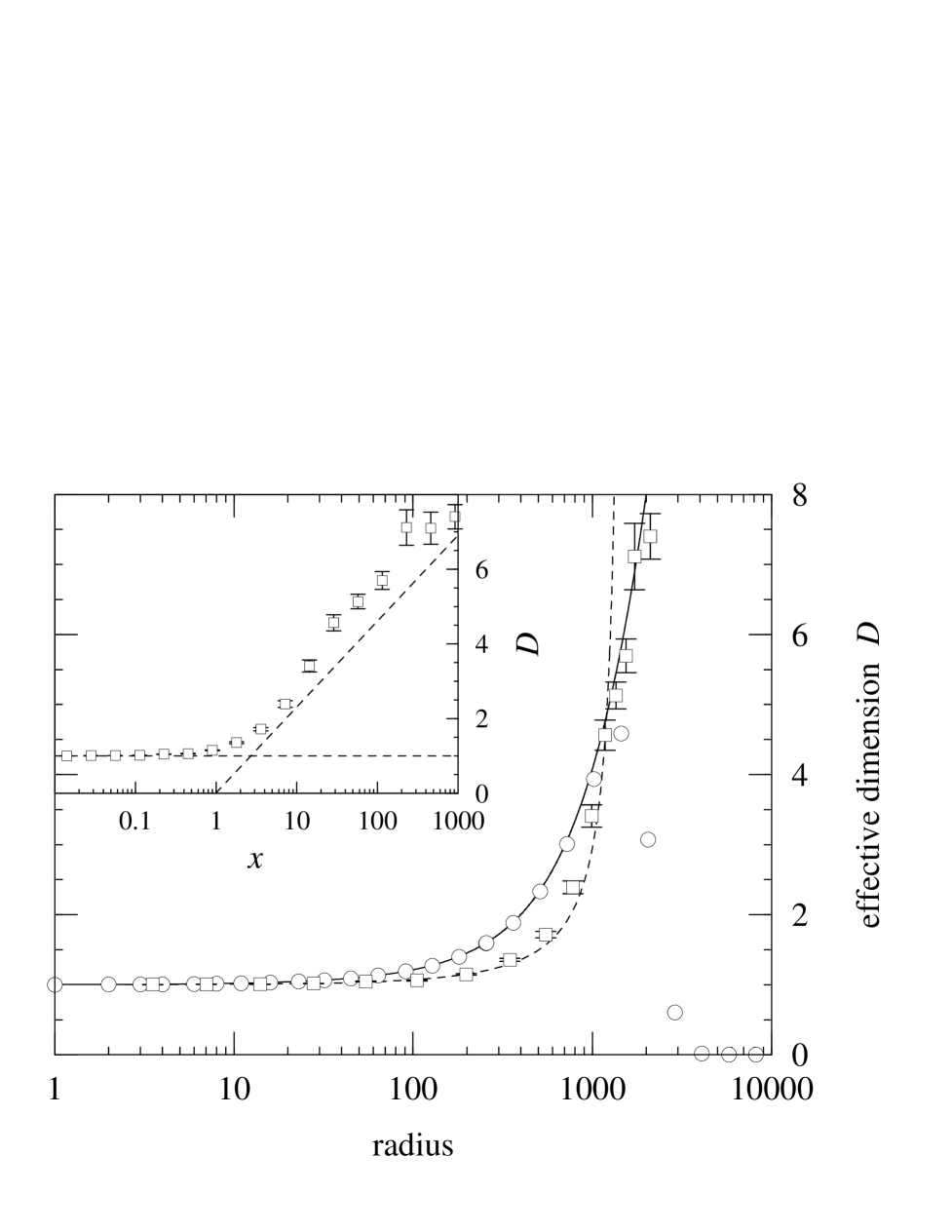
In Fig. 6 we show the effective dimension of neighborhoods on a large graph measured in numerical simulations (circles), along with the analytic result, Eq. (29) (solid line). As we can see from the figure, the numerical and analytic results are in good agreement for small radii $r$, but the numerical results fall off sharply for larger $r$. The reason for this is that Eq. (28) breaks down as $V(r)$ approaches the volume of the entire system; $V(r)$ must tend to $L^{d}$ in this limit and hence the derivative in (28) tends to zero. The same effect is also seen if one tries to use Eq. (28) on ordinary regular lattices of finite size. To characterize the dimension of an entire system therefore, we use another measure of $D$ as follows.

FIG. 6.: Effective dimension $D$ of small-world graphs. The circles are results for $D$ from numerical calculations on an $L=1\,000\,000$ system with $d=1$, $k=1$ and $\phi=10^{-3}$ using Eq. (28). The errors on the points are in all cases smaller than the points themselves. The solid line is Eq. (29). The squares are calculated from Eq. (31) by numerical differentiation of simulation results for the scaling function $f(x)$ of one-dimensional systems. The dotted line is Eq. (31) evaluated using the third-order Padé approximant to the scaling function derived in Section IV. Inset: effective dimension from Eq. (31) plotted as a function of the scaling variable $x$. The dotted lines represent the asymptotic forms for large and small $x$ discussed in the text.

On a regular lattice of finite linear size $\ell$, the number of vertices $N$ scales as $\ell^{D}$ and hence we can calculate the dimension from

$$D={{\rm d}\log N\over{\rm d}\log\ell}.$$ (30)

We can apply the same formula to the calculation of the effective dimension of small-world graphs putting $N=L^{d}$, although, since we don’t have an analytic solution for $\ell$, we cannot derive an analytic solution for $D$ in this case. On the other hand, if we are in the scaling regime described in Section IV—the regime in which $\xi\gg 1$—then Eq. (14) applies, along with the limiting forms, Eqs. (12) and (13). Substituting into (30), this gives us

$${1\over D}={{\rm d}\log\ell\over{\rm d}\log L^{d}}={1\over d}\biggl{[}1+{{\rm d}\log f(x)\over{\rm d}\log x}\biggr{]},$$ (31)

where $x=(\phi k)^{1/d}L\propto L/\xi$. In other words $D$ is a universal function of the scaling variable $x$. We know that $f(x)$ tends to a constant for small $x$ (i.e., $\xi\gg L$), so that $D=d$ in this limit, as we would expect. For large $x$ (i.e., $\xi\ll L$), Eq. (12) applies. Substituting into (31) this gives us $D=d\log x$. In the inset of Fig. 6 we show $D$ from numerical calculations as a function of $x$ in one-dimensional systems of a variety of sizes, along with the expected asymptotic forms, which it follows reasonably closely. In the main figure we also show this second measure of $D$ (squares with error bars) as a function of the system radius $\ell$ (with which it should scale linearly for large $\ell$, since $\ell\sim\log x$ for large $x$). As the figure shows, the two measures of effective dimension agree reasonably well. The numerical errors on the first measure, Eq. (28) are much smaller than those on the second, Eq. (30) (which is quite hard to calculate numerically), but the second measure is clearly preferable as a measure of the dimension of the entire system, since the first fails badly when $r$ approaches $\ell$. We also show the value of our second measure of dimension calculated using the Padé approximant to $f(x)$ derived in Section IV (dotted line in the main figure). This agrees well with the numerical evaluation for radii up to about $1000$ and has significantly smaller statistical error, but overestimates $D$ somewhat beyond this point because of inaccuracies in the approximation; the Padé approximant scales as $1/x$ for large values of $x$ rather than $\log x/x$, which means that $D$ will scale as $x$ rather than $\log x$ for large $x$.

VI Percolation

In the previous sections of this paper we have examined statistical properties of small-world graphs such as typical length-scales, vertex–vertex distances, scaling of volumes and areas, and effective dimension of graphs. These are essentially static properties of the networks; to the extent that small-world graphs mimic social networks, these properties tell us about the static structure of those networks. However, social science also deals with dynamic processes going on within social networks, such as the spread of ideas, information, or diseases. This leads us to the consideration of dynamical models defined on small-world graphs. A small amount of research has already been conducted in this area. Watts[6, 7], for instance, has considered the properties of a number of simple dynamical systems defined on small-world graphs, such as networks of coupled oscillators and cellular automata. Barrat and Weigt[20] have looked at the properties of the Ising model on small-world graphs and derived a solution for its partition function using the replica trick. Monasson[21] looked at the spectral properties of the Laplacian operator on small-world graphs, which tells us about the time evolution of a diffusive field on the graph. There is also a moderate body of work in the mathematical and social sciences which, although not directly addressing the small-world model, deals with general issues of information propagation in networks, such as the adoption of innovations[22, 23, 24, 25], human epidemiology[26, 27, 28], and the flow of data on the Internet[29, 30].

In this section we discuss the modeling of information or disease propagation specifically on small-world graphs. Suppose for example that the vertices of a small-world graph represent individuals and the bonds between them represent physical contact by which a disease can be spread. The spread of ideas can be similarly modeled; the bonds then represent information connections between individuals which could include letters, telephone calls, or email, as well as physical contacts. The simplest model for the spread of disease is to have the disease spread between neighbors on the graph at a uniform rate, starting from some initial carrier individual. From the results of Section IV we already know what this will look like. If for example we wish to know how many people in total have contracted a disease, that number is just equal to the number $V(r)$ within some radius $r$ of the initial carrier, where $r$ increases linearly with time. (We assume that no individual can catch the disease twice, which is the case with most common diseases.) Thus, Eq. (8) tells us that, for a $d=1$ small-world graph, the number of individuals who have had a particular disease increases exponentially, with a time-constant governed by the typical length-scale $\xi$ of the graph. Since all real-world social networks have a finite number of vertices $N$, this exponential growth is expected to saturate when $V(r)$ reaches $N=L^{d}$. This is not a particularly startling result; the usual model for the spread of epidemics is the logistic growth model, which shows initial exponential spread followed by saturation.

For a disease like influenza, which spreads fast but is self-limiting, the number of people who are ill at any one time should be roughly proportional to the area $A(r)$ of the neighborhood surrounding the initial carrier, with $r$ again increasing linearly in time. This implies that the epidemic should have a single humped form with time, like the curves of $A(r)$ plotted in Fig. 4. Note that the vertical axis in this figure is logarithmic; on linear axes the curves are bell-shaped rather than quadratic. In the context of the spread of information or ideas, similar behavior might be seen in the development of fads. By a fad we mean an idea which is catchy and therefore spreads fast, but which people tire of quickly. Fashions, jokes, toys, or buzzwords might be expected to show popularity profiles over time similar to the curves in Fig. 4.

However, for most real diseases (or fads) this is not a very good model of how they spread. For real diseases it is commonly the case that only a certain fraction $p$ of the population is susceptible to the disease. This can be mimicked in our model by placing a two-state variable on each vertex which denotes whether the individual at that vertex is susceptible. The disease then spreads only within the local “cluster” of connected susceptible vertices surrounding the initial carrier. One question which we can answer with such a model is how high the density $p$ of susceptible individuals can be before the largest connected cluster covers a significant fraction of the entire network and an epidemic ensues.

Mathematically, this is precisely the problem of site percolation on a social network, at least in the case where the susceptible individuals are randomly distributed over the vertices. To the extent that small-world graphs mimic social networks, therefore, it is interesting to look at the percolation problem. The transition corresponds to the point on a regular lattice at which a percolating cluster forms whose size increases with the size $L$ of the lattice for arbitrarily large $L$[31]. On random graphs there is a similar transition, marked by the formation of a so-called “giant component” of connected vertices[32]. On small-world graphs we can calculate approximately the percolation probability $p=p_{c}$ at which the transition takes place as follows.

Consider a $d=1$ small-world graph of the kind pictured in Fig. 1. For the moment let us ignore the shortcut bonds and consider the percolation properties just of the underlying regular lattice. If we color in a fraction $p$ of the sites on this underlying lattice, the occupied sites will form a number of connected clusters. In order for two adjacent parts of the lattice not to be connected, we must have a series of at least $k$ consecutive unoccupied sites between them. The number $n$ of such series can be calculated as follows. The probability that we have a series of $k$ unoccupied sites starting at a particular site, followed by an occupied one is $p(1-p)^{k}$. Once we have such a series, the states of the next $k$ sites are fixed and so it is not possible to have another such series for $k$ steps. Thus the number $n$ is given by

$$n=p(1-p)^{k}(L-kn).$$ (32)

Rearranging for $n$ we get

$$n=L\,{p(1-p)^{k}\over 1+kp(1-p)^{k}}.$$ (33)

For this one-dimensional system, the percolation transition occurs when we have just one break in the chain, i.e., when $n=1$. This gives us a $k$th order equation for $p_{c}$ which is in general not exactly soluble, but we can find its roots numerically if we wish.

Now consider what happens when we introduce shortcuts into the graph. The number of breaks $n$, Eq. (33), is also the number of connected clusters of occupied sites on the underlying lattice. Let us for the moment suppose that the size of each cluster can be approximated by the average cluster size. A number $\phi kL$ of shortcuts are now added to the graph between pairs of vertices chosen uniformly at random. A fraction $p^{2}$ of these will connect two occupied sites and therefore can connect together two clusters of occupied sites. The problem of when the percolation transition occurs is then precisely that of the formation of a giant component on an ordinary random graph with $n$ vertices. It is known that such a component forms when the mean coordination number of the random graph is one[32], or alternatively, when the number of bonds on the graph is a half the number of vertices. In other words, the transition probability $p_{c}$ must satisfy

$$p_{c}^{2}\phi kL=\mbox{$\frac{1}{2}$}L\,{p_{c}(1-p_{c})^{k}\over 1+kp_{c}(1-p_{c})^{k}},$$ (34)

or

$$\phi={(1-p_{c})^{k}\over 2kp_{c}[1+kp_{c}(1-p_{c})^{k}]}.$$ (35)

We have checked this result against numerical calculations. In order to find the value of $p_{c}$ numerically, we employ a tree-based invasion algorithm similar to the invaded cluster algorithm used to find the percolation point in Ising systems[33, 34]. This algorithm can calculate the entire curve of average cluster size versus $p$ in time which scales as $L\log L$[35]. We define $p_{c}$ to be the point at which the average cluster size divided by $L$ rises above a certain threshold. For systems of infinite size the transition is instantaneous and hence the choice of threshold makes no difference to $p_{c}$, except that $p_{c}$ can never take a value lower than the threshold itself, since even in a fully connected graph the average cluster size per vertex can be no greater than the fraction $p_{c}$ of occupied vertices. Thus it makes sense to choose the threshold as low as possible. In real calculations, however, we cannot use an infinitesimal threshold because of finite size effects. For the systems studied here we have found that a threshold of $0.2$ works well.

FIG. 7.: Numerical results for the percolation threshold on $L=10\,000$ small-world graphs with $k=1$ (circles), 2 (squares), and 5 (triangles) as a function of the shortcut density $\phi$. The solid lines are the analytic approximation to the same quantity, Eq. (35).

Fig. 7 shows the critical probability $p_{c}$ for systems of size $L=10\,000$ for a range of values of $\phi$ for $k=1$, 2 and 5. The points are the numerical results and the solid lines are Eq. (35). As the figure shows the agreement between simulation and theory is good although there are some differences. As $\phi$ approaches one and the value of $p_{c}$ drops, the two fail to agree because, as mentioned above, $p_{c}$ cannot take a value lower than the threshold used in its calculation, which was $0.2$ in this case. The results also fail to agree for very low values of $\phi$ where $p_{c}$ becomes large. This is because Eq. (33) is not a correct expression for the number of clusters on the underlying lattice when $n<1$. This is clear since when there are no breaks in the sequence of connected vertices around the ring it is not also true that there are no connected clusters. In fact there is still one cluster; the equality between number of breaks and number of clusters breaks down at $n=1$. The value of $p$ at which this happens is given by putting $n=1$ in Eq. (32). Since $p$ is close to one at this point its value is well approximated by

$$p\simeq 1-L^{-1/k},$$ (36)

and this is the value at which the curves in Fig. 7 should roll off at low $\phi$. For $k=5$ for example, for which the roll-off is most pronounced, this expression gives a value of $p\simeq 0.8$, which agrees reasonably well with what we see in the figure.

There is also an overall tendency in Fig. 7 for our analytic expression to overestimate the value of $p_{c}$ slightly. This we put down to the approximation we made in the derivation of Eq. (35) that all clusters of vertices on the underlying lattice can be assumed to have the size of the average cluster. In actual fact, some clusters will be smaller than the average and some larger. Since the shortcuts will connect to clusters with probability proportional to the cluster size, we can expect percolation to set in within the subset of larger-than-average clusters before it would set in if all clusters had the average size. This makes the true value of $p_{c}$ slightly lower than that given by Eq. (35). In general however, the equation gives a good guide to the behavior of the system.

We have also examined numerically the behavior of the mean cluster radius $\rho$ for percolation on small-world graphs. The radius of a cluster is defined as the average distance between vertices within the cluster, along the edges of the graph within the cluster. This quantity is small for small values of the percolation probability $p$ and increases with $p$ as the clusters grow larger. When we reach percolation and a giant component forms it reaches a maximum value and then drops as $p$ increases further. The drop happens because the percolating cluster is most filamentary when percolation has only just set in and so paths between vertices are at their longest. With further increases in $p$ the cluster becomes more highly connected and the average shortest path between two vertices decreases.

FIG. 8.: Average cluster radius $\rho$ as a function of the percolation probability $p$ for site percolation on small-world graphs with $k=1$, $\phi=0.1$ and $L$ equal to a power from $512$ up to $16\,384$ (circles, squares, diamonds, upward-pointing triangles, left-pointing triangles and downward-pointing triangles respectively). Each set of points is averaged over 100 realizations of the corresponding graph. Inset: the same data collapsed according to Eq. (37) with $\nu=0.59$, $\gamma=1.3$ and $p_{c}=0.74$.

By analogy with percolation on regular lattices we might expect the average cluster radius for a given value of $\phi$ to satisfy the scaling form[31]

$$\rho=\ell^{\gamma/\nu}\widetilde{\rho}\bigl{(}(p-p_{c})\ell^{1/\nu}\bigr{)},$$ (37)

where $\widetilde{\rho}(x)$ is a universal scaling function, $\ell$ is the radius of the entire system and $\gamma$ and $\nu$ are critical exponents. In fact this scaling form is not precisely obeyed by the current system because the exponents $\nu$ and $\gamma$ depend in general on the dimension of the lattice. As we showed in Section V, the dimension $D$ of a small-world graph depends on the length-scale on which you look at it. Thus the value of $D$ “felt” by a cluster of radius $\rho$ will vary with $\rho$, implying that $\nu$ and $\gamma$ will vary both with the percolation probability and with the system size. If we restrict ourselves to a region sufficiently close to the percolation threshold, and to a sufficiently small range of values of $\ell$, then Eq. (37) should be approximately correct.

FIG. 9.: Best fit values of $p_{c}$ as a function of $1/\nu$. Inset: the values are calculated from the vertical-axis intercept of a plot of the position $p_{0}$ of the peak of $\rho$ against $\ell^{-1/\nu}$ (see Eq. (38)).

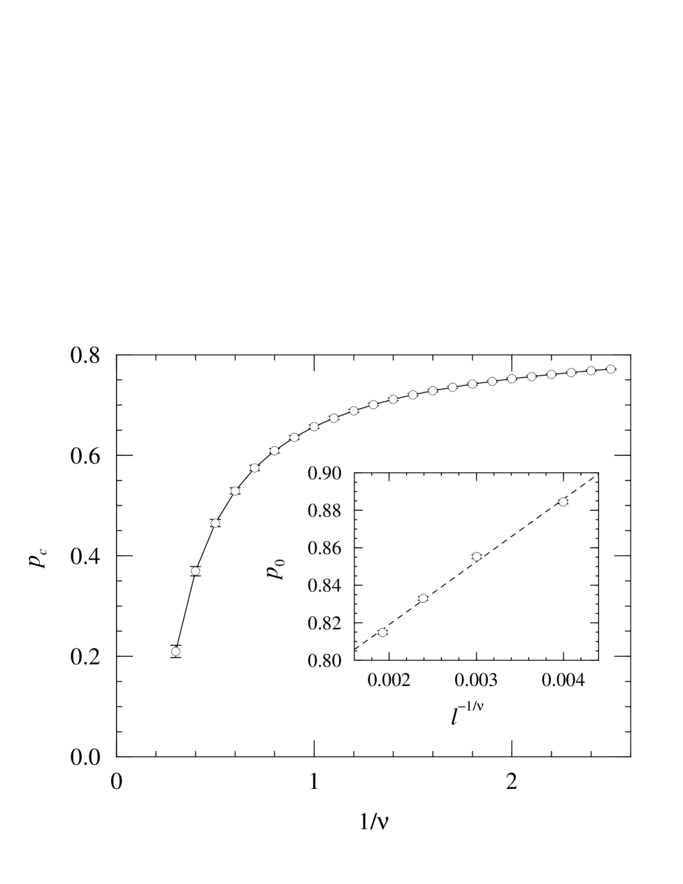
In Fig. 8 we show numerical data for $\rho$ for small-world graphs with $k=1$, $\phi=0.1$ and $L$ equal to a power of two from 512 up to $16\,384$. As we can see, the data show the expected peaked form, with the peak in the region of $p=0.8$, close to the expected position of the percolation transition. In order to perform a scaling collapse of these data we need first to extract a suitable value of $p_{c}$. We can do this by performing a fit to the positions of the peaks in $\rho$[36]. Since the scaling function $\widetilde{\rho}(x)$ is (approximately) universal, the positions of these peaks all occur at the same value of the scaling variable $y=(p-p_{c})\ell^{1/\nu}$. Calling this value $y_{0}$ and the corresponding percolation probability $p_{0}$, we can rearrange for $p_{0}$ as a function of $\ell$ to get

$$p_{0}=p_{c}+y_{0}\ell^{-1/\nu}.$$ (38)

Thus if we plot the measured positions $p_{0}$ as a function of $\ell^{-1/\nu}$, the vertical-axis intercept should give us the corresponding value of $p_{c}$. We have done this for a single value of $\nu$ in the inset to Fig. 9, and in the main figure we show the resulting values of $p_{c}$ as a function of $1/\nu$. If we now perform our scaling collapse, with the restriction that the values of $\nu$ and $p_{c}$ fall on this line, then the best coincidence of the curves for $\rho$ is obtained when $p_{c}=0.74$ and $\nu=0.59\pm 0.05$—see the inset to Fig. 8. The value of $\gamma$ can be found separately by requiring the heights of the peaks to match up, which gives $\gamma=1.3\pm 0.1$. The collapse is noticeably poorer when we include systems of size smaller than $L=512$, and we attribute this not merely to finite size corrections to the scaling form, but also to variation in the values of the exponents $\gamma$ and $\nu$ with the effective dimension of the percolating cluster.

The value $p_{c}=0.74$ is in respectable agreement with the value of $0.82$ from our direct numerical measurements. We note that $\nu$ is expected to tend to $\frac{1}{2}$ in the limit of an infinite-dimensional system. The value $\nu=0.59$ found here therefore confirms our contention that small-world graphs have a high effective dimension even for quite moderate values of $\phi$, and thus are in some sense close to being random graphs. (On a two-dimensional lattice by contrast $\nu=\frac{4}{3}$.)

VII Conclusions

In this paper we have studied the small-world network model of Watts and Strogatz, which mimics the behavior of networks of social interactions. Small-world graphs consist of a set of vertices joined together in a regular lattice, plus a low density of “shortcuts” which link together pairs of vertices chosen at random. We have looked at the scaling properties of small-world graphs and argued that there is only one typical length-scale present other than the fundamental lattice constant, which we denote $\xi$ and which is roughly the typical distance between the ends of shortcuts. We have shown that this length-scale governs the transition of the average vertex–vertex distance on a graph from linear to logarithmic scaling with increasing system size, as well as the rate of growth of the number of vertices in a neighborhood of fixed radius about a given point. We have also shown that the value of $\xi$ diverges on an infinite lattice as the density of shortcuts tends to zero, and therefore that the system possesses a continuous phase transition in this limit. Close to the phase transition, where $\xi$ is large, we have shown that the average vertex–vertex distance on a finite graph obeys a simple scaling form and in any given dimension is a universal function of a single scaling variable which depends on the density of shortcuts, the system size and the average coordination number of the graph. We have calculated the form of the scaling function to fifth order in the shortcut density using a series expansion and to third order using a Padé approximant. We have defined two measures of the effective dimension $D$ of small-world graphs and find that the value of $D$ depends on the scale on which you look at the graph in a manner reminiscent of the behavior of multifractals. Specifically, at length-scales shorter than $\xi$ the dimension of the graph is simply that of the underlying lattice on which it is built, and for length-scales larger than $\xi$ it increases linearly, with a characteristic constant proportional to $\xi$. The value of $D$ increases logarithmically with the number of vertices in the graph. We have checked all of these results by extensive numerical simulation of the model and in all cases we find good agreement between the analytic predictions and the simulation results.

In the last part of the paper we have looked at site percolation on small-world graphs as a model of the spread of information or disease in social networks. We have derived an approximate analytic expression for the percolation probability $p_{c}$ at which a “giant component” of connected vertices forms on the graph and shown that this agrees well with numerical simulations. We have also performed extensive numerical measurements of the typical radius of connected clusters on the graph as a function of the percolation probability and shown by performing a scaling collapse that these obey, to a reasonable approximation, the expected scaling form in the vicinity of the percolation transition. The characteristic exponent $\nu$ takes a value close to $\frac{1}{2}$, indicating that, as far as percolation is concerned, the graph’s properties are close to those of a random graph.

REFERENCES

- [1] S. Milgram, “The small world problem,” Psychol. Today 2, 60–67 (1967).
- [2] B. Bollobás, Random Graphs, Academic Press, New York (1985).
- [3] D. J. Watts and S. H. Strogatz, “Collective dynamics of ‘small-world’ networks,” Nature 393, 440–442 (1998).
- [4] In previous work the letter has been used to denote the density of random connections, rather than . We use here however, to avoid confusion with the percolation probability introduced in Section VI, which is also conventionally denoted .
- [5] Watts and Strogatz used the letter to refer to the average coordination number, but we will find it convenient to distinguish between the coordination number, which we call , and the range of the bonds. In one dimension and in general for networks based on -dimensional lattices.
- [6] D. J. Watts, The Structure and Dynamics of Small-World Systems, Ph.D. thesis, Cornell University (1997).
- [7] D. J. Watts, Small Worlds: The Dynamics of Networks Between Order and Randomness, Princeton University Press, Princeton (1999).
- [8] The exact definition of depends on how you measure lengths in the model. The definition given here is appropriate if is measured in terms of the lattice constant of the underlying lattice. It would however be reasonable to measure it in terms of the number of bonds traversed between the ends of two shortcuts. Since we are measuring lattice size in terms of the underlying lattice constant rather than number of bonds, the present definition is the more appropriate one in our case, but it would be perfectly consistent to define both and to be a factor of smaller; all the physical results would work out the same.
- [9] In a system of finite size the average distance between the ends of two shortcuts cannot be larger than , so we cannot observe this divergence once is larger than this.
- [10] M. Barthélémy and L. A. N. Amaral, “Small-world networks: Evidence for a crossover picture,” Phys. Rev. Lett. 82, 3180–3183 (1999).
- [11] A. Barrat, “Comment on ‘Small-world networks: Evidence for a crossover picture’,” submitted to Phys. Rev. Lett. Also cond-mat/9903323.
- [12] M. E. J. Newman and D. J. Watts, “Renormalization group analysis of the small-world network model,” submitted to Phys. Rev. Lett. Also cond-mat/9903357.
- [13] M. Argollo de Menezes, C. F. Moukarzel and T. J. P. Penna, “First-order transition in small-world networks,” submitted to Phys. Rev. Lett. Also cond-mat/9903426.
- [14] G. Strang and H. Eriksson, in preparation.
- [15] D. S. Gaunt and A. J. Guttmann, “Asymptotic Analysis of Coefficients,” in Phase Transitions and Critical Phenomena, Vol. 3, C. Domb and M. S. Green (eds.), Academic Press, London (1974).
- [16] We are indebted to Prof. S. H. Strogatz for suggesting the use of a Padé approximant in this context.
- [17] We use the capital letter to denote the dimension here, to distinguish it from the dimension of the underlying lattice defined in Section II.
- [18] B. B. Mandelbrot, “Intermittent turbulence in self-similar cascades: Divergence of high moments and dimension of the carrier,” J. Fluid Mech. 62, 331–358 (1974).
- [19] T. C. Halsey, M. H. Jensen, L. P. Kadanoff, I. Procaccia, and B. I. Shraiman, “Fractal measures and their singularities: The characterization of strange sets,” Phys. Rev. A 33, 1141–1151 (1986).
- [20] A. Barrat and M. Weigt, “On the properties of small-world network models,” submitted to Eur. Phys. J. B. Also cond-mat/9903411.
- [21] R. Monasson, “Diffusion, localization and dispersion relations on small-world lattices,” submitted to Eur. Phys. J. B. Also cond-mat/9903347.
- [22] E. M. Rogers, Diffusion of Innovations, Free Press, New York (1962).
- [23] J. S. Coleman, E. Katz and H. Menzel, Medical Innovation: A Diffusion Study, Bobbs–Merrill, Indianapolis (1966).
- [24] D. Strang, “Adding social structure to diffusion models,” Sociological Methods and Research 19, 324–353 (1991).
- [25] T. W. Valente, “Social network thresholds in the diffusion of innovations,” Social Networks 18, 69–89 (1996).
- [26] L. Sattenspiel and C. P. Simon, “The spread and persistence of infectious diseases in structured populations,” Math. Biosciences 90, 367–383 (1988).
- [27] M. Kretschmar and M. Morris, “Measures of concurrency in networks and the spread of infectious disease,” Math. Biosci. 133, 165–195 (1996).
- [28] I. M. Logini, Jr., “A mathematical model for predicting the geographic spread of new infectious agents,” Math. Biosci. 90, 341–366 (1988).
- [29] J. O. Kephart and S. R. White, “Directed-graph epidemiological models of computer viruses,” in Proceedings of the 1991 IEEE Computer Science Symposium on Research in Security and Privacy, IEEE Computer Society Press, Los Alamitos (1991).
- [30] J. E. Hanson and J. O. Kephart, “Combatting maelstroms in networks of communicating agents,” to appear in Proceedings of the Sixteenth National Conference on Artificial Intelligence, American Association for Artificial Intelligence, Menlo Park (1999).
- [31] D. Stauffer and A. Aharony, Introduction to Percolation Theory, 2nd edition. Taylor and Francis, London (1992).
- [32] N. Alon and J. H. Spencer, The Probabilistic Method, Wiley, New York (1992).
- [33] J. Machta, Y. S. Choi, A. Lucke, T. Schweizer, and L. V. Chayes, “Invaded cluster algorithm for equilibrium critical points,” Phys. Rev. Lett. 75, 2792–2795 (1995).
- [34] G. T. Barkema and M. E. J. Newman, “New Monte Carlo algorithms for classical spin systems,” in Monte Carlo Methods in Chemical Physics, D. Ferguson, J. I. Siepmann, and D. G. Truhlar (eds.), Wiley, New York (1999).
- [35] A naive recursive cluster-finding algorithm by contrast takes time proportional to .
- [36] M. E. J. Newman and G. T. Barkema, Monte Carlo Methods in Statistical Physics, Oxford University Press, Oxford (1999).