Active Width at a Slanted Active Boundary in Directed Percolation

Abstract

The width $W$ of the active region around an active moving wall in a directed percolation process diverges at the percolation threshold $p_{c}$ as $W\simeq A\epsilon^{-\nu_{\parallel}}\ln(\frac{\epsilon_{0}}{\epsilon})$, with $\epsilon=p_{c}-p$, $\epsilon_{0}$ a constant, and $\nu_{\parallel}=1.734$ the critical exponent of the characteristic time needed to reach the stationary state $\xi_{\parallel}\sim\epsilon^{-\nu_{\parallel}}$. The logarithmic factor arises from screening of statistically independent needle shaped sub clusters in the active region. Numerical data confirm this scaling behaviour.

I Introduction

Directed percolation (DP) has emerged as one of the generic absorbing state type dynamic processes. It describes epidemic processes, e.g., forest fires and various types of surface catalysis processes [1, 2, 3, 4, 5]. Such processes include a so-called absorbing state, typically the vacuum, from which it can not escape. The relevant tunable parameter is the propagation probability $p$. The system undergoes a phase transition from the absorbing phase at small $p$, where the stationary state is the absorbing state, into an active stationary phase at large $p$, where the system refuses to die. The scaling properties at DP dynamic phase transitions are known for almost two decades, and it’s now realized that DP critical behaviour is the generic universality class for dynamic absorbing state type processes [1].

At DP type critical points the equilibration time $\xi_{\parallel}$ diverges. It scales as $\xi_{\parallel}\sim\xi_{\perp}^{z}$ compared to the spatial correlation length $\xi_{\perp}$, with dynamic exponent $z=1.581$[6]. For example, starting from a single seed, the survival probability obeys the scaling form

$$P_{s}(\epsilon,t)=b^{-x_{s}}P_{s}(b^{1/\nu_{\perp}}\epsilon,b^{-z}t)$$ (1)

with $\epsilon=p_{c}-p$ the distance from the critical point. This leads to

$$P_{s}\sim\epsilon^{\beta}\exp(\frac{-t}{\xi_{\parallel}}),$$ (2)

with exponent $\beta=x_{s}\nu_{\perp}$. The exponential factor reflects that deep inside the absorbing phase $P_{s}$ decays exponentially in time. The equilibration time diverges at the DP critical point as $\xi_{\parallel}\sim\epsilon^{-\nu_{\parallel}}$ with $z=\nu_{\parallel}/\nu_{\perp}$. At $p_{c}$ the survival probability decays as a powerlaw, $P_{s}(t)\sim t^{-\delta}$ with $\delta=x_{s}/z=\beta/\nu_{\parallel}$.

A recent direction of research in this topic concerns the scaling properties near boundaries [7, 8, 9, 10]. Those studies address absorbing and reflective walls. The scaling properties are modified by surface type critical exponents. In particular, the survival probability for a seed near the boundary obeys the same scaling form as above, but with a new interface critical exponent $x$, and therefore a modified value for $\beta$.

In this study we discuss the scaling properties near active boundaries. Consider a stationary active vertical wall in the system. All sites in the wall are alive. The critical exponent $\beta$ is not an issue, because the system remains active near the wall for all $p$. However, in the absorbing phase the cloud of active sites near the wall has a specific stationary state width, which is expected to diverge as $W\sim\xi_{\perp}\sim\epsilon^{-\nu_{\perp}}$. Widths like this diverge with bulk exponents.

Assume that this wall is slanted, with an arbitrary angle $\theta\neq 90^{\circ}$ with respect to the horizontal direction (see Fig.1). In the space-time interpretation of the configurations, the wall moves with a constant velocity. It acts as a slanted active curtain rod. A curtain of active sites hangs down from it as illustrated in Fig.1. For $p<p_{c}$ the curtain has a finite width $l_{\perp}$ and length $l_{\parallel}=l_{\perp}\tan(\theta)$.

In this study we address how the stationary state width of this slanted curtain scales near the DP critical point. Naively this seems a simple question. One would expect that the curtain width diverges with the same exponent as the equilibration time scale, $W\sim\epsilon^{-\nu_{\parallel}}$, i.e., with the same exponent as the length of a curtain hanging down from an horizontal curtain rod ($\theta=0$). The latter is equivalent to asking for the survival probability in the set-up without any walls where all sites are active in the initial state.

This expectation is based on the anisotropic scaling properties. Consider a system with a rod at angle $\theta\neq 0$. The horizontal and vertical bulk lengths diverge with different exponents, as $\xi_{\parallel}\sim\xi_{\perp}^{z}$. Therefore, a system at $p_{c}-p=\epsilon$ and wall angle $\theta$ is equivalent by renormalization to a system with a smaller wall angle $\theta^{\prime}$ at $\epsilon^{\prime}=b^{-1/\nu_{\perp}}\epsilon$ with $\tan(\theta^{\prime})\simeq b^{z-1}\tan(\theta)$. The scaling properties of $W$ should not depend on the angle $\theta$, since the rod renormalizes towards the horizontal position. We should expect the same scaling behaviour as at $\theta=0$. However, a recent numerical study [11] seems to contradict this.

Kwon et. al.[11] studied a model with two absorbing states. It undergoes a dynamic phase transition which belongs to Directed Ising (DI) universality class when the two absorbing states are symmetric, and belongs to the Directed Percolation (DP) universality class when a symmetry breaking field is introduced. They studied the interface dynamics of the active domain between two asymmetric absorbing states. As one absorbing state dominates over the other, the interface is driven into the unpreferred absorbing region with a constant velocity. Therefore they expected the width of the active domain to scale like the horizontal width of the active curtain in the above setup for ordinary DP models. A simple power-law fit of their data suggests that the active domain width scales as $W\sim\epsilon^{-x}$ with $x\simeq 2.00(5)$, which does not agree with the DP exponent $\nu_{\parallel}\simeq 1.734$.

In this paper we address the same issue more directly. We insert a slanted active wall into the most basic model for DP, the one studied originally by Kinzel[12, 13], see section 2. We find a similar anomalous value for the width exponent. $W\sim\epsilon^{-x}$ scales as $x\simeq 1.95(5)$. In section 3 we develop a qualitative scaling theory. It predicts that the curtain width scales with the conventional exponent $\nu_{\parallel}$ but with an additional logarithmic factor as $W\simeq A\epsilon^{-\nu_{\parallel}}\ln(\frac{\epsilon_{0}}{\epsilon})$. In section 4 we show that the numerical Monte Carlo data fits this form well. In section 5 we illustrates how DP type processes with slanted walls can be studied in the Master equation formalism. Our finite size scaling (FSS) results, using exact numerical enumeration of the eigenvalue spectrum, show that at $p_{c}$ the width of the slanted curtain diverges as $W\sim L^{z}$ with system size. This confirms the absence of a new independent exponent. The logarithmic factor arises only in the $\epsilon$ dependence.

II Numerical Results for the Curtain Width.

Consider the square space-time lattice shown in Figure 2. All bonds run under 45 degrees. The black (open) circles represent the active (inactive) sites. Time evolves from top to bottom in half units $t\to t+\frac{1}{2}$. Bonds between nearest neighbor sites at $t$ and $t\to t+\frac{1}{2}$ are being created with probability $p$ but only if the upper site is active. Each bond activates the lower site. Kinzel studied this model in detail with Master equation type FSS in the early eighties [12]. The critical exponents and the location of the DP transition are known quite accurately. For example, the latest series expansion results put the DP phase transition at $p_{c}\approx 0.6447$[6].

We modify the boundary conditions in this model to accommodate an active wall. The lattice is semi-infinite, bound to the left by the wall, which runs away under $\theta=45^{\circ}$ as shown in Fig. 2. $45^{\circ}$ is its natural angle for the curtain rod for this specific lattice. We can restrict ourselves to this angle because the scaling properties of the curtain width should not depend on the angle according to the anisotropic scaling argument outlined above. Moreover, the angle is a continuous parameter in the model by Kwon et. al.[11] and their results show no angle dependence.

We perform Monte Carlo simulations with as initial configuration an active wall in an inactive bulk. The horizontal curtain width is defined as the distance of the last active site from the rod in each time slice. For $p<p_{c}$, the width grows initially approximately linear in time, until it saturates at the stationary state value which varies with $\epsilon=p_{c}-p$. Figure 3 shows the active width versus $\epsilon$ on a logarithmic scale. The line is quite linear over the two decades shown. The slope is clearly distinct from the expected value $\nu_{\parallel}\approx 1.734$ and close to the value found by Kwon et. al.[11]. In Fig.4 we perform a more careful FSS analysis to the same data. We fit the numerical data from two nearby points, $\epsilon_{2}=\sqrt{2}\epsilon_{1}$, to the form $W\simeq a\epsilon^{-x}$ and plot $x$ as a function of $\epsilon$, the exponent $x$ appears to be around $1.95$. This fit is remarkably stable, and shows virtually no power law type corrections to scaling. Taken out of context it is strongly suggestive of a new independent critical exponent. The other curves in Fig.4 relate to the FSS analysis assuming an additional logarithmic factor as discussed in the next two sections.

III Independent Cluster Approximation

Figure 1 shows a typical curtain configuration in a Monte Carlo simulation at a $p$ just below the percolation threshold $p_{c}$. The most striking features are the needles in the curtain. Isolated clusters are expected to be needle like. The correlation length in the time direction diverges faster than in the spatial direction, as $\xi_{\parallel}\sim\xi_{\perp}^{z}$. Therefore, active clusters (when grown from a single seed) become needle shaped near the percolation threshold. Figure 1 gives the impression that close to $p_{c}$, the curtain consists of a set of weakly interacting needle shaped clusters when viewed from length scales larger than $\xi_{\perp}$.

In this section we pursue the implications of the assumption that such needles are completely uncorrelated. In that approximation the probability that the curtain extends over a horizontal distance $l$ is given by the probability that a needle longer than $\tau=l\tan(\theta)$ hangs down from the curtain rod vertically above that site. Let $P$ be that probability. It must have the same form as the survival probability from a single seed, Eq.(2), The actual value of the exponent $\beta$ turns out to be irrelevant in this section, but it must be identical to the single seed value, according to a time reversal symmetry argument [14].

The spatial coordinate needs to be coarse grained, because the needles can only be uncorrelated beyond the horizontal correlation length $\xi_{\perp}\sim\epsilon^{-\nu_{\perp}}$. Define $n=x/\xi_{\perp}$ as the coarse grained discrete spatial coordinate and recall that $t=x\tan(\theta)$ is the corresponding vertical distance from the curtain rod to the same point. The probability for the curtain to have width $n$ factorizes in the independent needle approximation as

$$P_{w}(n)=P(n)\prod_{n^{\prime}>n}\bigg{[}1-P(n^{\prime})\bigg{]}.$$ (3)

This equation can be rewritten into a derivative form

$$\frac{P_{w}(n+1)-P_{w}(n)}{P_{w}(n+1)}=\frac{P(n+1)-P(n)[1-P(n+1)]}{P(n+1)}$$ (4)

The maximum of the distribution obeys the relation

$$P_{w}(\tilde{n}-1)=P_{w}(\tilde{n})$$ (5)

and can be written as

$$\frac{1}{P(\tilde{n})}-\frac{1}{P(\tilde{n}-1)}=1.$$ (6)

Assume that $P$ has the same asymptotic form as the single seed survival probability, in Eq.(2), and that the maximum of the distribution occurs in this range of $n$. The transformation to the coarse-grained $n=x/\xi_{\perp}\sim x\epsilon^{\nu_{\perp}}$ variable changes the critical exponent inside the exponential factor

$$P\simeq B\epsilon^{\beta}e^{-bn\epsilon^{\Delta}}$$ (7)

with $\Delta=\nu_{\parallel}-\nu_{\perp}$, and $b\sim\tan(\theta)$. Inserting this form into Eq.(6) leads to

$$1-e^{-b\epsilon^{\Delta}}=B\epsilon^{\beta}e^{-b\tilde{n}\epsilon^{\Delta}}$$ (8)

and, after expanding the exponential on the left hand side, to

$$b\tilde{n}|\epsilon|^{\Delta}\simeq\ln(\frac{B}{b})+(\beta-\Delta)\ln(\epsilon)$$ (9)

In original units this reads

$$\tilde{W}\simeq A\epsilon^{-\nu_{\parallel}}\ln(\frac{\epsilon_{0}}{\epsilon})$$ (10)

The characteristic probability depends on the wall angle as $\epsilon_{0}\sim 1/\tan(\theta)$. The most probable width $\tilde{W}$ scales with the expected exponent $\nu_{\parallel}$ but contains an additional logarithmic factor.

Asymptotically the most probable and the average widths coincide. Eq.(4) can be approximated in the continuum limit as

$$\frac{1}{P_{w}}\frac{dP_{w}}{dn}=1-\frac{P(n)}{P(n+1)}+P(n)$$ (11)

Close to $p_{c}$ and for large $n$, where $P$ obeys Eq.(7), we can integrate this

$$P_{w}(n) \sim \exp[(1-e^{b\epsilon^{\Delta}})n-\frac{B}{b}\epsilon^{\beta-\Delta}e^{-bn\epsilon^{\Delta}}]$$ (12)

$$\sim e^{bn\epsilon^{\Delta}}\exp[-\frac{B}{b}\epsilon^{\beta-\Delta}e^{-bn\epsilon^{\Delta}}]$$ (13)

This distribution decays exponentially on both sides of the most probable value and becomes sharp at the critical point, $\epsilon\to 0$. We checked explicitly that the most probable and average coincide in this limit, and scale asymptotically with the same logarithmic factor, as in Eq.(10).

IV Logarithmic Corrections to Scaling Analysis.

The logarithmic factor in the independent needle approximation formula for the curtain width

$$W(\epsilon)\simeq A\epsilon^{-\nu_{\parallel}}\ln(\frac{\epsilon_{0}}{\epsilon})$$ (14)

does not change the asymptotic exponent. It is still equal to $\nu_{\parallel}$. However the finite size scaling (FSS) approach to this value is very singular. A conventional FSS analysis involves the construction of approximants for the critical exponent $x$ by fitting the values of $W$ at to nearby $\epsilon$ to a pure power law form, $W\sim\epsilon^{-x}$. This is equivalent to defining $x(\epsilon)$ as a derivative and yields for the above logarithmic form

$$x=-\frac{\epsilon}{W}\frac{dW}{d\epsilon}=\nu_{\parallel}+\frac{1}{\ln(\frac{\epsilon_{0}}{\epsilon})}$$ (15)

This function approaches $\nu_{\parallel}$ in a singular manner. In the interval $0.01<\epsilon/\epsilon_{0}<0.3$, $x$ seems to converge convincingly with a linear correction to scaling term to an effective exponent which is about $0.2$ too large. One would have to go to extremely small $\epsilon$’s to see the true convergence. The power law fit in Fig.4 shows signs of this.

The two other curves in Fig.4 show the FSS estimates for the exponent $\nu_{\parallel}$ according to the form Eq.(14) with $\epsilon_{0}=1$ or $\epsilon_{0}=0.5$. $\epsilon_{0}$ is unknown, but likely of order one. Both curves converge towards the conventional value $\nu_{\parallel}=1.734$. This is strong evidence for the presence of the logarithmic factor.

V finite size scaling at the percolation threshold

The logarithmic factor originates from the screening of independent needles. It should not play a role in the FSS at the percolation threshold itself, because there $\xi_{\perp}$ diverges, and the independent needle concept becomes meaningless.

So the curtain width must scale as $W\sim L^{z}$ at $p_{c}$, if it is really true that no independent new exponent is involved. To confirm this we present in this section numerical data from master equation type finite size scaling using exact enumeration. We also performed Monte Carlo simulations but prefer to present our master equation data since this method requires a technical novelty.

A moving wall is inconvenient in simulations. The lattice is finite by necessity and the moving wall requires a much bigger lattice than the one actually used by the process. This is a handicap in particular for master equation calculations where one evaluates the rate at which the stationary state is being reached by letting time go to infinity at each lattice size $L$. Those systems sizes are typically small, $L\leq 20$ in our case, because phase space scales exponentially with $L$. Compared to MC simulations the master equation method trades system size for numerical accuracy, and the ability to perform a detailed corrections to scaling analysis. The accuracy of the two methods is typically comparable, except for specific issues, like the logarithmic factor in the previous sections, which require intrinsic large lattice sizes.

The solution to the moving wall problem is to distinguish between the time and spatial directions of the dynamic process, $\hat{e}_{\perp}$ and $\hat{e}_{\parallel}$, and the ones used in the master equation. There is no need for them to coincide. We choose a set-up where the master equation’s time and space directions are redirected in the following manner. Lines of constant time are parallel to $\hat{e}_{\parallel}-\hat{e}_{\perp}$, such that the moving wall coincides with the $t=0$ line. Lines of constant position are parallel to the x-axis, which in the dynamic process represented lines of constant time.

The following skewed dynamic rule implements this pace-time rotation. Consider a square space time lattice (Fig.2 rotated over 45 degrees). Each site in the master equation time slice $t$ is updated sequentially from right to left. The probability for site $x$ at time $\tau$ to be active depends on whether site $x-1$ was active at the previous time $t-1$ and/or at this moment in time, $t$. This set-up requires screwed boundary conditions. The forest fire runs under an angle. In this new interpretation the active wall represents a fully active initial configuration.

The energy gap in the spectrum of the time evolution operator (transfer matrix), is related to the curtain width in the following manner. Let $|I\rangle$ be the initial state of the master equation, $|0\rangle$ the absorbing state, and $\hat{T}$ be the transfer matrix. The stochastic nature of the transfer matrix implies that the disordered state $|D\rangle$ is a left eigenvector with eigenvalue $\lambda_{0}=1$. Define $\hat{a}_{x}$ as the projection operator which returns one (zero) when site $x$ active (inactive). The curtain width is associated with the probability distribution for site $x$ to be active at time $t$ but after that never again. This takes the form

$$P(x,t)=\lim_{t_{F}\to\infty}\langle D|~{}[(1-\hat{a}_{x})\hat{T}]^{t_{F}-t}~{}\hat{a}_{x}\hat{T}^{t}|I\rangle$$ (16)

The operator $(1-\hat{a}_{x})\hat{T}$ has $\lambda_{0}=1$ as largest eigenvalue since

$$(1-\hat{a}_{x})\hat{T}]|0\rangle=|0\rangle$$ (17)

and because attaching a projection operator to $\hat{T}$ can not result in an eigenvalue larger than the largest in $\hat{T}$. Let $\langle L_{x}|$ be the corresponding left eigenvector (which can be evaluated numerically). Inserting this leads to

$$P(x,t) = \langle L_{x}|\hat{a}_{x}\hat{T}^{t}|I\rangle$$ (18)

$$\simeq \langle L_{x}|\hat{a}_{x}|\lambda_{1}\rangle\lambda_{1}^{t}\langle\lambda_{1}|I\rangle$$ (19)

$$\sim \exp[-t/\xi_{t}]$$ (20)

with $\xi_{t}=\log(\lambda_{1})$ and $\lambda_{1}$ the next largest eigenvalue of $\hat{T}$.

This illustrates that the curtain width scales in the same manner as the the characteristic time $\xi_{t}$ needed to reach the stationary state, when the latter is measured in this space-time twisted coordinate system. Fig.5 shows the FSS estimates for the dynamic exponent $z$ according to $\xi_{t}\sim L^{z}$ and $W\sim L^{z}$. Both converge clearly to the DP dynamic exponent $z=1.58$. This confirms that no new independent curtain width exponent is presents.

VI Final Remarks

The analysis presented in this paper explains the anomalous scaling of the width of the slanted curtain boundary in DP type processes. The needles screen each other, and that leads an extra logarithmic factor according to the independent needle approximation. Our numerical data confirm the validity of this assumption.

The same mechanism must apply to other dynamic processes, like directed Ising type absorbing state dynamics, and also to other quantities. Consider the following example. Directed percolation describes epidemic growth processes without immunization, where the probability to be sick at time $t+1$ requires that you yourself or at least one of your neighbours is already sick at time $t$. Consider an initial condition that everybody is sick at time $t=0$. A stationary local observer will conclude that below the percolation threshold the life time of the epidemic scales as $t\sim\epsilon^{-\nu_{\parallel}}$. A moving observer concludes it diverges faster, as $t\sim\epsilon^{-\nu_{\parallel}}\log(\frac{\epsilon_{0}}{\epsilon})$.

This research is supported by NSF grant DMR-9700430, by the Korea Research Foundation (98-015-D00090), and by an Inha University research grant (1998).

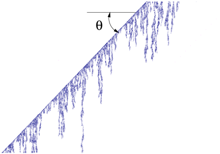
FIG. 1.: The curtain of active sites at the active slanted boundary

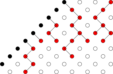
FIG. 2.: Lattice structure near the active boundary

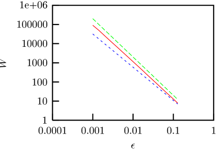
FIG. 3.: Log plot of active width versus $p_{c}-p$ from straight Monte Carlo simulations on unlimited system sizes. The solid line represents the data. The dashed straight lines of slopes $-2$ and $-1.734$ are guides to the eyes.

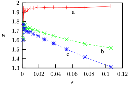
FIG. 4.: Estimates for the active width exponent, $x$. In fit (a), $W$ is assumed to scale as $W\sim\epsilon^{-x}$, in (b), as $W\sim\epsilon^{-x}\ln\epsilon$ and in (c), as $W\sim\epsilon^{-x}(\ln\epsilon+\ln 2)$.

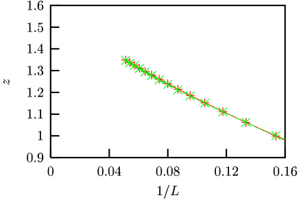
FIG. 5.: Finite size scaling exponent $z$ for ($\times$) the characteristic active width, $W\sim L^{z}$, and for ($+$) the time to reach the stationary state, $t\sim L^{z}$, at the percolation threshold in the transfer matrix set-up. The data virtually coincide

REFERENCES

- [1] W. Kinzel 1983 Percolation Structures and Processes (Ann. Isr. Phys. Soc. 5) ed G. Deutscher, R. Zallen & J. Adler (Bristol:Hilger)
- [2] F. Schlogl, Z. Phys. 253 (1972) 147
- [3] P. Grassberger & A. de la Torre, Ann. Phys. NY 122 (1979) 373
- [4] P. Grassberger & K. Sundermeyer, Phys. Lett. 77B (1978) 220
- [5] R. M. Ziff, E. Gulari & Y. Barshad, Phys. Rev. Lett. 56 (1986) 2553
- [6] I. Jensen, J. Phys. A29 (1996) 7013
- [7] J. W. Essam, A. J. Guttmann, I. Jensen & D. TanlaKishani, J. Phys. A29 (1996) 1619
- [8] P. Frojdh, M. Howard & K. B. Lauritsen, J. Phys. A31 (1998) 2311
- [9] K. B. Lauritsen, P. Frojdh & M. Howard, Phys. Rev. Lett. 81 (1998) 2104
- [10] K. B. Lauritsen, K. Sneppen, M. Markosova & M. H. Jensen, Physica A247 (1997) 1
- [11] S. Kwon, W. Hwang & H. Park, Phys. Rev. E 59 (1999) xxxx.
- [12] W. Klein & W. Kinzel, J. Phys. A14 (1981) L163
- [13] E. Domany & W. Kinzel, Phys. Rev. Lett. 53 (1984) 311
- [14] Chun-Chung Chen, unpublished, based on: J. L. Cardy & R. L. Sugar, J. Phys. A13 (1980) L423, and H. Hinrichsen & H. M. Koduvely, Eur. Phys. J. B5 (1998) 257.