[

Sliding Phases in XY-Models, Crystals, and Cationic Lipid-DNA Complexes

Abstract

We predict the existence of a totally new class of phases in weakly-coupled, three-dimensional stacks of two-dimensional ($2$D) $XY$-models. These “sliding phases” behave essentially like decoupled, independent $2$D $XY$-models with precisely zero free energy cost associated with rotating spins in one layer relative to those in neighboring layers. As a result, the two-point spin correlation function decays algebraically with in-plane separation. Our results, which contradict past studies because we include higher-gradient couplings between layers, also apply to crystals and may explain recently observed behavior in cationic lipid-DNA complexes.
Pacs: 61.30.Cz,61.30.Jf,64.70.Md

]

Spatial dimensionality greatly affects the nature of order in condensed matter systems. Three-dimensional ($3$D) $XY$-systems such as superfluids and ferromagnets have true long-range order with divergent correlation lengths at a second-order transition separating the high-temperature disordered phase from the low-temperature ordered phase. Two-dimensional ($2$D) $XY$-systems, in contrast, exhibit power-law decay of correlations in the low-temperature phase. At high temperatures beyond the Kosterlitz-Thouless (KT) transition temperature, thermally excited vortices destroy the quasi-long-range order and cause correlations to decay exponentially[1, 2].

Many experimentally realizable systems such as layered superconductors[3], free-standing liquid-crystal films[4], and lyotropic smectics with internal membrane order can be viewed as stacks of two-dimensional layers with interlayer couplings [5] that can be varied substantially, for example by changing the layer spacing. What is the phase behavior of such a system? If there is no coupling between layers, each will exhibit $2$D behavior; if the coupling is strong, the system will exhibit $3$D behavior. Shortly after the discovery of the KT transition, it was suggested that a weakly-coupled stack of $XY$-models might behave over some temperature range as a stack of decoupled layers, i.e., that such a system could proceed from three-dimensional behavior at low temperatures to a $2$D power-law phase at intermediate temperatures to a disordered phase at high temperatures[3, 6].

Subsequent studies, however, demonstrated that if the only interlayer couplings are Josephson (i.e., proportional to $\cos(\theta_{n}-\theta_{n+1})$, where $\theta_{n}$ is the $XY$-angle variable in layer $n$), the intermediate $2$D power-law phase is squeezed out, and the system goes directly from the $3$D long-range ordered phase to the disordered one with increasing temperature. This happens because the “decoupling temperature” $T_{d}$ above which the Josephson coupling becomes irrelevant is greater than the Kosterlitz-Thouless temperature $T_{KT}$ below which the $2$D ordered phase is stable against vortex unbinding. Thus, the temperature window $T_{d}<T<T_{KT}$ over which the $2$D sliding phase can exist disappears.

In this paper, we revisit this old and seemingly dead issue and show that a thermodynamically stable phase exhibiting $2$D power-law correlations is in fact possible. The new ingredient in our analysis, which was not present in previous treatments, is competing higher-order gradient couplings between layers[7]. These gradient couplings, in the absence of Josephson couplings between layers, produce two-point correlation functions that are identical in form to those of a stack of decoupled $2$D layers. We will refer to this phase as a sliding and not a decoupled phase because the $XY$-angle variables in different layers can slide relative to each other without changing the energy of the system and because nonzero couplings between layers (though not of the Josephson type) are, in fact, present in our model, and furthermore, necessary for the existence of this phase. Remarkably, it is possible through judicious tuning of interlayer gradient couplings to satisfy $T_{d}<T_{KT}$ and produce a stable sliding phase for $T_{d}<T<T_{KT}$.

This investigation into whether or not a sliding phase of $XY$-models exists was inspired by recent work on the possible sliding columnar phase in cationic lipid-DNA complexes[8]. In these complexes, DNA molecules are intercalated between lipid bilayers and, within each layer, the molecules are situated on a one-dimensional lattice. Experiments may be consistent with the existence of a sliding columnar phase in which lattices in neighboring layers are able to slide over each other without energy cost[9] in complete analogy to the sliding phase just described for $XY$-models. Indeed, we have shown theoretically, by methods analogous to those presented here, that it is possible to have a sliding columnar phase in these complexes and, in addition, possible to have a sliding phase in a layered crystal. Details on these two systems will be presented in a future publication[10]; for the remainder of this paper, we will focus on $XY$-models.

The traditional theory for a stack of $XY$-models begins with sum of independent $XY$-Hamiltonians

$${\cal H}_{0}={K\over 2}\sum_{n}\int d^{2}r\left[{\mbox{\boldmath{$\nabla$}}}_{\perp}\theta_{n}({\bf r})\right]^{2},$$ (1)

where ${\bf r}=(x,y,0)$ is a point in the $x$-$y$ plane and ${\mbox{\boldmath{$\nabla$}}}_{\perp}$ is the gradient operator acting on these two coordinates. Josephson-like couplings between layers are then added; these are given by

$${\cal H}_{J}[s_{n}]=-V_{J}[s_{n}]\int d^{2}r\cos\left[\sum_{p}s_{p}\theta_{n+p}({\bf r})\right],$$ (2)

where $s_{n}$ is an integer-valued function of layer number $n$ satisfying $\sum_{n}s_{n}=0$ if there are no external fields inducing long-range order. If all $V_{J}[s_{n}]$ are zero, then in the low-temperature phase $\langle\theta_{n}^{2}({\bf r})\rangle_{0}=\eta\log(L/b)$ and $\cos[\theta_{n}({\bf r})-\theta_{n}(0)]\sim r^{-\eta}$, where

$$\eta={T\over 2\pi K},$$ (3)

$L$ is the sample width, $b$ is a short-distance cutoff in the $x$-$y$ plane, and $\langle.\rangle_{0}$ refers to an average with respect to ${\cal H}_{0}$. The averages of the Josephson Hamiltonians with respect to ${\cal H}_{0}$ scale as $\langle{\cal H}_{J}[s_{n}]\rangle\sim L^{2-\eta[s_{n}]}$ where $\eta[s_{n}]={\eta\over 2}\sum_{p}s_{p}^{2}$. Clearly, the most relevant Josephson coupling is the one with the smallest value of $\eta[s_{n}]$, which results when $s_{n}$ is non-zero on the smallest number of planes. Since $\sum_{n}s_{n}=0$, the smallest value of $\eta[s_{n}]$ is obtained for couplings between two layers separated by $p$ layers with $s_{n}=s_{n}^{p}=\delta_{n,0}-\delta_{n,p}$. For these two-layer couplings, $\eta^{p}=\eta[s_{n}^{p}]=\eta$ for all values of $p$. Thus, the decoupling temperature above which all Josephson couplings are irrelevant is $T_{d}=4\pi K$. The $2D$ KT transition for decoupled layers is $T_{KT}=\pi K/2$; this implies $T_{KT}/T_{d}=1/8<1$, and there is no decoupled phase with power-law correlations.

Josephson couplings are not, however, the only ones permitted by symmetry. Gradients of $\theta_{n}$ in different layers may also be coupled. The Hamiltonian for the ideal sliding phase is ${\cal H}_{S}={\cal H}_{0}+{\cal H}_{g}$, where

$${\cal H}_{g}={1\over 2}\sum_{n,m}\int d^{2}r~{}{U_{m}\over 2}\left[{\mbox{\boldmath{$\nabla$}}}_{\perp}\left(\theta_{n+m}({\bf r})-\theta_{n}({\bf r})\right)\right]^{2}.$$ (4)

This Hamiltonian is invariant with respect to $\theta_{n}({\bf r})\rightarrow\theta_{n}({\bf r})+\psi_{n}$ for any constant $\psi_{n}$, i.e., the energy is unchanged when angles in different layers slide relative to one another by arbitrary amounts. The sliding Hamiltonian can be written as

$${\cal H}_{S}={1\over 2}\sum_{nn^{\prime}}\int d^{2}r~{}K_{nn^{\prime}}{\mbox{\boldmath{$\nabla$}}}_{\perp}\theta_{n}({\bf r})\cdot{\mbox{\boldmath{$\nabla$}}}_{\perp}\theta_{n^{\prime}}({\bf r}),\\$$ (5)

where $K_{nn^{\prime}}=Kf_{n-n^{\prime}}$ with $f_{n}=(1+\sum_{m}\gamma_{m})\delta_{n,0}-\frac{1}{2}\sum_{m}\gamma_{m}(\delta_{n,m}+\delta_{n,-m})$ and $\gamma_{m}=U_{m}/K$. Also, the Fourier transform

$$f(k)=1+\sum_{m}\gamma_{m}(1-\cos km)$$ (6)

of the reduced coupling $f_{n}$ will be used extensively below.

Correlations in the sliding phase can easily be calculated from Eq. (5). We find

$$\langle\theta_{n}({\bf r})\theta_{n^{\prime}}({\bf r}^{\prime})\rangle_{S}=\eta f^{-1}_{n-n^{\prime}}[\ln(L/b)-E(|{\bf r}-{\bf r}^{\prime}|)],$$ (7)

where $\langle\cdot\rangle_{S}$ is an average with respect to ${\cal H}_{S}$ and $E(r)=\int dq[1-J_{0}(qr)]/q$ tends to zero as $r\rightarrow 0$ and to $\ln(r/b^{\prime})$ with $b^{\prime}/b\approx 0.2$ as $r\rightarrow\infty$. The inverse coupling $f_{p}^{-1}$ is defined by

$$f_{p}^{-1}={1\over\pi}\int_{0}^{\pi}dk{\cos kp\over f(k)}.$$ (8)

Thus we find $\langle\theta_{n}^{2}({\bf r})\rangle_{S}=\eta_{S}(0)\ln(L/b)$ and

$$g_{S}({\bf r},p) \equiv \langle[\theta_{n+p}({\bf r})-\theta_{n}(0)]^{2}\rangle_{S}$$ (9)

$$= 2[\widetilde{\eta}_{S}(p)\ln(L/b)+\eta_{S}(p)\ln(r/b^{\prime})]$$ (10)

for large $r$. The coefficients of the logarithms are

$$\widetilde{\eta}_{S}(p)=\eta(f_{0}^{-1}-f_{p}^{-1})~{}~{}{\rm and}~{}~{}\eta_{S}(p)=\eta f_{p}^{-1}.$$ (11)

Note that $\eta_{S}(p)=\eta\delta_{p,0}$ and ${\widetilde{\eta}}_{S}(p)=\eta(1-\delta_{p,0})$ when ${\cal H}_{g}=0$. Using Eq. (9) we find that the correlation function $G_{S}({\bf r},p)\equiv\left\langle\cos[\theta_{n+p}({\bf r})-\theta_{n}(0)]\right\rangle_{S}$ satisfies

$$G_{S}({\bf r},p) \sim \cases{(L/b)^{-{\widetilde{\eta}}(p)}&$p\neq 0$\cr\left(r/b^{\prime}\right)^{-\eta_{S}(0)}&$p=0$.\cr}$$ (12)

Thus, the two-point spin correlation function for spins in different layers vanishes in the $L\rightarrow\infty$ limit, whereas that for spins in the same layer has exactly the same form as it would for a stack of decoupled layers. Now, however, the exponent $\eta_{S}(0)$ depends on the detailed form of the interlayer gradient couplings via $f(k)$. The two-point spin correlation function is zero for spins in different layers; nonetheless, nonvanishing couplings between layers cause other correlation functions that are zero for the totally decoupled layers to become nonzero.

Having established that the sliding phase (if it has not melted) behaves like a stack of decoupled layers, we now ask what happens when the Josephson interlayer couplings of Eq. (2) are turned on. From Eq. (7), we find that $\langle{\cal H}_{J}[s_{n}]\rangle_{S}\sim L^{2-{\tilde{\eta}}_{S}[s_{n}]}$ where ${\widetilde{\eta}}_{S}[s_{n}]=\eta\sum_{n,n^{\prime}}s_{n}s_{n^{\prime}}f^{-1}_{n-n^{\prime}}$. As for the decoupled case, the minimum value of ${\widetilde{\eta}}_{S}[s_{n}]$ is obtained when $s_{n}=s_{n}^{p}$. Thus the decoupling temperature for couplings with $s_{n}=s_{n}^{p}$ is

$$T_{d}(p)={4\pi K\over f_{0}^{-1}-f_{p}^{-1}}$$ (13)

which depends on $p$. The temperature above which all Josephson couplings are irrelevant is $T_{d}=\max_{p}T_{d}(p)$. We will show later that this maximum over all $p$ is finite.

To prove the stability of the sliding phase, we must show that, for some range of the couplings $U_{m}$, the decoupling temperature $T_{d}$ calculated above is less than $T_{KT}$, the temperature at which vortices unbind. To calculate $T_{KT}$, we must calculate the vortex energy. This calculation in our model is similar to that for decoupled layers. Vortex excitations in individual layers remain well defined when the layers are coupled, although, when couplings are sufficiently strong the system becomes truly three dimensional, and vortices should be viewed as segments of closed vortex loops. Defining ${\bf v}_{n}({\bf r})={\mbox{\boldmath{$\nabla$}}}_{\perp}\theta_{n}({\bf r})$, we have

$$\oint_{\Gamma}{\bf v}_{n}\cdot d{\mbox{\boldmath{$\ell$}}}=2\pi\sum_{l}k_{n,l},$$ (14)

where $k_{n,l}$ is the integer strength of the $l$th vortex in the $n$th layer and $\Gamma$ is a contour in layer $n$ enclosing the vortices. Applying Stokes theorem to Eq. (14) then gives

$${\mbox{\boldmath{$\nabla$}}}_{\perp}\times{\bf v}_{n}=m^{z}_{n}({\bf r}){\hat{z}},$$ (15)

where

$$m^{z}_{n}({\bf r})=2\pi\sum_{l}k_{n,l}\delta^{2}({\bf r}-{\bf r}_{n,l})$$ (16)

is the vortex density in layer $n$ and ${\bf r}_{n,l}$ gives the position of each vortex in the $x$-$y$ plane. We then take the $2$D curl of both sides of Eq. (15) and Fourier transform to find

$${\bf v}_{n}({\bf q}_{\perp})={i\epsilon_{ijz}{q_{\perp j}}m^{z}_{n}({\bf q}_{\perp})\over q_{\perp}^{2}}$$ (17)

Using this result in Eq. (5), we obtain the vortex energy

$$E_{V} = {K\over 2}\sum_{n,n^{\prime}}f_{n-n^{\prime}}\int{d^{2}q_{\perp}\over(2\pi)^{2}}{m^{z}_{n}({\bf q}_{\perp})m^{z}_{n^{\prime}}(-{\bf q}_{\perp})\over q_{\perp}^{2}}$$ (18)

$$= \pi K\sum_{n,n^{\prime}}f_{n-n^{\prime}}\left(\sum_{l}k_{n,l}\right)\left(\sum_{l^{\prime}}k_{n^{\prime},l^{\prime}}\right)\ln(L/b)$$ (20)

$$-\pi K\sum_{n,l,n^{\prime},l^{\prime}}f_{n-n^{\prime}}k_{n,l}k_{n^{\prime},l^{\prime}}E(|{\bf r}_{n,l}-{\bf r}_{n^{\prime},l^{\prime}}|).$$

Since $f_{n-n^{\prime}}$ is a positive definite matrix, this equation implies that in the thermodynamic limit, there must be charge neutrality in each layer, i.e., $\sum_{l}k_{n,l}=0$. The interaction between like-sign vortices in different layers $n$ and $n^{\prime}$ is attractive if $f_{n-n^{\prime}}<0$ and repulsive if $f_{n-n^{\prime}}>0$. Since we assume that individual layers are stable in the absence of couplings between layers, $f_{0}>0$ and like-sign vortices within a single layer repel.

The vortex energy $E_{V}$ and Boltzmann statistics imply that the number of times a given configuration of vortices occurs in the system scales with system size as $L^{2-\eta_{KT}[\sigma_{n}]}$, where

$$\eta_{KT}[\sigma_{n}]={\pi K\over T}\sum_{n,n^{\prime}}f_{n-n^{\prime}}\sigma_{n}\sigma_{n^{\prime}},$$ (21)

$\sigma_{n}\equiv\sum_{\ell}k_{n,l}$, and the factor of $L^{2}$ counts the number of places in the $2$D plane the configuration can be placed. Clearly, if $\eta[\sigma_{n}]<2$, the particular vortex configuration $\{\sigma_{n}\}$ will proliferate. The “Kosterlitz-Thouless unbinding” for $\{\sigma_{n}\}$ therefore occurs at a temperature

$$T_{KT}[\sigma_{n}]={\pi K\over 2}\sum_{n,n^{\prime}}f_{n-n^{\prime}}\sigma_{n}\sigma_{n^{\prime}}.$$ (22)

If there is only one vortex in layer $0$, then $\sigma_{n}\equiv\sigma_{n}^{0}=\delta_{n,0}$ and $T_{KT}[\sigma_{n}^{0}]=\pi Kf_{0}/2$. If there is a $+1$ vortex in layer zero and a $\pm 1$ vortex in layer $p$, $\sigma_{n}\equiv\sigma_{n}^{p\pm}=\delta_{n,0}\pm\delta_{n,p}$ and $T_{KT}[\sigma_{n}^{p\pm}]=\pi K(f_{0}\pm f_{p})$. Note that when $f_{p}$ is nonzero $T_{KT}[\sigma_{n}^{p\pm}]$ is not twice $T_{KT}[\sigma_{n}^{0}]$. In fact it is possible for $T_{KT}[\sigma_{n}]$ to be less than $T_{KT}[\sigma_{n}^{0}]$ for one or more configurations $\{\sigma_{n}\}$. The interactions between layers lead to composite multi-layer vortices that cost less energy to create than a single vortex in an individual layer. Unbinding of bound pairs of any set of individual-layer or composite vortices will destroy the rigidity within those layers. Thus, the transition temperature to the disordered state is $T_{KT}=\min_{\{\sigma_{n}\}}T_{KT}[\sigma_{n}]$, and the sliding phase exists provided

$$\beta={T_{KT}\over T_{d}}={\min_{\sigma_{n}}T_{KT}[\sigma_{n}]\over\max_{p}T_{d}(p)}>1.$$ (23)

We will now discuss how the interlayer gradient potentials $U_{m}$ can be chosen so that $\beta>1$. The basic strategy is to choose the $U_{m}$ so that $f(k)$ has a minimum near zero at some value of $k$. We consider a model with both first- and second-neighbor interactions. We ensure that there is a minimum in $f(k)$ at $k_{0}$ by requiring

$$f(k_{0})=1+\gamma_{1}\left(1-\cos k_{0}\right)+\gamma_{2}\left(1-\cos 2k_{0}\right)=\Delta$$ (24)

and $f^{\prime}(k_{0})=0$. These two conditions determine $\gamma_{1}$ and $\gamma_{2}$ in terms of $k_{0}$ and $\Delta$. In the range of $k_{0}$ and $\Delta$ we consider, $\gamma_{1}>0>\gamma_{2}$ and $\gamma_{1}>|\gamma_{2}|$. The minimum can be tuned to zero by taking $\Delta$ to zero, in which case $f(k_{0})=0$ but $f(k)>0$ for all $k\neq k_{0}$. For small $\Delta$, $f_{0}^{-1}-f_{p}^{-1}$ is dominated by values of $k$ near $k_{0}$, and we have

$$f^{-1}_{0}-f^{-1}_{p} \approx {1-\cos(pk_{0})e^{-p\sqrt{\Delta/C}}\over\sqrt{C\Delta}}$$ (25)

$$\approx {p\over C}+{(pk_{0}-2\pi l)^{2}\over 2\sqrt{\Delta C}},$$ (26)

where the final form is valid for $pk_{0}\sim 2\pi l$, $l$ is an integer, and $C=f^{\prime\prime}(k_{0})/2$. From Eq. (25), we see that there exists a curve $T_{d}(p,k_{0})\sim[p/C+(pk_{0}-2\pi l)^{2}/2\sqrt{\Delta C}]^{-1}$ for each value of $p$ that specifies the decoupling temperature as a function of $k_{0}$. For fixed $k_{0}$, $\max_{p}T_{d}(p,k_{0})$ occurs at $p=[2\pi l/k_{0}]$ if $0\leq\{2\pi l/k_{0}\}\leq 1/2$ and at $p=[2\pi l/k_{0}]+1$ if $1/2<\{2\pi l/k_{0}\}<1$, where $[x]$ is the greatest integer less than or equal to $x$ and $\{x\}=x-[x]$ is the fractional part of $x$. As a function of $k_{0}$ near $2\pi l/p$, $T_{d}(p,k_{0})$ reaches a maximum at $k_{0}=2\pi l/p$ and decreases sharply away from this point. Also, in the range of $k_{0}$ and $\Delta$ we have considered, we can prove that composite like-sign vortices in nearest-neighbor planes $p$ and $p+1$ with $\sigma_{n}=\delta_{n,p}+\delta_{n,p+1}$ are the first to unbind and thus $T_{KT}=\pi K(f_{0}+f_{1})=\pi K(1+\gamma_{1}/2+\gamma_{2})$. Since $T_{KT}$ is a smooth function of $k_{0}$, we find that $\beta=T_{KT}/T_{d}$ has sharply-peaked minima at $k_{0}=2\pi l/p$. Direct evaluation of $\beta$ for $\Delta=10^{-5}$ yields $\beta>1$ in the range $0.24<k_{0}/\pi<0.40$ as shown in Fig. 1.

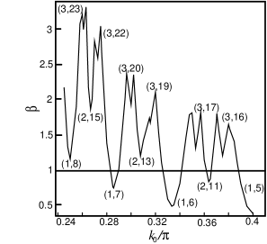
FIG. 1.: $\beta=T_{KT}/T_{d}$ is plotted versus $k_{0}/\pi$. Local minima near $k_{0}/\pi=2l/p$ are labeled by $(l,p)$. Other possible integer pairs either do not fall in the range $0.24<k_{0}/\pi<0.40$ or yield larger values of $\beta$ than those shown above.

Transitions out of the sliding phase are of the Kosterlitz-Thouless or roughening type. The transition to the high-temperature disordered phase at $T_{KT}$ is controlled by $K$ and the fugacity $y_{++}$ for composite like-sign vortices in neighboring layers. The transition to the low-temperature $3D$ ordered phase is controlled by the first $V_{p}\equiv V_{J}[s_{n}^{p}]$ to become relevant and by $U_{p}$.

As we have seen, the Josephson couplings $V_{p}$ are irrelevant with respect to the sliding phase for $T_{d}<T<T_{KT}$. If all $V_{p}$ are set to zero, the two-point correlation function $G_{S}({\bf r},p)$ vanishes for $p\neq 0$. Even though the $V_{p}$ are irrelevant, they are not zero. They give rise to nonzero perturbative contributions to $G_{S}({\bf r},p)$ even when $p$ is nonzero. Consider for simplicity the nearest-neighbor Josephson model ($V_{p}=V\delta_{p,1}$). Then

$$G_{S}({\bf r},p)=\left(V\over 2T\right)^{p}\int d^{2}r_{1}\ldots d^{2}r_{p}e^{-\Phi({\bf r}_{1},\ldots,{\bf r}_{p},{\bf r})/2},$$ (27)

where $\Phi({\bf r}_{1},\ldots,{\bf r}_{p},{\bf r})=\langle[\Delta\theta_{0}(0,{\bf r}_{1})+\Delta\theta_{1}({\bf r}_{1},{\bf r}_{2})+\ldots+\Delta\theta_{p}({\bf r}_{p},{\bf r})]^{2}\rangle_{S}$ and $\Delta\theta_{n}({\bf r}_{1},{\bf r}_{2})=\theta_{n}({\bf r}_{1})-\theta_{n}({\bf r}_{2})$. Using the fact that the transition at $T_{d}^{+}$ is a KT transition, it can be shown that Eq. (27) yields an exponential decay of correlations with $G_{S}(0,p)\sim e^{-p/\xi_{z}}$. The interlayer correlation length $\xi_{z}$ diverges as $T\rightarrow T_{d}^{+}$ according to $\xi_{z}\propto 1/(T-T_{d})$, i.e. the interlayer correlation length exponent is $\nu_{z}=1$. This divergence signals the development of true long-range orientational order in the $3$D ordered phase below $T_{d}$. The derivation of this result will be presented in a forthcoming publication [10].

The ideas presented here can also be applied to a three-dimensional stack of two-dimensional crystals[10]. An interaction Hamiltonian analogous to ${\cal H}_{g}$ in Eq. (4) that couples gradients of displacements in different layers can be introduced. Power-law exponents and dislocation energies again depend on these couplings, and a sliding crystal phase between a low-temperature crystalline and a higher-temperature hexatic phase[11] is possible. The sliding crystal phase is similar to a model once proposed for the smectic B phase in liquid crystals[12]. Also, interlayer gradient couplings for the hexatic angle can be introduced to produce a sliding hexatic phase. Thus the phase sequence $3$D crystal $\rightarrow$ sliding crystal $\rightarrow$ $3$D hexatic $\rightarrow$ sliding hexatic $\rightarrow$ disordered layers is in principle possible in lamellar systems.

This work was supported in part by the National Science Foundation under grants DMR97–30405 and DMR–9634596. J. T. and T. C. L. thank the Aspen Center for Physics for their Winter Meeting, at which this work was initiated. We are also grateful to C. Kane for emphasizing the possibility of melting via composite vortices.

REFERENCES

[1]
J. M. Kosterlitz and D. J. Thouless, J. Phys. C 6, 1181 (1973).
[2]
D. R. Nelson and B. I. Halperin, Phys. Rev. B 19, 2457 (1979);
A. P. Young, Phys. Rev. A 19, 1855 (1979).
[3]
B. Horovitz, Phys. Rev. B 45, 12632 (1992).
[4]
P. S. Pershan, Structure of Liquid Crystal Phases (World Scientific,
Singapore, 1988).
[5]
I. Koltover, J. O. Rädler, T. Salditt, K. J. Rothschild, and
C. R. Safinya, Phys. Rev. Lett. 82, 3184 (1999).
[6]
S. Hikami and T. Tsuneto, Prog. of Theoretical Phys. 63, 387 (1980).
[7]
E. Granato and J. M. Kosterlitz, Phys. Rev. B 33, 4767 (1986)
introduce such couplings between two coupled -models.
[8]
C.S. O’Hern and T.C. Lubensky, Phys. Rev. Lett. 80, 4345 (1998);
L. Golubović and M. Golubović, Phys. Rev. Lett. 80, 4341 (1998).
[9]
T. Salditt, I. Koltover, J.O. Rädler, and C.R. Safinya,
Phys. Rev. Lett. 79, 2582 (1997); F. Artzner, R. Zantl, G. Rapp,
and J.O. Rädler, Phys. Rev. Lett. 81, 5015 (1998).
[10]
C. S. O’Hern, T.C. Lubensky, and J. Toner (unpublished).
[11]
R. J. Birgeneau and J. D. Litster, J. Phys. Lett. (Paris) 39,
399 (1978).
[12]
P. G. De Gennes and G. Sarma, Phys. Lett. 38A, 219 (1972).