Exact Finite Size Study of the
2dOCP at $\Gamma=4$ and $\Gamma=6$

G. Téllez
Ecole Normale Supérieure de Lyon, Laboratoire de Physique,
Unité Mixte de Recherche 5672 du Centre National de la Recherche Scientifique,
46, allée d’Italie, 69364 Lyon Cedex 07, France

P.J.Forrester
Department of Mathematics and Statistics, University of Melbourne,
Parkville, Victoria 3052, Australia

An exact numerical study is undertaken into the finite $N$ calculation of the free energy and distribution functions for the two-dimensional one-component plasma. Both disk and sphere geometries are considered, with the coupling $\Gamma$ set equal to 4 and 6. Extrapolation of our data for the free energy is consistent with the existence of a universal term ${\chi\over 12}\log N$, where $\chi$ denotes the Euler characteristic of the surface, as predicted theoretically. The exact finite $N$ density profile is shown to give poor agreement with the contact theorem relating the density at contact and potential drop to the pressure in the thermodynamic limit. This is understood theoretically via a known finite $N$ version of the contact theorem. Furthermore, the ideas behind the derivation of the latter result are extended to give a sum rule for the second moment of the pair correlation in the finite disk, which in the thermodynamic limit converges to the Stillinger-Lovett result.

1 Introduction

The two-dimensional one-component plasma (2dOCP) is a model in classical statistical mechanics which consists of $N$ mobile point particles of charge $q$ interacting on a surface with uniform neutralizing background charge density. The pair potential $\Phi(\vec{r},\vec{r}\,^{\prime})$ between particles is the solution of the Poisson equation on the particular surface. In the plane

$$\Phi(\vec{r},\vec{r}\,^{\prime})=-\log\Big{(}|\vec{r}-\vec{r}\,^{\prime}|/l\Big{)},$$ (1.1)

where $l$ is some arbitrary length scale which will henceforth be set to unity. With the potential (1.1) and a uniform background of charge density $-\rho_{b}$ inside a disk of radius $R$ $(\rho_{b}=N/\pi R^{2})$ the corresponding Boltzmann factor, which consists of the particle-particle, particle-background and background-background interaction, is given by

$$e^{-\Gamma N^{2}((1/2)\log R-3/8)}e^{-\pi\Gamma\rho_{b}\sum_{j=1}^{N}|\vec{r}_{j}|^{2}/2}\prod_{1\leq j<k\leq N}|\vec{r}_{k}-\vec{r}_{j}|^{\Gamma},$$ (1.2)

where $\Gamma:=q^{2}/k_{B}T$ is the coupling. We remark that with $\Gamma/2$ an odd integer, (1.2) is proportional to the absolute value squared of the celebrated Laughlin trial wave function for the fractional quantum Hall effect [Lau83].

At the analytic level our knowledge of the properties of the 2dOCP comes from two main sources. First, for the special coupling $\Gamma=2$, the exact free energy and correlation functions can be calculated for a number of different geometries [AJ81, Cho81, Cai81, JT98]. Second, the 2dOCP is an example of a Coulomb system in its conductive phase and as such should obey a number of sum rules (see e.g. [Mar88]) which typically represent universal properties of such a system. We remark also that the exact solutions at $\Gamma=2$ have been an important source of inspiration to identify universal properties.

In this paper we develop exact numerical solutions at the special couplings $\Gamma=4$ and $\Gamma=6$ for values of $N$ up to 11 and 9 respectively. By undertaking this study we are able to test the prediction of Jancovici et al. [JMP94] that the expression for the free energy $F$ as a function of the number of particles $N$ be of the form

$$\beta F=AN+BN^{1/2}+{\chi\over 12}\log N+\cdots,$$ (1.3)

where $\chi$ denotes the Euler characteristic of the surface ($\chi=1$ for a disk, $\chi=2$ for a sphere). Furthermore we are able to investigate the rate of convergence of the one and two point correlation to their thermodynamic values, as well as the accuracy of certain sum rules in the finite system. In fact the latter line of investigation leads us to a new sum rule valid for general $\nu$ dimensional multicomponent Coulomb systems in a spherical domain, which relates to the second moment of the density-charge correlation function in the finite system. We recall (see e.g. [Mar88]) that in the infinite system the second moment of the charge-charge correlation function is of a universal form known as the Stillinger-Lovett condition. Indeed our sum rule (4.24) below gives the finite size correction to this universal form in systems with a background.

As an outline of the paper, we note here that in Section 2 formulas are presented specifying the partition function and one and two point distribution functions for the disk and sphere geometries, with the coupling an even integer, in terms of certain expansion coefficients. These expansion coefficients are in general computationally expensive, but reasonably efficient algorithms exist in the literature applicable to the cases $\Gamma=4$ and 6. Our numerical results our presented in Section 3. The new sum rules are derived and discussed in Section 4, while Section 5 concludes with a summary.

2 Formalism

Our interest is in the exact numerical computation of the partition function and one and two-point correlation functions for the 2dOCP in a disk and on the surface of a sphere. In the former system the Boltzmann factor is given by (1.1). Two versions of this model will be considered: one in which the particles are confined to a disk of radius $R$ (the same disk which contains the smeared out neutralizing background), and the other in which the particles are can move throughout the plane. These will be referred to as the hard disk and soft disk respectively. In the latter system the Boltzmann factor (1.1) is assumed valid also for $|\vec{r}_{i}|\geq R$, even though the one body potential $\pi\rho_{b}|\vec{r}_{i}|^{2}/2$ is not the correct potential for the coupling between a particle and the background in this region (according to Newton’s theorem outside the disk the background creates the same potential as a charge $-N$ at the origin, so the correct Coulomb potential outside the disk is $N\log|\vec{r}_{i}|$).

On the surface of the sphere the Boltzmann factor is given by

$${\left({1\over{2R}}\right)}^{N\Gamma/2}e^{\Gamma N^{2}/4}\prod_{1\leq j<k\leq N}{|u_{k}v_{j}-u_{j}v_{k}|}^{\Gamma},$$ (2.1)

where $u:=\cos(\theta/2)e^{i\phi/2},\ v:=-i\sin(\theta/2)e^{-i\phi/2}$ are the Cayley-Klein parameters and $(\theta,\phi)$ are the usual spherical coordinates. For our purpose it is convenient to consider the stereographic projection of this system from the south pole of the sphere to the plane tangent to the north pole. This is specified by the equation

$$z=2Re^{i\phi}\tan{\theta\over 2},\qquad z=x+iy.$$ (2.2)

We then have

$${\left({1\over{2R}}\right)}^{N\Gamma/2}e^{\Gamma N^{2}/4}\prod_{1\leq j<k\leq N}{|u_{k}v_{j}-u_{j}v_{k}|}^{\Gamma}dS_{1}\cdots dS_{N}={\left({1\over{2R}}\right)}^{N\Gamma/2}$$ (2.3)

$$\times e^{\Gamma N^{2}/4}\prod_{j=1}^{N}{1\over(1+|z_{j}|^{2}/(4R^{2}))^{2+\Gamma(N-1)/2}}\prod_{1\leq j<k\leq N}\left|\frac{z_{j}-z_{k}}{2R}\right|^{\Gamma}d\vec{r}_{1}\cdots d\vec{r}_{N}.$$

2.1 The cases $\Gamma=4p$

For $\Gamma=4p$, integrals over the Boltzmann factors (1.1) and (2.3) can be performed from knowledge of the coefficients in the expansion

$$\prod_{1\leq j<k\leq N}(z_{k}-z_{j})^{2p}=\sum_{\mu}c_{\mu}^{(N)}(2p)m_{\mu}(z_{1},\dots,z_{N})$$ (2.4)

where $\mu=(\mu_{1},\dots,\mu_{N})$ is a partition of $pN(N-1)$ such that

$$2p(N-1)\geq\mu_{1}\geq\cdots\mu_{N}\geq 0$$

and

$$m_{\mu}(z_{1},\dots,z_{N})={1\over\prod_{i}m_{i}!}\sum_{\sigma\in S_{N}}z_{\sigma(1)}^{\mu_{1}}\cdots z_{\sigma(N)}^{\mu_{N}}$$

is the corresponding monomial symmetric function (the $m_{i}$ denote the frequency of the integer $i$ in the partition). The key point for the utility of (2.4) is that with $z_{j}=r_{j}e^{i\theta_{j}}$, the $m_{\mu}$ are orthogonal with respect to angular integrations:

$$\int_{0}^{\infty}dr_{1}\,r_{1}g(r_{1}^{2})\cdots\int_{0}^{\infty}dr_{N}\,r_{N}g(r_{N}^{2})\int_{0}^{2\pi}d\theta_{1}\cdots\int_{0}^{2\pi}d\theta_{N}\,m_{\mu}(z_{1},\dots,z_{N})\overline{m_{\kappa}(z_{1},\dots,z_{N})}$$

$$=\delta_{\mu,\kappa}{N!\over\prod_{i}m_{i}!}\pi^{N}\prod_{l=1}^{N}G_{\mu_{l}}\hskip 56.9055pt$$ (2.5)

where $G_{\mu_{l}}:=2\int_{0}^{\infty}dr\,r^{1+2\mu_{l}}g(r^{2})$ for arbitrary $g(r^{2})$. Thus, after also noting that

$$\prod_{j<k}|z_{k}-z_{j}|^{4p}=\prod_{j<k}(z_{k}-z_{j})^{2p}\prod_{j<k}(\bar{z}_{k}-\bar{z}_{j})^{2p},$$ (2.6)

we see that for $\Gamma=4p$

$$I_{N,\Gamma}[g]:=\int_{{\mathbf{R}}^{2}}d\vec{r}_{1}\,g(r_{1}^{2})\cdots\int_{{\mathbf{R}}^{2}}d\vec{r}_{N}\,g(r_{N}^{2})\,\prod_{j<k}|\vec{r}_{k}-\vec{r}_{j}|^{\Gamma}=N!\pi^{N}\sum_{\mu}{(c_{\mu}^{(N)}(2p))^{2}\over\prod_{i}m_{i}!}\prod_{l=1}^{N}G_{\mu_{l}}.$$ (2.7)

In the case $p=1$ this formalism has been utilized by Samaj et al. [SPK94], who furthermore presented an algorithm for the computation of $\{c_{\mu}\}$ in this case. Let us now consider this latter point.

In general the coefficients $c_{\mu}^{(N)}(2p)$ can be calculated from the formula

$$c_{\mu}^{(N)}(2p)={1\over(2\pi)^{N}}\int_{0}^{2\pi}d\theta_{1}\,e^{-i\mu_{1}\theta_{1}}\cdots\int_{0}^{2\pi}d\theta_{N}e^{-i\mu_{N}\theta_{N}}\prod_{j<k}(e^{i\theta_{k}}-e^{i\theta_{j}})^{2p},$$ (2.8)

which follows from (2.4). Since we require $|\mu|=pN(N-1)$, the integral over $\theta_{N}$ can be performed by changing variables $\theta_{j}\mapsto\theta_{j}+\theta_{N}$ $(j=1,\dots,N-1)$ to give

$$c_{\mu}^{(N)}(2p) = {1\over(2\pi)^{N-1}}\int_{0}^{2\pi}d\theta_{1}\,e^{-i\mu_{1}\theta_{1}}\cdots\int_{0}^{2\pi}d\theta_{N-1}e^{-i\mu_{N-1}\theta_{N-1}}\prod_{j=1}^{N-1}(1-e^{i\theta_{j}})^{2p}$$ (2.9)

$$\times\prod_{1\leq j<k\leq N-1}(e^{i\theta_{k}}-e^{i\theta_{j}})^{2p}.$$

The simplest case is $N=2$, when the sum over pairs in (2.9) is not present. Expanding $(1-e^{i\theta_{1}})^{2p}$ according to the binomial theorem gives

$$c_{\mu}^{(2)}(2p)=(-1)^{\mu_{1}}\left({2p\atop\mu_{1}}\right)$$

where $\mu_{1}=p,p+1,\dots,2p$ (for $\mu_{1}=p$ we have $\mu_{1}=\mu_{2}$ and thus $m_{\mu_{1}}=2$, while in all other cases $\mu_{1}\neq\mu_{2}$ and so $m_{\mu_{1}}=m_{\mu_{2}}=1$). Substituting in (2.7) we see, after some minor manipulation, that

$$\int_{{\mathbf{R}}^{2}}d\vec{r}_{1}\,g(r_{1}^{2})\int_{{\mathbf{R}}^{2}}d\vec{r}_{2}\,g(r_{2}^{2})\,|\vec{r}_{2}-\vec{r}_{1}|^{4p}=\pi^{2}\sum_{\mu=0}^{2p}\left({2p\atop\mu}\right)^{2}\int_{0}^{\infty}dr\,r^{\mu}g(r)\int_{0}^{\infty}dr\,r^{2p-\mu}g(r).$$ (2.10)

To calculate $c_{\mu}^{(N)}(2p)$ via this method for a general value of $N$ would require expanding ${1\over 2}(N-1)N$ products via the binomial theorem, giving a total of $({1\over 2}(N-1)N)^{2p+1}$ terms to determine each value of $c_{\mu}$. Thus for a given value of $N$ the complexity increases exponentially with the coupling $p$. As we want to determine the $c_{\mu}$ for a sequence of values of $N$ as large as possible, we are therefore restricted to the case $p=1$.

In fact the case $p=1$ allows (2.8) to be computed without using the binomial expansion [SPK94]. Instead one uses the Vandermonde formula for the product of differences as a determinant to expand the products in (2.8). This gives

$$c_{\mu}^{(N)}(2)=\sum_{P\in S_{N}}\varepsilon(P)\sum_{Q\in S_{N}}\varepsilon(Q)\prod_{k=1}^{N}\delta_{P(k)+Q(k)-2,\mu_{k}}=\sum_{P\in S_{N}}\varepsilon(P)\sum_{Q\in S_{N}}\prod_{k=1}^{N}\delta_{P(k)+k-2,\mu_{Q(k)}},$$ (2.11)

which is the formula we used to compute our data in the case $p=1$ for $N=3,\dots,10$.

2.2 The cases $\Gamma=4p+2$

With $\Gamma=4p+2$, decomposing the product of differences analogous to (2.6) shows that we must consider the product of differences raised to an odd power. The analogue of (2.4) is then the expansion

$$\prod_{1\leq j<k\leq N}(z_{k}-z_{j})^{2p+1}=\sum_{\mu}c_{\mu}^{(N)}(2p+1){\cal A}(z_{1}^{\mu_{1}+N-1}z_{2}^{\mu_{2}+N-2}\cdots z_{N}^{\mu_{N}})$$ (2.12)

where $2p(N-1)\geq\mu_{1}\geq\mu_{2}\geq\cdots\geq\mu_{N}\geq 0$, $\sum_{j=1}^{N}\mu_{j}=pN(N-1)$ and ${\cal A}$ denotes antisymmetrization. Factoring out the antisymmetric factor $\prod_{j<k}(z_{k}-z_{j})$ from both sides then gives

$$\prod_{1\leq j<k\leq N}(z_{k}-z_{j})^{2p}=\sum_{\mu}c_{\mu}^{(N)}(2p+1)S_{\mu}(z_{1},\dots,z_{N})$$ (2.13)

where $S_{\mu}$ denotes the Schur polynomial indexed by the partition $\mu$. Furthermore, analogous to the orthogonality (2.1) we have

$$\int_{0}^{\infty}\cdots\int_{0}^{\infty}\prod_{l=1}^{N}dr_{l}\,r_{l}g(r_{l}^{2})\int_{0}^{2\pi}d\theta_{1}\cdots\int_{0}^{2\pi}d\theta_{N}\prod_{j<k}\left|z_{j}-z_{k}\right|^{2}S_{\mu}(z_{1},\dots,z_{N})\overline{S_{\kappa}(z_{1},\dots,z_{N})}$$

$$=\delta_{\mu,\kappa}N!\pi^{N}\prod_{l=1}^{N}G_{\mu_{l}+N-l}.\hskip 56.9055pt$$ (2.14)

Thus for $\Gamma=4p+2$, instead of (2.7) we have

$$I_{N,\Gamma}[g]=N!\pi^{N}\sum_{\mu}(c_{\mu}^{(N)}(2p+1))^{2}\prod_{l=1}^{N}G_{\mu_{l}+N-l}.$$ (2.15)

According to (2.12) the coefficients $c_{\mu}^{(N)}(2p+1)$ can be computed from the formula (2.8) with $\mu_{j}\mapsto\mu_{j}+N-j$ and $2p\mapsto 2p+1$, or equivalently (2.9) with the same replacements. In the case $N=2$ this latter formula gives

$$c_{\mu}^{(2)}(2p+1)=(-1)^{\mu_{1}+1}\left({2p+1\atop\mu_{1}+1}\right)$$

with $\mu_{1}=p,\dots,2p$. This in turn implies that the formula (2.10) again holds with $2p\mapsto 2p+1$.

To obtain data for consecutive values of $N$, the computationally simplest case is $p=1$. However algorithms based on (2.8) (with $\mu_{j}\mapsto\mu_{j}+N-j$ and $2p\mapsto 2p+1$) are inferior to methods that determine $c_{\mu}^{(N)}(3)$ from (2.13) [FGIL94, Dun94, STW94]. The most efficient algorithm appears to be the one of Scharf et al. [STW94], where the coefficients $c_{\mu}^{(N)}(3)$ are determined up to $N=9$. Fortunately the authors of [STW94] have kindly supplied us with their data (up to $N=8$), so we do not need to repeat the calculation.

2.3 The sphere

The Boltzmann factor for the sphere, stereographically projected onto the plane, is given by the r.h.s. of (2.3). Thus, with ${\vec{r}\,}_{j}\mapsto 2R{\vec{r}\,}_{j}$ we require

$$g(r^{2})=(1+r^{2})^{-(N-1)\Gamma/2-2}$$ (2.16)

in the integral (2.7). However, computational savings can be obtained by first noting that because the sphere is homogeneous, one particle can be fixed at the north pole, reducing the number of integrals from $N$ to $N-1$ (we must also multiply by $\pi$ – the area of the surface of a sphere of radius $1/2$). Thus we have

$$\int_{({\mathbf{R}}^{2})^{N}}d\vec{r}_{1}\cdots d\vec{r}_{N}\,\prod_{i=1}^{N}{1\over(1+|z_{i}|^{2})^{(N-1)\Gamma/2+2}}\prod_{1\leq j<k\leq N}|z_{k}-z_{j}|^{\Gamma}\qquad$$

$$=\pi\int_{({\mathbf{R}}^{2})^{N-1}}d\vec{r}_{1}\cdots d\vec{r}_{N-1}\,\prod_{i=1}^{N-1}{|z_{i}|^{\Gamma}\over(1+|z_{i}|^{2})^{(N-1)\Gamma/2+2}}\prod_{1\leq j<k\leq N-1}|z_{k}-z_{j}|^{\Gamma},$$ (2.17)

and so should choose

$$g(r^{2})={r^{\Gamma}\over(1+r^{2})^{(N-1)\Gamma/2+2}}$$ (2.18)

in (2.7).

With $g(r^{2})$ given by (2.18), the formulas (2.7) and (2.15) show that at $\Gamma=4$ and $\Gamma=6$ the canonical partition function

$$Z_{N,\Gamma}:={1\over N!}\int_{({\mathbf{R}}^{2})^{N}}d\vec{r}_{1}\cdots d\vec{r}_{N}\,e^{-\beta U}$$

can be represented by the series

$$Z_{N+1,4}^{\mathrm{sphere}} = {e^{(N+1)^{2}}\pi^{N+1}\over N+1}\sum_{\nu}\left(c_{\nu}^{(N)}(2)\right)^{2}{1\over\prod_{i}m_{i}!}\prod_{i=1}^{N}{(\mu_{i}+2)!(2N-\mu_{i}-2)!\over(2N+1)!}$$ (2.19)

$$Z_{N+1,6}^{\mathrm{sphere}} = \rho_{b}^{(N+1)/2}(N+1)^{(N+3)/2}e^{3(N+1)^{2}/2}\pi^{3(N+1)/2}\sum_{\nu}(c_{\nu}^{(N)}(3))^{2}$$ (2.20)

$$\times\prod_{k=1}^{N}{(3+N+\mu_{k}-k)!(2N-3-\mu_{k}+k)!\over(3N+1)!}.$$

To obtain these formulas use has been made of the definite integral

$$\int_{0}^{\infty}{r^{p}\over(1+r)^{q}}\,dr={\Gamma(p+1)\Gamma(q-p-1)\over\Gamma(q)}.$$ (2.21)

Because the sphere is homogeneous, the two-point distribution $\rho_{(2)}((\theta,\phi),(\theta^{\prime},\phi^{\prime}))$ can be computed with one particle at the north pole ($\theta^{\prime}=0$ say). We then have

$$\rho_{(2)}((\theta,\phi),\,(\theta^{\prime},\phi^{\prime}))=\rho_{(2)}(\theta)$$

so the two-point function can be computed from an integral of the form (2.7). In fact with $g(r^{2})$ given by (2.16) we have

$$\rho_{(2)}(\theta)=\frac{1}{4R^{2}}\frac{1}{I_{N,\Gamma}[g]}\lim_{x^{\prime}\to 0}\frac{g(x^{2})g({x^{\prime}}^{2})}{4\pi^{2}xx^{\prime}}(1+x^{2})^{2}(1+x^{\prime 2})^{2}\frac{\delta^{2}I_{N,\Gamma}[g]}{\delta g(x^{2})\delta g(x^{\prime 2})}$$ (2.22)

where $x=\tan(\theta/2)$. For $\Gamma=4$ this gives

$$\rho_{(2)}(\theta)=\rho_{b}^{2}\frac{(2N-1)!}{N^{2}(1+x^{2})^{2N-2}}$$ (2.23)

$$\times \frac{\displaystyle\sum_{\mu,\mu_{N}=0}(c_{\mu}^{(N)}(2))^{2}{1\over\prod_{i}m_{i}!}\prod_{i=1}^{N}\mu_{i}!(2N-2-\mu_{i})!\sum_{k=1}^{N-1}\frac{x^{2\mu_{k}}}{\mu_{k}!(2N-2-\mu_{k})!}}{\sum_{\mu}(c_{\mu}^{(N)}(2))^{2}{1\over\prod_{i}m_{i}!}\prod_{i=1}^{N}\mu_{i}!(2N-2-\mu_{i})!}$$

while for $\Gamma=6$ we deduce that

$$\rho_{(2)}(\theta)=\rho_{b}^{2}\frac{(3N-2)!}{N^{2}(1+x^{2})^{3N-3}}\,(3N-2)$$ (2.24)

$$\times \frac{\displaystyle\sum_{\mu,\mu_{N}=0}\!\!(c_{\mu}^{(N)}(3))^{2}\!\prod_{i=1}^{N}\!(\mu_{i}\!\!+\!\!N\!\!-\!\!i)!(2N\!\!-\!\!3\!\!-\!\!\mu_{i}\!\!+\!\!i)!\!\sum_{k=1}^{N-1}\frac{x^{2(\mu_{k}+N-k)}}{(\mu_{k}\!\!+\!\!N\!\!-\!\!k)!(2N\!\!-\!\!3\!\!-\!\!\mu_{k}\!\!+\!\!k)!}}{\sum_{\mu}(c_{\mu}^{(N)}(3))^{2}\prod_{i=1}^{N}(\mu_{i}+N-i)!(2N-3-\mu_{i}+i)!}$$

2.4 The disk

In the case of the disk, (1.2) with $\vec{r}_{j}\mapsto R\vec{r}_{j}$ shows we require

$$g(r^{2})=\chi(r)e^{-\Gamma N|\vec{r}_{j}|^{2}/2}$$ (2.25)

where $\chi=1$ for $r^{2}<1$ and zero otherwise in the case of the hard disk, while $\chi=1$ for all $r$ in the case of the soft disk. Thus from (2.7) we have at $\Gamma=4$

$$Z_{N,4}^{\mathrm{soft\ disk}} = e^{3N^{2}/2}\left(\frac{1}{2N}\right)^{N^{2}}\pi^{N}\sum_{\mu}(c_{\mu}^{(N)}(2))^{2}\left(\prod_{i}m_{i}!\right)^{-1}\prod_{i=1}^{N}\mu_{i}!$$ (2.26)

$$Z_{N,4}^{\mathrm{hard\ disk}} = e^{3N^{2}/2}\left(\frac{1}{2N}\right)^{N^{2}}\pi^{N}\sum_{\mu}(c_{\mu}^{(N)}(2))^{2}{1\over\prod_{i}m_{i}!}\prod_{i=1}^{N}\gamma(\mu_{i}+1,2N)$$ (2.27)

while at $\Gamma=6$ use of (2.15) gives

$$Z_{N,6}^{\mathrm{hard}}=\rho_{b}^{N/2}N^{-3N^{2}/2}3^{-N(3N-1)/2}\pi^{3N/2}e^{9N^{2}/4}\sum_{\mu}(c_{\mu}^{(N)}(3))^{2}\prod_{k=1}^{N}\gamma(\mu_{k}+N-k+1,3N)$$ (2.28)

with the soft disk case obtained by replacing the incomplete gamma functions by complete gamma functions.

Unlike the situation with the sphere, the density is a non-constant function in the disk geometry. Now, with $g(r^{2})$ given by (2.18) we have

$$\rho_{(1)}(r)={g(r^{2})\over 2\pi r}{\delta\log Z_{N,4}^{\mathrm{disk}}\over\delta g(r^{2})}.$$

At $\Gamma=4$ this gives

$$\rho_{(1)}(r)=2\rho_{b}e^{-2\pi\rho_{b}r^{2}}$$ (2.29)

$$\times\frac{\displaystyle\sum_{\mu}(c_{\mu}^{(N)}(2))^{2}{1\over\prod_{i}m_{i}!}\prod_{j=1}^{N}\gamma(\mu_{j}+1,2N)\sum_{k=1}^{N}\frac{(2\pi\rho_{b}r^{2})^{\mu_{k}}}{\gamma(\mu_{k}+1,2N)}}{\sum_{\mu}(c_{\mu}^{(N)}(2))^{2}{1\over\prod_{i}m_{i}!}\prod_{j=1}^{N}\gamma(\mu_{j}+1,2N)}$$

while at $\Gamma=6$ one obtains

$$\rho_{(1)}(r)=3\rho_{b}e^{-3\pi\rho_{b}r^{2}}$$ (2.30)

$$\times\frac{\displaystyle\sum_{\mu}(c_{\mu}^{(N)}(3))^{2}\prod_{j=1}^{N}\gamma(\mu_{j}+N-j+1,3N)\sum_{k=1}^{N}\frac{(3\pi\rho_{b}r^{2})^{\mu_{k}+N-k}}{\gamma(\mu_{k}+N-k+1,3N)}}{\sum_{\mu}(c_{\mu}^{(N)}(3))^{2}\prod_{j=1}^{N}\gamma(\mu_{j}+N-j+1,3N)}$$

The corresponding formulas for the soft disk are obtained by replacing the incomplete gamma functions by complete gamma functions.

Finally, we consider the two-point function in the disk geometry. In general this quantity is not just a function of the distance between particles, and so we cannot use the formalism based on the orthogonalities (2.1) and (2.2). However, with one of the particles fixed at the origin ($\vec{r}\,^{\prime}=\vec{0}$ say) we have $\rho_{(2)}(\vec{r},\vec{r}\,^{\prime})=\rho_{(2)}(r)$, so in this case the formalism used to compute the densities can again be used. Thus using the general formula

$$\rho_{(2)}(r)={1\over Z_{N,\Gamma}}\lim_{r^{\prime}\to 0}{g(r^{2})g({r^{\prime}}^{2})\over 4\pi rr^{\prime}}{\delta^{2}Z_{N,\Gamma}\over\delta g(r^{2})\delta g({r^{\prime}}^{2})},$$

we find for the hard disk case

$$\rho_{(2)}(r)=4\rho_{b}^{2}e^{-2\pi\rho_{b}r^{2}}$$ (2.31)

$$\times\frac{\sum_{\mu,\mu_{N}=0}(c_{\mu}^{(N)}(2))^{2}{1\over\prod_{i}m_{i}!}\prod_{j=1}^{N-1}\gamma(\mu_{j}+1,2N)\sum_{k=1}^{N-1}\frac{(2\pi\rho_{b}r^{2})^{\mu_{k}}}{\gamma(\mu_{k}+1,2N)}}{\sum_{\mu}(c_{\mu}^{(N)}(2))^{2}{1\over\prod_{i}m_{i}!}\prod_{j=1}^{N}\gamma(\mu_{j}+1,2N)}$$

$$\rho_{(2)}(r)=9\rho_{b}^{2}e^{-3\pi\rho_{b}r^{2}}$$ (2.32)

$$\times\frac{\displaystyle\sum_{\mu,\mu_{N}=0}(c_{\mu}^{(N)}(3))^{2}\prod_{j=1}^{N-1}\gamma(\mu_{j}+N-j+1,3N)\sum_{k=1}^{N-1}\frac{(3\pi\rho_{b}r^{2})^{\mu_{k}+N-k}}{\gamma(\mu_{k}+N-k+1,3N)}}{\sum_{\mu}(c_{\mu}^{(N)}(3))^{2}\prod_{j=1}^{N}\gamma(\mu_{j}+N-j+1,3N)}$$

for $\Gamma=4$ and $\Gamma=6$ respectively. Again the corresponding results for the soft disk are obtained by replacing the incomplete gamma functions by complete gamma functions.

3 Numerical results

3.1 Free energy – sphere geometry

In the Introduction it was commented that the free energy is expected to have a large $N$ expansion of the form (1.3) with $\chi=2$ in sphere geometry. In fact the constant $B$ in (1.3), which is a surface free energy, should be identically zero in sphere geometry, so we expect a large $N$ expansion of the form

$$\beta F=AN+{1\over 6}\log N+C+\cdots.$$ (3.1)

As noted by Jancovici et al. [JMP94], the validity of (3.1) can be explicitly demonstrated at $\beta=2$ because of an exact solution due to Caillol [Cai81]. The mechanism for the exact solution can be seen within the present formalism. Thus, at $\Gamma=2$ we require the coefficients $c_{\mu}^{(N)}(1)$ in (2.12). But this follows from the Vandermonde expansion (recall (2.11)), which gives $c_{\mu}^{(N)}(1)=1$ for $\mu=0^{N}$ and $c_{\mu}^{(N)}(1)=0$ otherwise. Substituting in (2.15) with $g(r^{2})$ given by (2.18), and making use of (2.21) we thus obtain [Cai81]

$$Z_{N,2}^{\mathrm{sphere}}=\pi^{-N/2}N^{N/2}\rho_{b}^{-N/2}e^{N^{2}/2}\prod_{k=1}^{N}{(N-k)!(k-1)!\over N!}.$$ (3.2)

This substituted into the general formula

$$\beta F_{N,\Gamma}=-\log Z_{N,\Gamma}$$ (3.3)

leads to the expansion [JMP94]

$$\beta F=Nf+{1\over 6}\log N+{1\over 12}-2\zeta^{\prime}(-1)+{\mathrm{o}}(1)$$ (3.4)

where $f={1\over 2}\log(\rho_{b}/2\pi^{2})$. We remark that by introducing the Barnes $G$ function according to

$$G(z+1)=\Gamma(z)G(z),\quad G(1)=1$$

we can write

$$\prod_{k=1}^{N}(k-1)!=G(N+1).$$

The large $N$ expansion of the Barnes $G$ function is known to be [Bar00]

$$G(N+1)\sim{N^{2}\over 2}\log N-{3\over 4}N^{2}+{N\over 2}\log 2\pi-{1\over 12}\log N+\zeta^{\prime}(-1)-{1\over 720N^{2}}+{\mathrm{O}}\Big{(}{1\over N^{4}}\Big{)}.$$ (3.5)

This together with Stirling’s formula allows us to extend (3.4) to the expansion

$$\beta F=Nf+{1\over 6}\log N+{1\over 12}-2\zeta^{\prime}(-1)+{1\over 180N^{2}}+{\mathrm{O}}\Big{(}{1\over N^{4}}\Big{)}.$$ (3.6)

In the cases $\Gamma=4$ and $\Gamma=6$, by following the numerical procedure detailed in the previous section, we have been able to compute the partition functions (2.19) and (2.20) up to 11 and 9 particles respectively. The results are listed in Table 1. Our results are presented in decimal form. However the terms in the summations of (2.19) and (2.20) are all rational numbers, and we have also calculated the sum itself as a rational number. A point of interest is the factorization of the denominator and numerator of the rational number. The exact result (3.2) shows that at $\Gamma=2$ only small integers occur in this factorization. However our exact data shows that this feature is no longer true at $\Gamma=4$ or $\Gamma=6$. For example, at $\Gamma=4$ and with $N=9$ we find that the summation in (2.19) is given by the ratio of primes

$$\frac{19\cdot 23\cdot 31\cdot 404431651134013\cdot 56827}{2^{28}3^{12}5^{7}7^{8}11^{8}13^{8}17^{8}}.$$

Table 1: Exact numerical computation of the expressions (2.19) and (2.20) (in the latter case we have set $\rho_{b}=1$), and the corresponding free energy (3.3).

$N$	$Z_{N,4}$	$\beta F_{N,4}$
3	9.770695753081390794542103296367E+02	-6.884557862719257767291929292830
4	1.081868103379375397165672403770E+04	-9.289029644211538110263324038604
5	1.209528877878741526102013133936E+05	-11.70315639163470461293716934684
6	1.360835037494310939624360869217E+06	-14.12360906745006986750189927991
7	1.537846289459171693753614603094E+07	-16.54847857521316551691816164401
8	1.743564157878398325393942744018E+08	-18.97661212873318180330363390257
9	1.981770773388678655915061613417E+09	-21.40725661197234419004446417460
10	2.257011016434890100740949944465E+10	-23.83989230877186989649422160272
11	2.574639922522006241714385546434E+11	-26.27414571135846506646694529338

$N$	$Z_{N,6}$	$\beta F_{N,6}$
2	781.80154948970530457541038293910180	-6.661600935308419284761353568226471
3	24731.016946702464115291740435512837	-10.115813481655518642906626162676076
4	798906.45662411908447403801186279894	-13.590999142330226359670889161470696
5	25990836.664099377843271224794515169	-17.073254597869416657276355484106596
6	851167572.30792422833993160492670601	-20.562119579383207945093207167461793
7	27989023411.960800446597844273994987	-24.055078249259894430456119939885817
8	923260788226.64381072982338145761830	-27.551177575665397081224942401207047
9	30529687045074.352434196537904510620	-31.049720671888250916196597607309575

To analyze our data we first sought fitting sets of consecutive values of $N$ to the ansatz

$$\beta F_{\Gamma,N}=A_{\Gamma}N+K_{\Gamma}\log N+C_{\Gamma}.$$ (3.7)

The results are contained in Table 2. Notice that at $\Gamma=4$ the value of the free energy per particle $A$ appears to have converged to 3 decimal place accuracy, while the value of $K$ appears similarly to be converging, with the final value in the table differing from $1/6$ only in the third decimal. The general trends are the same for the $\Gamma=6$ data, although the convergence rate (as determined by the difference between sequential values) is slower.

Table 2: Fitting the values of $\beta F_{\Gamma,N}$ with $N$ as specified, taken from Table 1, to the ansatz (3.7).

$N$	$A_{4}$	$K_{4}$	$C_{4}$		$A_{6}$	$K_{6}$	$C_{6}$
3,4,5	-2.447509	0.149600	0.293616		-3.526411	0.178065	0.267797
4,5,6	-2.448705	0.154963	0.290968		-3.506699	0.109543	0.283938
5,6,7	-2.449038	0.156787	0.289696		-3.515359	0.145316	0.269664
6,7,8	-2.449271	0.158300	0.288384		-3.516438	0.152316	0.263596
7,8,9	-2.449423	0.159440	0.287231		-3.516820	0.155176	0.260704
8,9,10	-2.449524	0.160290	0.286264
9,10,11	-2.449594	0.160960	0.285428

Next we sought fitting four consecutive values of $N$ to the ansatz

$$\beta F_{\Gamma,N}=A_{\Gamma}N+K_{\Gamma}\log N+C_{\Gamma}+D_{\Gamma}/N.$$ (3.8)

The results of this fit are presented in Table 3. At $\Gamma=4$ this markedly improves the convergence rate, with the final estimate of $K$ now differing from $1/6$ by only 3 parts in $10^{4}$. However at $\Gamma=6$ the convergence rate is in fact worsened, indicating some illconditioning when the extra free parameter is introduced. Note also that the coefficient of $1/N$ in both cases appears to be non-zero, as distinct from the situation at $\Gamma=2$ exhibited by the analytic result (3.6).

Table 3: Fitting the values of $\beta F_{\Gamma,N}$ with $N$ as specified, taken from Table 1, to the ansatz (3.8).

$N$	$A_{4}$	$K_{4}$	$C_{4}$	$D_{4}$		$A_{6}$	$K_{6}$	$C_{6}$	$D_{6}$
3,4,5,6	-2.450743	0.175200	0.258672	0.049566		-3.5382	0.3594	0.0572	0.4839
4,5,6,7	-2.449773	0.165568	0.2740449	0.025973		-3.5086	0.0654	0.4121	0.2363
5,6,7,8	-2.449905	0.167146	0.2712323	0.031065		-3.5193	0.1932	0.1842	0.1417
6,7,8,9	-2.449914	0.167268	0.2709949	0.031065		-3.5180	0.1748	0.2199	0.0779
7 ,8,9,10	-2.449896	0.166989	0.2715743	0.029956
8,9,10,11	-2.449892	0.166917	0.2717321	0.029634

Finally, we sought to estimate from our data an accurate as possible value of the free energy per particle, $\beta f_{\Gamma}$ say. For this purpose we fitted the data to the ansatz

$$\beta F_{\Gamma,N}=A_{\Gamma}N+{1\over 6}\log N+C_{\Gamma}+D_{\Gamma}/N+\left\{\begin{array}[]{ll}E_{\Gamma}/N^{2},&\Gamma=4\\ 0,&\Gamma=6\end{array}\right.$$ (3.9)

thus assuming the universal term in (3.1). Four free parameters are used at $\Gamma=4$, while only 3 free parameter are used at $\Gamma=6$, in keeping with observed illconditioning when a fourth parameter is introduced. Our results are presented in Table 4, where $\beta f_{\Gamma}$ is determined by $A_{\Gamma}$. We see that there at $\Gamma=4$ we appear to have convergence to 7 digits with the estimate

$$\beta f_{4}=-2.449884\cdots$$ (3.10)

while at $\Gamma=6$ our final estimate is

$$\beta f_{6}=-3.5175\cdots$$ (3.11)

accurate to 5 digits.

Table 4: Fitting the values of $\beta F_{\Gamma,N}$ with $N$ as specified, taken from Table 1, to the ansatz (3.9).

$N$	$A_{4}$	$C_{4}$	$D_{4}$	$E_{4}$		$A_{6}$	$C_{6}$	$D_{6}$
3,4,5,(6)	-2.4501031	0.275576	0.012460	0.026276		-3.513916	0.205966	0.110598
4,5,6,(7)	-2.4498406	0.271639	0.031880	0.005215		-3.518863	0.250494	0.011648
5,6,7,(8)	-2.4498809	0.272364	0.027574	0.003235		-3.517146	0.231609	0.063153
6,7,8,(9)	-2.4498875	0.272503	0.026605	0.005465		-3.517466	0.235770	0.049709
7,8,9,(10)	-2.4498842	0.272423	0.027240	0.003788		-3.517540	0.236870	0.045600
8,9,10,11	-2.4498841	0.272420	0.027272	0.003695

We note that there is some early literature on estimating $\beta f_{4}$ and $\beta f_{6}$ from exact small $N$ numerical data [JM83]. Using only the values of $\beta F_{N,\Gamma}$ for $N=1,2$ and 3, the quantity

$$\beta\tilde{f}_{\Gamma}=\beta f_{\Gamma}+\Big{(}{3\Gamma\over 8}+1\Big{)}+{\Gamma\over 4}\log\pi\rho_{b}-\log\rho_{b}$$

was estimated for $\Gamma=4,6,\dots,10$. In particular, at $\Gamma=4$ and $\Gamma=6$ these estimates of $\beta f_{\Gamma}$ give

$$\beta f_{4}\approx-2.1585,\qquad\beta f_{6}\approx-3.330,$$

which differ from our estimates (3.10) and (3.11) in the first decimal place.

3.2 Free energy – disk geometry

For the disk geometry, the prediction (1.3) gives a large $N$ expansion of the form

$$\beta F_{\Gamma}=AN+BN^{1/2}+{1\over 12}\log N+C+\cdots$$ (3.12)

As in the case of the sphere geometry, this prediction can be verified analytically using the exact solution for the isotherm $\Gamma=2$ [AJ81]. The exact solution gives [JMP94]

$$\beta F_{2}^{\mathrm{hard}}=\beta f_{2}N+\beta\gamma_{2}N^{1/2}+{1\over 12}\log N+{\mathrm{O}}(1)$$ (3.13)

where

$$\beta f_{2}={1\over 2}\log(\rho_{b}/2\pi^{2}),\quad\beta\gamma_{2}=\sqrt{2}\int_{0}^{\infty}dy\,\log\Big{(}{1\over 2}(1+{\mathrm{erf}}\,y)\Big{)}.$$

Some details of the expansion of $\beta F_{2}$ are different for the soft edge version of the OCP in a disk (recall Section 1). From the exact formula

$$Z_{N,2}^{\mathrm{soft}}=\pi^{N}e^{3N^{2}/4}N^{-N^{2}/2}(\pi\rho_{b})^{-N/2}G(N+1)$$

and the asymptotic expansion (3.5) we see that

$$\beta F_{2}^{\mathrm{soft}}=\beta fN+{1\over 12}\log N-\zeta^{\prime}(-1)-{1\over 720N^{2}}+{\mathrm{O}}\Big{(}{1\over N^{4}}\Big{)}.$$ (3.14)

Thus indeed both (3.1) and (3.14) contain the universal term $(1/12)\log N$, although (3.14) does not contain a surface tension term (this fact has been noted previously in [FGIL94]).

At $\Gamma=4$ and $\Gamma=6$ we obtained exact numerical evaluation of the partition functions (2.26), (2.27) and (2.28) (and the modification of (2.28) for the soft disk case) as in the sphere case. Our results for the corresponding value of $\beta F$ are contained in Table 5. To test the prediction (3.1), we sought to fit our data to the ansatz

$$\beta F_{N,\Gamma}=\beta f_{\Gamma}N+B_{\Gamma}N^{1/2}+K_{\Gamma}\log N+C_{\Gamma}+\left\{\begin{array}[]{ll}D_{\Gamma}/N,&{\mathrm{soft\,disk}}\\ 0,&{\mathrm{hard\,disk}}\end{array}\right.$$ (3.15)

where $\beta f_{\Gamma}$ is given by (3.10) and (3.11) for $\Gamma=4$ and $\Gamma=6$ respectively, and the choice in (3.15) is made retrospectively on the criterium of obtaining better convergence.

Our results are obtained in Table 6. We see that for the hard disk at $\Gamma=4$ our final estimate of $K_{4}$ differs from $1/12$ by only $2\times 10^{-4}$. At $\Gamma=6$ we see that more data would be needed to get a stable sequence, although the final estimates of $K_{6}$ are consistent with the expected value of $1/12$.

Table 5: Exact decimal expansion of the free energy for the hard and soft disk at $\Gamma=4$ and $\Gamma=6$

$N$	$F_{N,4}^{\mathrm{hard}}$	$\beta F_{N,4}^{\mathrm{soft}}$
3	-6.07705853011644579848828232852953	-6.38430353764202167882687100789504
4	-8.30894530308837749094468707356467	-8.67246771929839719253598118439664
5	-10.5685824419856069054748395707000	-10.9817913623032469741300225072724
6	-12.8480499008173510151377678768908	-13.3060582270200975291371029447052
7	-15.1423987396644292302500680775824	-15.6414978836634761215222474874096
8	-17.4483520149155330139161065965798	-17.9856458201720068377211714643235
9	-19.7636864904052121059815096874218	-20.3368227969313363262711724430690
10	-22.0868149972503557220763154840028	-22.6938278975627003536283880871543

$N$	$F_{N,6}^{\mathrm{hard}}$	$\beta F_{N,6}^{\mathrm{soft}}$
3	-9.0582041809587470427592556776938317	-9.1916690110088058948684895153913657
4	-12.306265058620940233015626198772823	-12.467150515773535356614120708869630
5	-15.583591141405785588643527765993475	-15.769625685129047660199805300971936
6	-18.886678348734296934648840469575921	-19.095091912250933709000748332754870
7	-22.209056127812161704085770192533417	-22.437790137971372572352358156488860
8	-25.545482070626355796809539664033139	-25.793196864919170855940747024418097

Table 6: Fit of the ansatz (3.15) to the data of Table 5

$N$	$B_{4}^{\mathrm{hard}}$	$K_{4}^{\mathrm{hard}}$	$C_{4}^{\mathrm{hard}}$		$B_{4}^{\mathrm{soft}}$	$K_{4}^{\mathrm{hard}}$	$C_{4}^{\mathrm{soft}}$	$D_{4}^{\mathrm{soft}}$
3,4,5,(6)	0.749371	0.059801	-0.091054		0.497409	0.120202	-0.052807	0.073687
4,5,6,(7)	0.728988	0.081365	-0.080181		0.509625	0.099801	-0.040616	0.040317
5,6,7,(8)	0.723951	0.087261	-0.078408		0.522124	0.076905	-0.022675	-0.004884
6,7,8, (9)	0.726340	0.084219	-0.078810		0.521397	0.078345	-0.024029	-0.001556
7,8,9,(10)	0.727263	0.082957	-0.078795		0.518587	0.084298	-0.030427	0.014202
8,9,10	0.726874	0.083523	-0.078873

$N$	$B_{6}^{\mathrm{hard}}$	$K_{6}^{\mathrm{hard}}$	$C_{6}^{\mathrm{hard}}$		$B_{6}^{\mathrm{soft}}$	$K_{6}^{\mathrm{soft}}$	$C_{6}^{\mathrm{soft}}$
3,4,5	1.104506	-0.092158	-0.317518		0.967066	-0.059461	-0.248851
4,5,6	0.884919	0.140146	-0.200388		0.795791	0.121733	-0.157491
5,6,7	0.874984	0.151776	-0.196890		0.786513	0.132593	-0.154224
6,7,8	0.951461	0.054407	-0.209757		0.842635	0.061139	-0.163667

3.3 Density and two-point distribution

Density

Consider for definiteness the disk geometry with a hard wall at $\Gamma=4$. Using the formula (2.29) the density profile can be calculated for up to 10 particles. One way to present the data is in graphical form with the boundary of the disk taken as the origin. This is done in Figure 1. The plot shows rapid convergence of the profiles near the boundary.

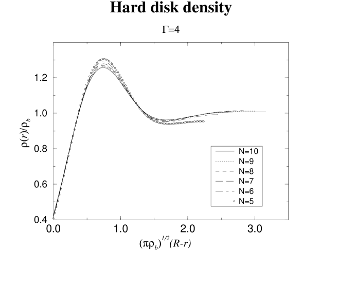
Figure 1: Density profile in the hard disk case for several values of $N$ at $\Gamma=4$. The boundary of the disk is taken as origin.

To investigate the rate of convergence of the whole profile as measured from the boundary to the thermodynamic value we can investigate the contact theorem [CFG80]. This expresses the thermodynamic pressure in terms of the density at contact with the wall, and the potential drop across the interface (which in turn is proportional to the first moment of the density profile). Explicitly the contact theorem states

$$\Big{(}1-{\Gamma\over 4}\Big{)}\rho_{b}=\rho(0)-2\pi\rho_{b}\Gamma\int_{0}^{\infty}x(\rho(x)-\rho_{b})\,dx$$ (3.16)

where we stress again that the density is measured from the boundary.

Much to our initial surprise, the convergence of the r.h.s. to the l.h.s. for the finite $N$ data is very slow. For 10 particles the error is of order $30\%$. Further investigation reveals that this is not special to the coupling $\Gamma=4$. At $\Gamma=2$ we have the analytic expression [Jan81]

$$\rho_{(1)}(r)={1\over 2\pi}\sum_{j=1}^{N}{(R-r)^{2j-2}e^{-\pi(R-r)^{2}}\over\int_{0}^{R}s^{2j-1}e^{-\pi s^{2}}\,ds},\quad 0\leq r\leq R$$

where $r$ is measured from the boundary and the background density is taken to equal unity. Choosing $N=10$ and substituting in (3.16) again gives an error of order $30\%$. Indeed choosing $N=500$ still gives an error of order $3\%$.

In fact the slow convergence of (3.16) can be understood analytically by making use of a sum rule for the OCP applicable for the finite disk [CFG80]. This sum rule reads

$$\rho_{(1)}(0)-\Big{(}1-{\Gamma\over 4}\Big{)}\rho_{b}=-{\Gamma\rho_{b}^{2}\pi^{2}\over N}\int_{0}^{R}r^{3}\Big{(}\rho_{(1)}(R-r)-\rho_{b}\Big{)}\,dr$$ (3.17)

where $\rho_{(1)}(r)$ is measured inward from the boundary. Noting that charge neutrality requires

$$\int_{0}^{R}r\Big{(}\rho_{(1)}(R-r)-\rho_{b}\Big{)}\,dr=\int_{0}^{R}(R-r)\Big{(}\rho_{(1)}(r)-\rho_{b}\Big{)}\,dr$$

we can write

$$-{\Gamma\rho_{b}^{2}\pi^{2}\over N}\int_{0}^{R}r^{3}\Big{(}\rho_{(1)}(R-r)-\rho_{b}\Big{)}\,dr$$

$$=-{\Gamma\rho_{b}^{2}\pi^{2}\over N}\int_{0}^{R}(R-r)^{3}\Big{(}\rho_{(1)}(r)-\rho_{b}\Big{)}\,dr$$

$$=-{\Gamma\rho_{b}^{2}\pi^{2}\over N}\int_{0}^{R}(-2rR^{2}+3r^{2}R-r^{3})\Big{(}\rho_{(1)}(r)-\rho_{b}\Big{)}\,dr$$

$$=2\Gamma\rho_{b}\pi\int_{0}^{R}r\Big{(}\rho_{(1)}(r)-\rho_{b}\Big{)}\,dr-{3\Gamma(\rho_{b}\pi)^{3/2}\over N^{1/2}}\int_{0}^{R}r^{2}\Big{(}\rho_{(1)}(r)-\rho_{b}\Big{)}\,dr$$

$$\quad+{\Gamma\rho_{b}^{2}\pi^{2}\over N}\int_{0}^{R}r^{3}\Big{(}\rho_{(1)}(r)-\rho_{b})\,dr$$

This shows that the finite size corrections to the r.h.s. of (3.17) are proportional to $N^{-1/2}$, thus explaining our empirical observation.

Two-point function

At $\Gamma=2$ and in the thermodynamic limit the two-particle distribution function has the exact evaluation [Jan81]

$$\rho_{(2)}({0},\vec{r})=\rho_{b}^{2}\Big{(}1-e^{-\pi\rho_{b}|\vec{r}|^{2}}\Big{)}.$$

This is a monotonic function, with the corresponding truncated distribution $\rho_{(2)}^{T}({0},\vec{r}):=\rho_{(2)}({0},\vec{r})-\rho_{(1)}({0})\rho_{(1)}({\vec{r}\,})$ exhibiting Gaussian decay to zero. There is evidence, both analytic and numerical [Jan81, CLWH82] which suggests that for $\Gamma>2$ the two-particle distribution exhibits oscillations. At $\Gamma=4$ this feature has already been observed in the exact finite $N$ calculation of $\rho_{(2)}({0},\vec{r})$ by Samaj et al. [SPK94]. Furthermore, this feature should become more pronounced as $\Gamma$ increases. This is indeed what we observe when plotting our results for $\Gamma=4$ and $\Gamma=6$ on the same graph (see Figure 2).

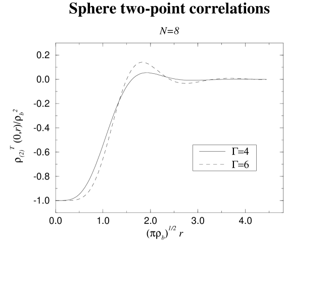
Figure 2: Two-point correlation in the sphere case for $N=8$ particles at $\Gamma=4$ and $\Gamma=6$.

The fact that the 2dOCP is a Coulomb system in its conductive phase implies that in the bulk the second moment of the truncated distribution obeys the Stillinger-Lovett sum rule

$$\int_{{\mathbf{R}}^{2}}\vec{r}\,{}^{2}\rho_{(2)}^{T}(0,\vec{r})\,d\vec{r}=-{2\over\pi\Gamma}.$$ (3.18)

For the hard disk in the finite system we can compute

$$\int_{|\vec{r}|<R}\vec{r}\,{}^{2}\rho_{(2)}^{T}({0},\vec{r})\,d\vec{r}$$ (3.19)

and compare it with the universal value given by (3.18). At $\Gamma=4$ and with $N=9$ we find agreement with the universal value to within $2\%$. In fact, analogous to the integral in (3.17), the integral (3.19) can be evaluated exactly and the terms which differ from $-2/\pi\Gamma$ read off. In the hard wall case we find

$$\int_{|\vec{r}|<R}{\vec{r}\,}^{2}\rho_{(2)}^{T}(\vec{0},\vec{r})\,d\vec{r}=-{2\over\pi\Gamma}\bigg{(}\rho_{(1)}(0)/\rho_{b}+N\rho_{(2)}^{T}(0,R)/\rho_{b}^{2}\bigg{)},$$ (3.20)

while in the soft wall case the same expression results except that the boundary term $N\rho_{(2)}^{T}(0,R)/\rho_{b}^{2}$ is no longer present on the r.h.s., while on the l.h.s. the integral is over ${\mathbf{R}}^{2}$.

We see from (3.20) that the deviation in the finite system from the bulk value (3.18) is determined by

$$-{2\over\pi\Gamma}\Big{(}(\rho_{(1)}(0)-\rho_{b})/\rho_{b}+N\rho_{(2)}^{T}(0,R)/\rho_{b}^{2}\Big{)},$$

and thus consists of a bulk and surface contribution.

4 New sum rules

In this section we present the derivation of the sum rule (3.20) and its generalization to multicomponent Coulomb systems. First we show that the sum rule can be derived within the formalism of Section 2, then we present a more general derivation of the sum rule.

4.1 The case $\Gamma$ even

The formalism presented in Section 2 is valid only if $\Gamma$ is an even integer. Within this formalism we can use the expressions (2.31) and (2.32) for the two-point correlation functions (and its generalizations to higher $\Gamma$) to compute the second moment

$$\int_{\Lambda}{\vec{r}\,}^{2}\rho_{(2)}^{T}(0,{\vec{r}\,})\,d{\vec{r}\,}\,,$$ (4.1)

where $\Lambda$ is a disk of radius $R$ (hard disk) or ${\mathbf{R}}^{2}$ (soft disk). For example in the hard disk case with $\Gamma=4$, for each term in the sum (2.31) the integral (4.1) gives an incomplete gamma function $\gamma(\mu_{j}+2,2N)$. Then we use the recurrence relation

$$\gamma(\mu_{j}+2,2N)=(\mu_{j}+1)\gamma(\mu_{j}+1,2N)-e^{-2N}(2N)^{\mu_{j}+1}$$ (4.2)

to split the expression in two. The first term is proportional to $\rho_{(1)}(0)$ while the second is proportional to $\rho_{(2)}(0,R)$. The sum rule (3.20) follows from that.

The calculation can be easily generalized to any even $\Gamma$. In the soft disk case since the incomplete gamma functions are replaced by complete gamma functions the recurrence relation (4.2) does not have a second term on the r.h.s., therefore there is no surface contribution proportional to $\rho_{(2)}^{T}(0,R)$ in the sum rule.

4.2 General case

In fact a more general derivation of this sum rule, valid for any value of the coupling constant, can be obtained by studying the variations of the density as a function of the size of the disk.

Let us consider the general case of a multicomponent jellium in $\nu$ dimensions confined in a spherical domain $\Lambda$ of radius $R$ and volume $V=\Omega_{\nu}R^{\nu}/\nu$ with $\Omega_{\nu}=2\pi^{\nu/2}/\Gamma(\nu/2)$. The system is composed of $s$ different species with charges $(e_{\alpha})_{\alpha\in\{1,\dots,s\}}$ and there are $N_{\alpha}$ particles of the species $\alpha$. Let $N=\sum_{\alpha}N_{\alpha}$ be the total number of particles and let us define the average density of the species $\alpha$, $\rho_{\alpha}=N_{\alpha}/V$ and the total average density $\rho=N/V$. As in the preceding sections $\rho_{b}$ is the background number density and let $e_{b}$ be its charge so that the background charge density is $e_{b}\rho_{b}$. For convenience let us define the “number of particles of the background” by $N_{b}=\rho_{b}V$. In general the Coulomb potential is

$$\Phi({\vec{r}\,})=\cases{-\ln r,&if $\nu=2$\cr\displaystyle\frac{r^{2-\nu}}{\nu-2},&otherwise,}$$ (4.3)

and the Coulomb force is

$${\vec{F}}({\vec{r}\,})=-\nabla\Phi({\vec{r}\,})=\frac{{\vec{r}\,}}{r^{\nu}}\,.$$ (4.4)

The Hamiltonian of the Coulomb system is

$$U=\frac{1}{2}\sum_{i\neq j}e_{\alpha_{i}}e_{\alpha_{j}}\Phi({\vec{r}\,}_{i}-{\vec{r}\,}_{j})+e_{b}\rho_{b}\sum_{i=1}^{N}e_{\alpha_{i}}\int_{\Lambda}d{\vec{r}\,}\Phi({\vec{r}\,}_{i}-{\vec{r}\,})+\frac{e_{b}^{2}\rho_{b}^{2}}{2}\int_{\Lambda^{2}}d{\vec{r}\,}d{\vec{r}\,}^{\prime}\Phi({\vec{r}\,}-{\vec{r}\,}^{\prime})\,.$$ (4.5)

We shall consider the correlation functions in the canonical ensemble

$$\rho_{\alpha_{1}\dots\alpha_{n}}^{(n)}({\vec{r}\,}_{1},\dots,{\vec{r}\,}_{n})=\left<\sum_{i_{1}=1}^{N_{\alpha_{1}}}\cdots\sum_{i_{n}=1}^{N_{\alpha_{n}}}\delta({\vec{r}\,}_{1}-{\vec{r}\,}_{\alpha_{1},i_{1}})\cdots\delta({\vec{r}\,}_{n}-{\vec{r}\,}_{\alpha_{n},i_{n}})\right>\,.$$ (4.6)

The $\left<\cdots\right>$ is the average in the canonical ensemble and in the preceding sums if some $\alpha_{a}=\alpha_{b}$ we exclude the term $i_{a}=i_{b}$ as usual.

In three dimensions in order to have a well defined thermodynamic limit we shall restrict ourselves to the case where all electric charges $e_{\alpha}$ have the same sign and the background carries a opposite neutralizing charge. In two dimensions we can also consider systems with charges of different signs and eventually without background ($\rho_{b}=0$) if the coupling contants $|\beta e_{\alpha}e_{\gamma}|<2$ for all pair of charges $(e_{\alpha},\,e_{\gamma})$ of different signs.

4.2.1 Contact theorem sum rule

The derivation of the sum rule for the second moment of the two-point correlation function is similar to that of the contact theorem for a spherical domain [CFG80]. Let us first show here the generalization of this contact theorem for the multicomponent jellium. We consider the canonical partition function (times $N!$)

$${\cal Q}=\int_{\Lambda^{N}}d{\vec{r}\,}^{N}\exp(-\beta U)\,,$$ (4.7)

as a function of the volume $V$. We shall compute the thermodynamical pressure $p^{(\theta)}=\partial\log{\cal Q}/\partial V$ in two different ways. The derivative is done at fixed number of particles and fixed $N_{b}$. In general using the scaling ${\vec{r}\,}=V^{1/\nu}\tilde{{\vec{r}\,}}$ we have

$$\beta p^{(\theta)}=\frac{\partial\ln{\cal Q}}{\partial V}=\rho-\frac{\beta V^{N}}{{\cal Q}}\int_{\tilde{\Lambda}^{N}}d\tilde{{\vec{r}\,}}^{N}\frac{\partial U(V^{1/\nu}\tilde{{\vec{r}\,}})}{\partial V}e^{-\beta U}\,,$$ (4.8)

where $\tilde{\Lambda}$ is a sphere of volume 1.

A first way to compute the derivative of $U$ is by using the general formula

$$\frac{\partial\Phi(V^{1/\nu}\tilde{{\vec{r}\,}})}{\partial V}=-\frac{1}{\nu V}\,{\vec{r}\,}\cdot{\vec{F}}({\vec{r}\,})\,.$$ (4.9)

This gives, together with the definition (4.5) of $U$,

$$\beta p^{(\theta)} =\rho+\displaystyle\frac{\beta}{\nu V} \left[\int_{\Lambda^{2}}d{\vec{r}\,}d{\vec{r}\,}^{\prime}{\vec{r}\,}\cdot{\vec{F}}({\vec{r}\,}-{\vec{r}\,}^{\prime})\sum_{\alpha,\alpha^{\prime}}e_{\alpha}e_{\alpha^{\prime}}\rho_{\alpha\alpha^{\prime}}^{(2)}({\vec{r}\,},{\vec{r}\,}^{\prime})\right.$$ (4.10)

$$+e_{b}\rho_{b}\int_{\Lambda^{2}}d{\vec{r}\,}d{\vec{r}\,}^{\prime}({\vec{r}\,}-{\vec{r}\,}^{\prime})\cdot{\vec{F}}({\vec{r}\,}-{\vec{r}\,}^{\prime})\sum_{\alpha}e_{\alpha}\rho_{\alpha}^{(1)}({\vec{r}\,}^{\prime})$$

$$\left.+\frac{1}{2}e_{b}^{2}\rho_{b}^{2}\int_{\Lambda^{2}}d{\vec{r}\,}d{\vec{r}\,}^{\prime}({\vec{r}\,}-{\vec{r}\,}^{\prime})\cdot{\vec{F}}({\vec{r}\,}-{\vec{r}\,}^{\prime})\right]\,.$$

We can transform the preceding expression by using the first equation of the BGY hierarchy

$$k_{B}T\nabla\rho_{\alpha}({\vec{r}\,})=e_{\alpha}\rho_{b}e_{b}\int_{\Lambda}d{\vec{r}\,}^{\prime}\,{\vec{F}}({\vec{r}\,}-{\vec{r}\,}^{\prime})\rho_{\alpha}^{(1)}({\vec{r}\,})+\int_{\Lambda}d{\vec{r}\,}^{\prime}\sum_{\alpha^{\prime}}e_{\alpha}e_{\alpha^{\prime}}{\vec{F}}({\vec{r}\,}-{\vec{r}\,}^{\prime})\rho_{\alpha\alpha^{\prime}}^{(2)}({\vec{r}\,},{\vec{r}\,})\,.$$ (4.11)

The r.h.s of (4.11) appears in the first and second lines of (4.10). Replacing it by the l.h.s of (4.11) we find

$$\beta p^{(\theta)} =\rho+\displaystyle\frac{\beta}{\nu V} \left[k_{B}T\int_{\Lambda}d{\vec{r}\,}\sum_{\alpha}{\vec{r}\,}\cdot\nabla\rho_{\alpha}^{(1)}({\vec{r}\,})\right.$$ (4.12)

$$-e_{b}\rho_{b}\int_{\Lambda^{2}}d{\vec{r}\,}d{\vec{r}\,}^{\prime}{\vec{r}\,}^{\prime}\cdot{\vec{F}}({\vec{r}\,}-{\vec{r}\,}^{\prime})\sum_{\alpha}e_{\alpha}\rho_{\alpha}^{(1)}({\vec{r}\,})$$

$$\left.+\frac{1}{2}\rho_{b}^{2}e_{b}^{2}\int_{\Lambda^{2}}d{\vec{r}\,}d{\vec{r}\,}^{\prime}\,({\vec{r}\,}-{\vec{r}\,}^{\prime})\cdot{\vec{F}}({\vec{r}\,}-{\vec{r}\,}^{\prime})\right]\,.$$

The first term of the r.h.s of the preceding equation can be computed by integration by parts while the others can be computed using the definition (4.4) of the Coulomb force ${\vec{F}}$ and Newton’s theorem. This yields the following expression for the thermodynamical pressure

$$\beta p^{(\theta)} = \sum_{\alpha}\rho_{\alpha}^{(1)}(R)+\beta e_{b}\rho_{b}R^{2-\nu}\left(\sum_{\alpha}e_{\alpha}\frac{N_{\alpha}}{2}+e_{b}\frac{N_{b}}{\nu+2}\right)$$ (4.13)

$$-\frac{\beta\rho_{b}e_{b}}{2R^{\nu}}\int_{\Lambda}d{\vec{r}\,}\,r^{2}\sum_{\alpha}e_{\alpha}\rho_{\alpha}^{(1)}({\vec{r}\,})\,.$$

The other way to compute the thermodynamical pressure is to use the actual scaling properties of the Coulomb potential $\Phi$,

$$\frac{\partial\Phi(V^{1/\nu}\tilde{{\vec{r}\,}})}{\partial V}=\cases{\displaystyle-\frac{1}{2V},&if $\nu=2$\cr\displaystyle\frac{2-\nu}{\nu V}\,\Phi({\vec{r}\,}),&otherwise.}$$ (4.14)

Substituting this expression in (4.8) gives

$$\beta p^{(\theta)}=\rho+{\beta\delta_{\nu,2}\over 4}\left(\frac{Q^{2}}{V}-\sum_{\alpha}e_{\alpha}^{2}\rho_{\alpha}\right)+\frac{\nu-2}{\nu V}\beta\left<U\right>\,,$$ (4.15)

where $Q=\sum_{\alpha}e_{\alpha}N_{\alpha}+e_{b}N_{b}$ is the total charge of the system.

Equating the two expressions (4.13) and (4.15) of the thermodynamic pressure we find the generalization of the contact theorem

$$\sum_{\alpha}\rho_{\alpha}^{(1)}(R)+\frac{\beta e_{b}\rho_{b}}{2R^{\nu-2}}Q-\frac{\beta e_{b}\rho_{b}}{2R^{\nu}}\int_{\Lambda}d{\vec{r}\,}\,r^{2}q({\vec{r}\,})$$ (4.16)

$$=\rho+\delta_{\nu,2}\frac{\beta}{4}\left(\frac{Q^{2}}{V}-\sum_{\alpha}e_{\alpha}^{2}\rho_{\alpha}\right)+\frac{\nu-2}{\nu V}\beta\left<U\right>$$

where $q({\vec{r}\,})=\sum_{\alpha}e_{\alpha}\rho_{\alpha}^{(1)}({\vec{r}\,})+e_{b}\rho_{b}$ is the local charge density.

4.2.2 Density-charge correlation second moment sum rule

Similar calculations lead to the second moment sum rule for the density-charge truncated correlation function $\sum_{\beta}e_{\beta}\rho_{\alpha\beta}^{(2)T}(0,{\vec{r}\,})$. Here we consider the quantity

$${\cal Q}_{\alpha}=\int_{\Lambda^{N}}d{\vec{r}\,}^{N}e^{-\beta U}\sum_{i=1}^{N_{\alpha}}\delta({\vec{r}\,}_{i,\alpha})\,,$$ (4.17)

as a function of the volume $V$. Note that the density of the species $\alpha$ at the center of the spherical domain is $\rho_{\alpha}^{(1)}(0)={\cal Q}_{\alpha}/{\cal Q}$. Like in the preceding section we want to compute by two different ways the quantity ${\cal Q}^{-1}\partial{\cal Q}_{\alpha}/\partial V$. Using the same scaling argument as before we have

$$\frac{1}{{\cal Q}}\frac{\partial{\cal Q}_{\alpha}}{\partial V}=\frac{N-1}{V}\rho_{\alpha}^{(1)}(0)-\beta\frac{V^{N}}{{\cal Q}}\int_{\tilde{\Lambda}^{N}}d\tilde{r}^{N}\sum_{i=1}^{N_{\alpha}}\delta(V^{1/\nu}\tilde{{\vec{r}\,}}_{i,\alpha})\,\frac{\partial U(V^{1/\nu}\tilde{{\vec{r}\,}})}{\partial V}\,e^{-\beta U}\,.$$ (4.18)

Using eq. (4.9) and the definition (4.5) of the Hamiltonian $U$ we find

$$\frac{1}{{\cal Q}}\frac{\partial{\cal Q}_{\alpha}}{\partial V} = \frac{N-1}{V}\rho_{\alpha}^{(1)}(0)$$ (4.19)

$$+\frac{\beta}{\nu V}\left[\int_{\Lambda^{2}}d{\vec{r}\,}d{\vec{r}\,}^{\prime}\,{\vec{r}\,}\cdot{\vec{F}}({\vec{r}\,}-{\vec{r}\,}^{\prime})\sum_{\beta,\gamma}e_{\beta}e_{\gamma}\rho_{\alpha\beta\gamma}^{(3)}(0,{\vec{r}\,},{\vec{r}\,}^{\prime})\right.$$

$$+\int_{\Lambda}{\vec{r}\,}\cdot{\vec{F}}({\vec{r}\,})e_{\alpha}\sum_{\beta}e_{\beta}\rho_{\alpha\beta}^{(2)}(0,{\vec{r}\,})$$

$$+e_{b}\rho_{b}\int_{\Lambda^{2}}d{\vec{r}\,}d{\vec{r}\,}^{\prime}\sum_{\beta}e_{\beta}\rho_{\alpha\beta}^{(2)}(0,{\vec{r}\,})\,{\vec{r}\,}\cdot{\vec{F}}({\vec{r}\,}-{\vec{r}\,}^{\prime})$$

$$-e_{b}\rho_{b}\int_{\Lambda^{2}}d{\vec{r}\,}d{\vec{r}\,}^{\prime}{\vec{r}\,}^{\prime}\cdot{\vec{F}}({\vec{r}\,}-{\vec{r}\,}^{\prime})\sum_{\beta}e_{\beta}\rho_{\alpha\beta}^{(2)}(0,{\vec{r}\,})$$

$$+e_{b}\rho_{b}\int_{\Lambda}d{\vec{r}\,}\,{\vec{r}\,}\cdot{\vec{F}}({\vec{r}\,})e_{\alpha}\rho_{\alpha}^{(1)}(0)$$

$$\left.+\frac{1}{2}e_{b}^{2}\rho_{b}^{2}\int_{\Lambda^{2}}d{\vec{r}\,}d{\vec{r}\,}^{\prime}\,({\vec{r}\,}-{\vec{r}\,}^{\prime})\cdot{\vec{F}}({\vec{r}\,}-{\vec{r}\,}^{\prime})\rho_{\alpha}^{(1)}(0)\right]$$

Using the second BGY equation

$$k_{B}T\nabla_{\vec{r}\,}\rho_{\alpha\beta}^{(2)}(0,{\vec{r}\,}) = e_{\beta}e_{b}\rho_{b}\int_{\Lambda}d{\vec{r}\,}^{\prime}\,{\vec{F}}({\vec{r}\,}-{\vec{r}\,}^{\prime})\rho_{\alpha\beta}^{(2)}(0,{\vec{r}\,})$$ (4.20)

$$+e_{\beta}e_{\alpha}{\vec{F}}({\vec{r}\,})\rho_{\alpha\beta}^{(2)}(0,{\vec{r}\,})$$

$$+\int_{\Lambda}d{\vec{r}\,}^{\prime}\,{\vec{F}}({\vec{r}\,}-{\vec{r}\,}^{\prime})\sum_{\gamma}e_{\beta}e_{\gamma}\rho_{\alpha\beta\gamma}^{(3)}(0,{\vec{r}\,},{\vec{r}\,}^{\prime})\,,$$

and then integration by parts

$$\sum_{\beta}\int_{\Lambda}{\vec{r}\,}\cdot\nabla_{\vec{r}\,}\rho_{\alpha\beta}^{(2)}(0,{\vec{r}\,})=\nu V\sum_{\beta}\rho_{\alpha\beta}^{(2)}(0,R)-\nu(N-1)\rho_{\alpha}^{(1)}(0)\,,$$ (4.21)

we can arrange expression (4.19) to find, after computing explicitly the integrals involving ${\vec{F}}$ using Newton’s theorem,

$$\frac{1}{{\cal Q}}\frac{\partial{\cal Q}_{\alpha}}{\partial V} = \sum_{\beta}\rho_{\alpha\beta}^{(2)}(0,R)-\frac{\beta e_{b}\rho_{b}}{2R^{\nu}}\int_{\Lambda}d{\vec{r}\,}\,r^{2}\sum_{\beta}e_{\beta}\rho_{\alpha\beta}^{(2)}(0,{\vec{r}\,})$$ (4.22)

$$+\frac{\beta e_{b}\rho_{b}}{2R^{\nu-2}}\rho_{\alpha}^{(1)}(0)\left[\sum_{\beta}e_{\beta}N_{\beta}+\frac{e_{b}N_{b}}{\nu+2}\right]\,.$$

The second way for computing ${\cal Q}^{-1}\partial{\cal Q}_{\alpha}/\partial V$ is by using directly equation (4.14) into equation (4.18). This gives,

$$\frac{1}{{\cal Q}}\frac{\partial{\cal Q}_{\alpha}}{\partial V} = \frac{N-1}{V}\rho_{\alpha}^{(1)}(0)+\frac{\beta}{4}\delta_{\nu,2}\left[\frac{Q^{2}}{V}-\sum_{\beta}e_{\beta}^{2}N_{\beta}\right]\rho_{\alpha}^{(1)}(0)$$ (4.23)

$$+\frac{\nu-2}{\nu V}\beta\left<U\hat{\rho}_{\alpha}^{(1)}(0)\right>\,,$$

where $\hat{\rho}_{\alpha}^{(1)}(0)=\sum_{i=1}^{N_{\alpha}}\delta({\vec{r}\,}_{i,\alpha})$ is the microscopic density of $\alpha$-particles at the center of the domain $\Lambda$.

Comparing the two expressions (4.22) and (4.23) of ${\cal Q}^{-1}\partial{\cal Q}_{\alpha}/\partial V$ gives a sum rule for the second moment of the density of $\alpha$ particles-electric charge correlation function. The sum rule takes a nice form by considering the truncated correlation function and making use of the contact sum rule (4.16),

$$\frac{\beta e_{b}\rho_{b}\Omega_{\nu}}{2\nu}\int_{\Lambda}d{\vec{r}\,}\,r^{2}\sum_{\beta}e_{\beta}\rho_{\alpha\beta}^{(2)T}(0,{\vec{r}\,}) = \rho_{\alpha}^{(1)}(0)+\frac{\Omega_{\nu}}{\nu}R^{\nu}\sum_{\beta}\rho_{\alpha\beta}^{(2)T}(0,R)$$ (4.24)

$$+\frac{2-\nu}{\nu}\,\beta\left<U\hat{\rho}_{\alpha}^{(1)}(0)\right>^{T}\,.$$

In the case of the two-dimensional OCP ($\nu=2$, $s=1$ and $e_{b}=-e_{1}$) this is exactly the sum rule (3.20) announced in the preceding section

$$\int_{|\vec{r}|<R}{\vec{r}\,}^{2}\rho_{(2)}^{T}(\vec{0},\vec{r})\,d\vec{r}=-{2\over\pi\Gamma}\bigg{(}\rho_{(1)}(0)/\rho_{b}+N\rho_{(2)}^{T}(0,R)/\rho_{b}^{2}\bigg{)}\,.$$ (3.20)

The sum rule (4.24) is in fact a series of $s$ sum rules for the density-charge correlation function $\sum_{\beta}e_{\beta}\rho^{(2)T}_{\alpha\beta}(0,{\vec{r}\,})$ for each species $\alpha$. By taking the sum of these sum rules with the factors $e_{\alpha}$, we find a sum rule for the charge-charge truncated correlation function $S(0,{\vec{r}\,})=\sum_{\alpha,\beta}e_{\alpha}e_{\beta}\rho^{(2)T}_{\alpha\beta}(0,{\vec{r}\,})$,

$$\frac{\beta e_{b}\rho_{b}\Omega_{\nu}}{2\nu}\int_{\Lambda}d{\vec{r}\,}\,r^{2}S(0,{\vec{r}\,}) = \sum_{\alpha}e_{\alpha}\rho_{\alpha}^{(1)}(0)+\frac{\Omega_{\nu}}{\nu}R^{\nu}\sum_{\alpha,\beta}e_{\alpha}\rho_{\alpha\beta}^{(2)T}(0,R)$$ (4.25)

$$+\frac{2-\nu}{\nu}\,\beta\left<U\sum_{\alpha}e_{\alpha}\hat{\rho}_{\alpha}^{(1)}(0)\right>^{T}\,.$$

4.2.3 Thermodynamic limit of the sum rules

Canonical ensemble

In order to study the relationship between sum rules (4.24) and (4.25) and the Stillinger–Lovett sum rule, we need to know the behavior of the correlation functions as they approach the thermodynamic limit. This behavior is different depending on the ensemble used. In this section we continue to work in the canonical ensemble.

In general we shall suppose that in the thermodynamic limit the system is in a fluid and conducting phase. In this case the density becomes uniform in the thermodynamic limit $\rho_{\alpha}^{(1)}(0)\to\rho_{\alpha}$ and

$$\left<\hat{\rho}_{\alpha}^{(1)}(0)U\right>^{T}\to\left<\rho_{\alpha}U\right>^{T}=0\,,$$ (4.26)

because in the canonical ensemble the density does not fluctuate.

Let us first consider the case of a multicomponent Coulomb system without background (in two dimensions with small Coulomb couplings). In that case equation (4.24) becomes

$$\rho_{\alpha}^{(1)}(0)+\frac{\Omega_{\nu}}{\nu}R^{\nu}\sum_{\beta}\rho_{\alpha\beta}^{(2)T}(0,R)=0\,.$$ (4.27)

This equation (4.27) give us the behavior of the correlation functions as they approach the thermodynamic limit

$$\sum_{\gamma}\rho_{\alpha\gamma}^{(2)T}(0,R)\sim-\rho\rho_{\alpha}/N\,.$$ (4.28)

This is a generalization of an already known result concerning the existence of $1/N$ tails for the correlation functions of one component fluids with short range forces [LP61]. However, for a neutral system taking the sum of equations (4.28) with the coefficients $e_{\alpha}$ show that the charge-total density correlation does not have $1/N$ tails,

$$R^{\nu}\sum_{\alpha\gamma}e_{\alpha}\rho_{\alpha\gamma}^{(2)T}(0,R)\to 0\,,$$ (4.29)

It is likely that a similar behavior exists in the general case ($\rho_{b}\neq 0$, $\nu=2,3$), so it would be difficult to derive from (4.24) partial sum rules for the density-charge correlations in the thermodynamic limit because with the $1/N$ tails, one cannot commute the thermodynamic limit with the integration over the space. However, one can conjecture that although the density-density correlations have $1/N$ tails, in the conductive phase the total density-charge correlations do not have these tails as it is in the case when $\rho_{b}=0$. If this is true, and assuming that the convergence of the charge-charge correlation function is uniform (in order to commute the thermodynamic limit with the integration over the space), one can recover the Stillinger–Lovett sum rule from the sum rule (4.25) for finite systems,

$$\frac{\beta\Omega_{\nu}}{2\nu}\int_{{\mathbf{R}}^{\nu}}d{\vec{r}\,}r^{2}S(0,{\vec{r}\,})=-1\,.$$ (4.30)

The fact that we recover the Stillinger–Lovett sum rule is of course not a proof of our conjecture, but at least it show that our conjecture is not in contradiction with well known results.

Grand canonical ensemble

For systems with short range forces the correlations functions do not have $1/N$ tails in the grand canonical ensemble as they approach the thermodynamic limit [LP61]. We will show that this is also the case for two-dimensional Coulomb systems with small couplings when there is no charged background and assuming this is also the case in general for a multicomponent jellium we will discuss the thermodynamic limit of the partial sum rules.

The partial sum rules (4.24) obtained before are different in the grand canonical ensemble. The grand canonical ensemble is parametrized by the background density $\rho_{b}$ and $s-1$ fugacities $\{z_{\gamma}\}$ used to fix $s-1$ average densities $\rho_{\gamma}$, the remaining density fixed by electroneutrality. The grand canonical version of the sum rules (4.24) can be obtained in a straightforward manner by adapting the calculations of the last section. However special care should be taken because of the fluctuation of the average densities in the grand canonical ensemble. These fluctuations add some extra terms to sum rule (4.24),

$$\frac{\beta e_{b}\rho_{b}\Omega_{\nu}}{2\nu}\int_{\Lambda}d{\vec{r}\,}\,r^{2}\sum_{\beta}e_{\beta}\rho_{\alpha\beta}^{(2)T}(0,{\vec{r}\,}) = \left<\hat{\rho}_{\alpha}^{(1)}(0)\right>+\frac{\Omega_{\nu}}{\nu}R^{\nu}\sum_{\beta}\rho_{\alpha\beta}^{(2)T}(0,R)$$ (4.31)

$$-\left<N\hat{\rho}^{(1)}_{\alpha}(0)\right>^{T}+\frac{2-\nu}{\nu}\,\beta\left<U\hat{\rho}_{\alpha}^{(1)}(0)\right>^{T}$$

$$+\delta_{\nu,2}\left<\sum_{\gamma}\frac{\beta e_{\gamma}^{2}}{4}N_{\gamma}\hat{\rho}_{\alpha}^{(1)}(0)\right>^{T}\,.$$

To proceed with the discussion of the thermodynamic limit of this sum rule, we need to use a relation that will allow us to simplify the terms on the r.h.s. of equation (4.31) in the thermodynamic limit. This relation reads for $\nu=2$ or 3,

$$\rho_{\alpha}-\left<N\rho_{\alpha}\right>^{T}+\frac{2-\nu}{\nu}\,\beta\left<U\rho_{\alpha}\right>^{T}+\delta_{\nu,2}\left<\sum_{\gamma}\frac{\beta e_{\gamma}^{2}}{4}N_{\gamma}\rho_{\alpha}\right>^{T}=\rho_{b}\frac{\partial\rho_{\alpha}}{\partial\rho_{b}}\,.$$ (4.32)

This relation is a consequence of the scaling properties of the Coulomb potential. To prove it, let us consider the thermodynamic grand canonical pressure

$$\beta\tilde{p}(\beta,\{z_{\gamma}\},\rho_{b})=\lim_{V\to\infty}V^{-1}\ln\Xi(\beta,\{z_{\gamma}\},\rho_{b},V)\,,$$ (4.33)

where $\Xi$ is the grand canonical partition function. Using the scaling properties of the Coulomb potential we have for $\nu=3$

$$\beta\tilde{p}(\beta,\{z_{\alpha}\},\rho_{b})=\lambda^{4}\beta\tilde{p}(\lambda\beta,\{\lambda^{-3/2}z_{\alpha}\},\lambda^{-3}\rho_{b})\,,$$ (4.34)

and for $\nu=2$,

$$\beta\tilde{p}(\beta,\{z_{\alpha}\},\rho_{b})=\beta\tilde{p}(\beta,\{\lambda^{-2(1-(\beta e_{\alpha}^{2}/4))}z_{\alpha}\},\lambda^{-2}\rho_{b})\,,$$ (4.35)

for any positive number $\lambda$. Taking the derivative of these relations with respect to $\lambda$, then putting $\lambda=1$ and using the usual thermodynamic relations yields for $\nu=3$,

$$\tilde{p}=\frac{1}{3}\left<H\right>+\frac{1}{2\beta}\rho-\rho_{b}\frac{\partial\tilde{p}}{\partial\rho_{b}}=\frac{1}{3}\left<U\right>+\frac{1}{\beta}\rho-\rho_{b}\frac{\partial\tilde{p}}{\partial\rho_{b}}\,,$$ (4.36)

and for $\nu=2$,

$$\beta\tilde{p}=\sum_{\alpha}\left(1-\frac{\beta e_{\alpha}^{2}}{4}\right)\rho_{\alpha}+\beta\rho_{b}\frac{\partial\tilde{p}}{\partial\rho_{b}}\,.$$ (4.37)

where $\left<H\right>$ is the total internal energy (including the kinetic term). The announced relation (4.32) follows from taking the derivative of (4.36) and (4.37) with respect to the fugacities.

As before let us consider first the case $\rho_{b}=0$ (in two dimensions for systems with small couplings). Then equation (4.31) together with equation (4.32) shows that the grand canonical total density-partial density correlation function does not exhibit any $1/N$ tails,

$$R^{\nu}\sum_{\alpha\gamma}\rho^{(2)T}_{\alpha\gamma}(0,R)\to 0\,.$$ (4.38)

Now if we suppose that in the general case ($\rho_{b}\neq 0$, $\nu=2,3$) this property still holds and that the density-charge correlation functions converge uniformly we recover the partial sum rules

$$\frac{\beta e_{b}\Omega_{\nu}}{2\nu}\int_{{\mathbf{R}}^{\nu}}d{\vec{r}\,}r^{2}\sum_{\gamma}e_{\gamma}\rho_{\alpha\gamma}^{(2)T}(0,{\vec{r}\,})=\frac{\partial\rho_{\alpha}}{\partial\rho_{b}}\,,$$ (4.39)

that have been previously derived by Suttorp and van Wonderen [SvW87] in the three dimensional case. These equations also hold for two-dimensional systems. One can recover the Stillinger–Lovett sum rule (4.30) by taking the sum of these equations (4.39) with the factors $e_{\alpha}$ and using electroneutrality. Notice that the condition (4.38) on the thermodynamic limit of the two-point correlation function when one of the points is in the boundary is different from the usual condition needed to prove the Stillinger–Lovett [MG83] that the correlation function of the infinite system should decay faster than $1/r^{\nu+2}$.

Notwithstanding the relation of the sum rules (4.24) and (4.31) with the Stillinger–Lovett sum rule (4.30), let us stress that for finite systems these sum rules are not screening sum rules like the Stillinger–Lovett sum rule since for finite systems the screening of external charges does not exists (because since the total electric charge is conserved, the excess of charge can not leak out to infinity like it does in infinite systems). From the derivation presented in the previous section it is clear that the new sum rules should be seen more as a second order contact theorem rather than a screening sum rule. Futhermore when there is no background ($\rho_{b}=0$) the relation with Stillinger–Lovett sum rule disappears because the term containing the second moment of the density-charge correlation vanishes.

5 Summary and conclusion

Expanding the power of the Vandermonde determinant that appears in the Boltzmann factor of the 2dOCP in terms of simple orthogonal polynomials we have been able to develop exact numerical solutions for values of the coupling constant $\Gamma=4$ and $\Gamma=6$ for finite systems up to 11 and 9 particles respectively for different kinds of geometry (sphere, soft and hard wall disk). With these solutions we have been able to test the prediction [JMP94] of universal logarithmic finite size corrections to the free energy (1.3). Studying the correlation functions has lead us to find a new sum rule (3.20) similar to the Stillinger–Lovett sum rule for finite systems. This sum rule can be derived within the formalism of section 2, but can also be generalized to higher dimension and multicomponent jellium systems (eq. (4.24)).

Further applications of the formalism presented here are the study of surface correlations which are expected to have a universal behavior at large distances [Jan95]. Also the formal expressions of the correlations functions (2.31) and (2.32) could eventually be used to find higher order sum rules or other general properties.

References

- [AJ81] A. Alastuey and B. Jancovici. On the two-dimensional one-component Coulomb plasma. J. Physique, 42:1–12, 1981.
- [Bar00] E.W. Barnes. The theory of the -function. Quart. J. Pure Appl. Math., 31:264–313, 1900.
- [Cai81] J.M. Caillol. J. Phys. Lett. (Paris), 42:L245, 1981.
- [CFG80] Ph. Choquard, P. Favre, and Ch. Gruber. On the equation of state of classical one-component systems with long-range forces. J. Stat. Phys., 23:405–442, 1980.
- [Cho81] Ph. Choquard. Helv. Phys. Acta, 54:332, 1981.
- [CLWH82] J.M. Caillol, D. Levesque, J.J. Weiss, and J.P. Hansen. J. Stat. Phys., 28:325, 1982.
- [Dun94] G.V. Dunne. Slater decomposition of Laughlin states. Int. J. Mod. Phys. B, 7:4783–4813, 1994.
- [FGIL94] F. Di Francesco, M. Gaudin, C. Itzykson, and F. Lesage. Laughlin’s wavefunctions, coulomb gases and expansions of the discriminant. Int. J. Mod. Phys. A, 9:4257, 1994.
- [Jan81] B. Jancovici. Exact results for the two-dimensional one-component plasma. Phys. Rev. Lett., 46:386–388, 1981.
- [Jan95] B. Jancovici. Classical Coulomb systems: screening and correlations revisited. J. Stat. Phys., 80:445–459, 1995.
- [JMP94] B. Jancovici, G. Manificat, and C. Pisani. Coulomb systems seen as critical systems: finite-size effects in two dimensions. J. Stat. Phys., 76:307–330, 1994.
- [JT98] B. Jancovici and G. Téllez. Two-dimensional Coulomb systems on a surface of constant negative curvature. J. Stat. Phys., 91:953, 1998.
- [JM83] S. Johannesen and D. Merlini. On the thermodynamics of two-dimensional jellium. J. Phys. A, 16:1449–1463, 1983.
- [Lau83] R.B. Laughlin. Anomalous quantum Hall effect: an incompressible quantum fluid with fractionally charge excitations. Phys. Rev. Lett., 50:1395–1398, 1983.
- [LP61] J. L. Lebowitz and J. K. Percus. Long-range correlations in a closed system with applications to nonuniform fluids. Phys. Rev.,122:1675 (1961)
- [Mar88] Ph. A. Martin. Sum rules in charged fluids. Rev. Mod. Phys., 60:1075–1127, 1988.
- [MG83] Ph. A. Martin and Ch. Gruber. A new proof of the Stillinger–Lovett complete shielding condition. J. Stat. Phys. 31:691, 1983.
- [SPK94] L. Samaj, J.K. Percus, and M. Kolesik. Two-dimensional one-component plasma at coupling : Numerical study of pair correlations. Phys. Rev. E, 49:5623–5627, 1994.
- [STW94] T. Scharf, J.-Y. Thibon and B.G. Wybourne. Powers of the Vandermonde determinant and the quantum Hall effect. J. Phys. A, 27:4211–4219, 1994.
- [SvW87] L. G. Suttorp and A. J. van Wonderen. Equilibrium properties of a multicomponent ionic mixture. Physica A, 145:577 (1987)