Critical behaviour of a spin-tube model in a magnetic field

Abstract

We show that the low-energy physics of the spin-tube model in presence of a critical magnetic field can be described by a broken SU(3) spin chain. Using the Lieb-Schultz-Mattis Theorem we characterize the possible magnetization plateaus and study the critical behavior in the region of transition between the plateaus $\langle S^{z}\rangle=1/2$ and $\langle S^{z}\rangle=3/2$ by means of renormalization group calculations performed on the bosonized effective continuum field theory. We show that in certain regions of the parameter space of the effective theory the system remains gapless, and we compute the spin-spin correlation functions in these regions. We also discuss the possibility of a plateau at $\langle S^{z}\rangle=1$, and show that although there exists in the continuum theory a term that might cause the appearance of a plateau there, such term is unlikely to be relevant. This conjecture is proved by DMRG techniques. The modifications of the three-leg ladder Hamiltonian that might show plateaus at $\langle S^{z}\rangle=1,5/6,7/6$ are discussed, and we give the expected form of correlation functions on the $\langle S^{z}\rangle=1$ plateau.

PACS numbers: 75.10.Jm, 75.30.Kz, 75.40.Gb
keywords: SU(3) spin-chain, renormalization group, magnetization plateaus, Density Matrix Renormalization Group

I Introduction

One-dimensional and quasi-one dimensional quantum spin systems have attracted much attention in recent years due to the large number of experimental realizations of such systems and the variety of theoretical techniques, both analytical and numerical, available to study the relevant models. Due to the presence of large quantum fluctuations in low dimensions, these systems present unusual properties such as a gap between a singlet ground state and excited non-singlet states. Examples include spin ladder systems in which a small number of one-dimensional spin-1/2 chains interact among themselves[1]. In this case, in a way very similar to the Haldane spin-S problem[2], it has been found that if the number of chains is even the system effectively behaves as an integer spin chain with a gap in the low-energy spectrum, while it remains massless for an odd number of chains. Some two-chain ladders which exhibit a gap are $SrCu_{2}O_{3}$[3] and $Cu_{2}(C_{5}H_{12}N_{2})_{2}Cl_{4}$[4], and an example of a gapless three-chain ladder is $Sr_{2}Cu_{3}O_{5}$[3]. Thus far we implicitly assumed that the boundary conditions in the transverse direction were open boundary conditions (OBC). These boundary conditions correspond to having all the chains lying in the same plane. This is the situation encountered in experimental systems such as $Sr_{2}Cu_{3}O_{5}$. In contrast with OBC, periodic boundary conditions (PBC) are frustrating for (2n+1) coupled chains. As a consequence all the spin excitations are gapped[5, 6] in the case of periodic boundary conditions. They are also gapped for 2n chains with PBC but the mechanism is related to singlet formation as in the OBC case and not frustration. The PBC could be achieved in an experimental system by having the coupled chains forming a cylinder instead of lying in a plane.

A richer behaviour emerges when these gapped or ungapped systems are placed in a magnetic field. Then it is possible for an integer spin chain to be gapless and a half-odd-integer spin chain to show a gap above the ground state for certain values of the field[7, 8, 9, 10]. This has been demonstrated by several methods such as bosonization [5, 11], perturbation theory[12] or density-matrix renormalization group method (DMRG)[13, 14, 15]. In particular, it has been shown that spin-1/2 chains and ladders with a gap undergo a continuous phase transition from a commensurate zero uniform magnetization phase to an incommensurate phase with non-zero magnetization[10], and the magnetization of the system can exhibit plateaus at certain non-zero values of the magnetic field[8, 16]. Further, a striking property of the quantum spin-chains in a uniform magnetic field pointing along the direction of the axial symmetry ($z$-direction), is the topological quantization of the magnetization under a changing of the magnetic field[7]. It was shown that starting from a generalized Lieb-Schultz-Mattis (LSM) theorem[17], that translationally invariant spin chains in an applied field can be gapful without breaking translational symmetry, only when the magnetization per spin, $m$, obeys $S-m=integer$, where $S$ is the maximum possible spin in each unit cell of the Hamiltonian. Such gapped phases correspond to plateaus at these quantized values of $m$. In Ref. [18] the behavior of the magnetization versus magnetic field has been investigated in details using DMRG techniques for three coupled spin 1/2 chains with both periodic and open boundary conditions. Plateaus have been obtained at $m=1/2$ and $m=3/2$ in agreement with Ref. [7]. Further, for the case of PBC a small plateau at $m=0$ was also obtained [9, 15, 18]. Finally, there seems to exist some weak evidence for a plateau at $m=1$ for PBC[18]. Strong coupling Low Energy Hamiltonians for these two systems were also derived in Ref. [18].

In this paper, we investigate a three-chain ladder with PBC (spin-tube) in presence of a uniform magnetic field by using bosonization and renormalization group techniques. We are concerned by the transition region between the magnetization plateaus at $m=1/2$ and $m=3/2$. Our analysis is based on the low-energy effective Hamiltonian (LEH) derived for strong coupling between the rungs[18]. We identify the LEH as an anisotropic SU(3) spin chain with symmetry breaking terms in a longitudinal magnetic field, and analyze its low-energy physics via bosonization and RG techniques. This approach allows us to predict the behavior of the spin-spin correlation functions in this transition region and the NMR relaxation rate. This also allows for an investigation of the possibility of a plateau at $m=1$.

The paper is organized as follows. In Sec.II, we recall the derivation[18] of the LEH and reduce it to an anisotropic SU(3) spin chain, while that in OBC ladder reduces to an anisotropic SU(2) spin chain. The difference between PBC and OBC models becomes obvious in the language of effective Hamiltonians. In Sec.III C we discuss the generalization of the LSM theorem[17] for SU(3) spin chains. We then review the analysis of the magnetization process of isotropic SU(3) spin chain, and discuss the difficulty[18] in obtaining the position of the plateaus from the LEH. We show there is no gap at $m=1$ in a simple numerical analysis using density matrix renormalization group method as well. The bosonized Hamiltonian is derived in Sec.IV. In section V, we analyze the low-energy effective Hamiltonian in a weak-coupling limit by calculating the one loop renormalization group (RG) in the marginally perturbed SU(3) Wess-Zumino-Witten model[19] and discuss the renormalization group flow. At weak coupling, the flow is to an invariant surface, leading to gapless excitations above the ground state with no breaking of the discrete symmetry. Based on the weak coupling renormalization group analysis and the usual continuity between weak coupling and strong coupling in one-dimensional systems, we claim that the spin-tube is described by a two component Luttinger liquid at low energy and long wavelength. In sectionVI, we discuss the effect of a variation of the magnetic field in that problem, and show that it does not affect the two component Luttinger liquid behavior. We discuss the analogy of this two component Luttinger liquid with the S2 phase of the bilinear-biquadratic spin 1 chain[20]. Then, having established the equivalence with the two component Luttinger liquid, we calculate the spin correlation functions in the critical region and the temperature dependence of the NMR longitudinal relaxation rate $T_{1}^{-1}$. We also present a theoretical description of the plateau at $m=1$ in the framework of bosonization. Comparing this description with the numerical results of Ref. [18] we conclude that the presence of a plateau at $m=1$ is unlikely in the spin-tube. We verify our results on the absence of plateaus at $m=1$ using DMRG, and indicate the modifications of the spin-tube Hamiltonian that could lead to a plateau. Sec.VII contains the concluding remarks. Technical details can be found in the appendices.

II Low-energy effective Hamiltonian of the spin-tube

The Hamiltonian of the three-chain ladder with periodic boundary conditions (PBC) in the presence of an external magnetic field is,

$$H=J\sum_{i=1}^{N}\sum_{p=1}^{3}\vec{S}_{i,p}\vec{S}_{i+1,p}+J_{\perp}\sum_{i=1}^{N}\sum_{p=1}^{3}\vec{S}_{i,p}\vec{S}_{i,p+1}-\vec{h}\sum_{i=1}^{N}\sum_{p=1}^{3}\vec{S}_{i,p},$$ (1)

where $p$ (resp. $i$) is a chain (resp. site) index, $J$ is the coupling along the chain, $J_{\perp}$ the transverse coupling and the site $(i,4)$ is identified with the site $(i,1)$. The three-chain ladder with periodic boundary conditions can be viewed as forming a tube with an equilateral triangular cross section (see Fig. 1). We will refer to this system as a spin-tube.

In the rest of the paper we shall consider the model for $J_{\perp}\gg J$, and the aim of this section is to recall briefly the derivation of the low energy Hamiltonian [18] in this limit. To begin with, for $J=0$, the system consists of independent rungs. The eight states of a given rung fall into a spin-3/2 quadruplet and two spin-1/2 doublets. In the absence of a magnetic field, the spin 3/2 states on a given triangle are all degenerate with energy $3/4J_{\perp}$. These states are:

$$|3/2;3/2\rangle = |\uparrow\uparrow\uparrow\rangle$$ (2)

$$|3/2;1/2\rangle = \frac{1}{\sqrt{3}}[|\uparrow\uparrow\downarrow\rangle+|\uparrow\downarrow\uparrow\rangle+|\downarrow\uparrow\uparrow\rangle]$$ (3)

$$|3/2;-1/2\rangle = \frac{1}{\sqrt{3}}[|\downarrow\downarrow\uparrow\rangle+|\downarrow\uparrow\downarrow\rangle+|\uparrow\downarrow\downarrow\rangle]$$ (4)

$$|3/2;-3/2\rangle = |\downarrow\downarrow\downarrow\rangle$$ (5)

Also, in the absence of a magnetic field and on a given rung, the two spin 1/2 doublets, corresponding to the left and right chiralities (-/+), are degenerate with energy $-3/4J_{\perp}$. These states are:

$$|\uparrow+\rangle = \frac{1}{\sqrt{3}}[|\downarrow\uparrow\uparrow\rangle+j|\uparrow\downarrow\uparrow\rangle+j^{2}|\uparrow\uparrow\downarrow\rangle]$$ (6)

$$|\downarrow+\rangle = \frac{1}{\sqrt{3}}[|\uparrow\downarrow\downarrow\rangle+j|\downarrow\uparrow\downarrow\rangle+j^{2}|\downarrow\downarrow\uparrow\rangle]$$ (7)

$$|\uparrow-\rangle = \frac{1}{\sqrt{3}}[|\downarrow\uparrow\uparrow\rangle+j^{2}|\uparrow\downarrow\uparrow\rangle+j|\uparrow\uparrow\downarrow\rangle]$$ (8)

$$|\downarrow-\rangle = \frac{1}{\sqrt{3}}[|\uparrow\downarrow\downarrow\rangle+j^{2}|\downarrow\uparrow\downarrow\rangle+j|\downarrow\downarrow\uparrow\rangle]$$ (9)

where $j=\exp(\frac{2\pi i}{3})$.

When an external magnetic field is switched on the degeneracy in the different multiplets is lifted. The energy levels of the state $|\uparrow\uparrow\uparrow\rangle$ (in the spin-3/2 multiplet) and the spin-1/2 states $|\uparrow+\rangle$, $|\uparrow-\rangle$ cross at $h_{c}=\frac{3}{2}J_{\perp}$ (see. Fig. 2). As a result for $h<h_{c}$ one has a ground state magnetization $\langle S^{z}\rangle=1/2$ and for $h>h_{c}$, $\langle S^{z}\rangle=3/2$, i.e. $h_{c}$ is a transition point between two magnetization plateaus. If a small coupling $J$ is turned on, this transition is expected to broaden between $h_{1/2,+}$ and $h_{3/2,-}$, where $h_{3/2,-}-h_{1/2,+}$ is of the order of $J$. We expect that in this interval $\langle S^{z}\rangle$ increases continuously with $h$. In this limit the properties of the system can be studied by perturbing with $H_{1}$ around the decoupled rung hamiltonian $H_{0}$,

$$H = H_{0}+H_{1}$$ (10)

$$H_{0} = J_{\perp}\sum_{i=1}^{N}\sum_{p=1}^{3}\vec{S}_{i,p}\vec{S}_{i,p+1}-h_{c}\sum_{i=1}^{N}\sum_{p=1}^{3}S_{i,p}^{z},$$ (11)

$$H_{1} = J\sum_{i=1}^{N}\sum_{p=1}^{3}\vec{S}_{i,p}\vec{S}_{i+1,p}-(h-h_{c})\sum_{i=1}^{N}\sum_{p=1}^{3}S_{i,p}^{z}.$$ (12)

At $h=h_{c}$ the groundstate of $H_{0}$ is $3^{N}$ fold degenerate, the states $|\uparrow-\rangle_{i}$, $|\uparrow+\rangle_{i}$, $|\uparrow\uparrow\uparrow\rangle_{i}$, to be denoted respectively $|\tilde{1}\rangle_{i}$, $|\tilde{2}\rangle_{i}$, $|\tilde{3}\rangle_{i}$, spanning the low-energy subspace. $H_{1}$ lifts the degeneracy in the subspace, leading to an effective Hamiltonian that can be derived by standard perturbation theory. Since in the truncated subspace there are 3 states per triangle, it is natural to express the spin operators in the basis given by Gell-Mann matrices $\lambda^{\alpha},\;\alpha=1\dots 8$. (The conventions we use for the matrices can be found for instance in Refs. [21] and [22]). By considering the action of the spin operators $S_{1,2,3}^{+}$ and $S_{1,2,3}^{z}$ on each state of the truncated Hilbert space the spin operators can be expressed in terms of the matrices as,

$$S_{i,p}^{+} = \frac{1}{2\sqrt{3}}[j^{p-1}(\lambda_{i}^{6}+i\lambda_{i}^{7})+j^{2(p-1)}(\lambda_{i}^{4}-i\lambda_{i}^{5})]$$ (13)

$$S_{i,p}^{z} = \frac{1}{3}[\frac{5}{6}I-\frac{\lambda_{i}^{8}}{\sqrt{3}}-j^{2(p-1)}(\lambda_{i}^{1}+i\lambda_{i}^{2})-j^{(p-1)}(\lambda_{i}^{1}-i\lambda_{i}^{2})]$$ (14)

where $I$ is the identity matrix. The total rung spin is given by:

$$S_{i}^{z}=\left(\frac{5}{6}I-\frac{\lambda_{i}^{8}}{\sqrt{3}}\right).$$ (15)

The effective Hamiltonian to first order then becomes:

$$H_{\text{eff.}} = \tilde{H}_{0}+\tilde{H}_{I},$$ (16)

$$\tilde{H}_{0} = \frac{J}{4}\sum_{i=1}^{N}\sum_{\alpha=1}^{8}\lambda_{i}^{\alpha}\lambda_{i+1}^{\alpha}$$ (17)

$$\tilde{H}_{I} = q\sum_{i=1}^{N}[\lambda_{i}^{1}\lambda_{i+1}^{1}+\lambda_{i}^{2}\lambda_{i+1}^{2}]+u\sum_{i=1}^{N}\lambda_{i}^{3}\lambda_{i+1}^{3}+u^{\prime}\sum_{i=1}^{N}\lambda_{i}^{8}\lambda_{i+1}^{8}+\frac{h_{\text{eff.}}}{\sqrt{3}}\sum_{i=1}^{N}\lambda_{i}^{8}$$ (18)

In our case, $q=-J/12$, $u=-J/4$, $u^{\prime}=-5J/36$ and $h_{\text{eff.}}=h-h_{c}-5J/9$; hereafter we choose our units so that $J=1$. The Hamiltonian (16) is written as an isotropic SU(3) spin chain $\tilde{H}_{0}$ and terms $\tilde{H}_{I}$ that break the symmetry. This form will be convenient later on when we study such questions as what regions of parameter space are gapless and the behavior of correlations functions there.

Another form of the Hamiltonian is convenient when one wishes to study the plateau structure. Introduce[18] a different basis of $SU(3)$ operators $T^{\pm}_{1}$, $T^{\pm}_{2}$, $T^{\pm}_{3}$, and $T^{z}$ defined by:

$$T_{1}^{\pm} = (\lambda_{1}\pm\imath\lambda_{2})/2$$ (19)

$$T_{2}^{\pm} = (\lambda_{4}\pm\imath\lambda_{5})/2$$ (20)

$$T_{3}^{\pm} = (\lambda_{6}\pm\imath\lambda_{7})/2$$ (21)

$$T^{z} = -2\frac{\lambda_{8}}{\sqrt{3}}$$ (22)

Then, to first order, and up to a constant, the effective Hamiltonian reads:

$$H_{eff} = \frac{J}{2}\sum_{i}[T^{+}_{i,2}T^{-}_{i+1,2}+T^{-}_{i,2}T^{+}_{i+1,2}+T^{+}_{i,3}T^{-}_{i+1,3}+T^{-}_{i,3}T^{+}_{i+1,3}]+$$ (23)

$$+ \frac{J}{3}\sum_{i}[T^{+}_{i,1}T^{-}_{i+1,1}+T^{-}_{i,1}T^{+}_{i+1,1}]+\frac{J}{12}\sum_{i}T^{z}_{i}T^{z}_{i+1}-(\frac{1}{2}h-\frac{3}{4}J_{\perp}-\frac{5}{18}J)\sum_{i}T^{z}_{i}.$$ (24)

This is the Hamiltonian derived in Ref. [18]. In this form the underlying structure of an anisotropic SU(3) spin chain in a “$\lambda^{8}$ magnetic field” is unexploited. The correspondance between our notations and those of Ref. [18] can be found in table I.

The form of the Hamiltonian (16) may help in relating our model to integrable versions of the SU(3) spin chains. Isotropic spin chains are known to be integrable by Bethe Ansatz techniques[23, 24]. The magnetization process of SU(3) spin chains with a magnetic field coupled to $\lambda^{3}$ has been analyzed in the context of the bilinear-biquadratic spin 1 chain at the integrable Uimin-Lai-Sutherland point [25, 26, 27] by solving numerically the Bethe Ansatz equations. There exist also integrable anisotropic SU(3) spin-chains [28], but the chain described by the Hamiltonian (16) is not one of them. To study the magnetization process and the correlation functions of the chain we will therefore have to resort to a combination of approximate methods such as bosonization, renormalization group and strong coupling analysis. We will, first, analyze the strong-coupling effective Hamiltonian (23) to study the region of transitions between plateaus of the magnetization, next we will discuss the low-energy properties of the effective Hamiltonian (16) via a renormalization group analysis.

We conclude this section by contrasting the Open and Periodic boundary conditions. The same strong coupling analysis can be done for the OBC case. In contrast with the PBC case, we have only a two fold degeneracy instead of three at $J=0$ under a strong field $h=\frac{7J_{\perp}}{8}$. These two low energy states are

$$|3/2;3/2\rangle = |\uparrow\uparrow\uparrow\rangle$$ (25)

$$|1/2;1/2\rangle = \sqrt{\frac{2}{3}}\left(\frac{1}{2}|\uparrow\uparrow\downarrow\rangle+\frac{1}{2}|\downarrow\uparrow\uparrow\rangle-|\uparrow\downarrow\uparrow\rangle.\right)$$ (26)

The effective Hamiltonian to first order perturbation in $J/J_{\perp}$ becomes the well known spin-1/2 XXZ model,

$$H_{eff}=\frac{J}{4}\sum_{i}\left(\sigma^{x}_{i}\sigma^{x}_{i+1}+\sigma^{y}_{i}\sigma^{y}_{i+1}+\Delta\sigma^{z}_{i}\sigma^{z}_{i+1}\right)-\left(\frac{h}{2}-\frac{7J_{\perp}}{16}\right)\sum_{i}\sigma^{z}_{i},$$ (27)

where $\Delta=\frac{5}{18}$. It is well known that this Hamiltonian has no gap for $\Delta\leq 1$ except at the saturated magnetization $\sigma^{z}=\pm 1$, which corresponds to $m=1/2,3/2$ in the original ladder model. This agrees with a weak coupling analysis ($J>>J_{\perp}$) based on bosonization [5, 9]. In the strong coupling analysis, one can clearly see the difference between PBC and OBC in their effective Hamiltonian.

III Analysis of the magnetization process of an anisotropic SU(3) chain

We begin the analysis by discussing the generalization of the Lieb, Schultz, Mattis theorem to the SU(3) case[29, 30]. The theorem allows us to predict the possible locations of the plateaus. Comparing then these predictions for a chain of SU(3) spins for the plateaus’ location with those for 3 spin-1/2 chains we conclude that the mapping onto a SU(3) spin chain does not introduce spurious plateaus, and should therefore give physically correct results for $|h-h_{c}|\sim J$. Next, we will discuss the magnetization process of an isotropic SU(3) spin chain and address the question whether a cusp appears in the magnetization versus magnetic field curve (such a cusp is not related to magnetization plateaus). A cusp has been observed in spin-1 chains with bilinear-biquadratic exchange which can be mapped onto an SU(3) spin chain for a special value of the biquadratic exchange. We argue that in our case a cusp in the magnetization should not be expected. Finally, We recall how the values of the magnetic field corresponding to the plateaus[18] at $\langle S^{z}\rangle=1/2,3/2$ are obtained from the anisotropic SU(3) spin chain.

A The Lieb-Schultz-Mattis Theorem for a chain of SU(3) spins

Consider an anisotropic chain of SU(3) spins,

$$H=\sum_{i=1}^{N}\left[\sum_{\alpha}a_{\alpha}\lambda^{\alpha}_{i}\lambda_{i+1}^{\alpha}+\beta(\lambda_{i}^{3}\lambda_{i+1}^{8}+\lambda_{i}^{8}\lambda_{i+1}^{3})\right],$$ (28)

where $a_{1}=a_{2},a_{4}=a_{5},a_{6}=a_{7}$, which we rewrite as,

$$H = 2\sum_{i}\left[a_{1}(T_{i,1}^{+}T_{i+1,1}^{-}+T_{i,1}^{-}T_{i+1,1}^{+})+a_{4}(T_{i,2}^{+}T_{i+1,2}^{-}+T_{i,2}^{-}T_{i+1,2}^{+})+a_{6}(T_{i,3}^{+}T_{i+1,3}^{-}+T_{i,3}^{-}T_{i+1,3}^{+})+\right.$$ (30)

$$\;\;\;+\left.2a_{3}\lambda_{i}^{3}\lambda_{i+1}^{3}+2a_{8}\lambda_{i}^{8}\lambda_{i+1}^{8}+2\beta(\lambda_{i}^{3}\lambda_{i+1}^{8}+\lambda_{i}^{8}\lambda_{i+1}^{3})\right].$$

The anisotropic SU(3) chain we are considering in this paper falls into this class of Hamiltonians.

The purpose of the LSM theorem is to classify possible gapless excitations above the ground state. Introduce the operators:

$$U_{3} = \exp\left(\imath\frac{2\pi}{N}\sum_{n=1}^{N}n\lambda_{n}^{3}\right)$$ (31)

$$U_{8} = \exp\left(\imath\frac{2\pi}{N\sqrt{3}}\sum_{n=1}^{N}n\lambda_{n}^{8}\right)$$ (32)

and begin by studying the state $U_{3}|0\rangle$. We wish to compare its energy expectation value with the vacuum’s. Consider therefore the expression $\langle 0|U_{3}^{\dagger}HU_{3}-H|0\rangle$. Using,

$$U_{3}^{\dagger}T_{n,1}^{+}U_{3} = e^{2\imath\frac{2\pi n}{N}}T_{n,1}^{+}$$ (33)

$$U_{3}^{\dagger}T_{n,2}^{+}U_{3} = e^{\imath\frac{2\pi n}{N}}T_{n,2}^{+}$$ (34)

$$U_{3}^{\dagger}T_{n,3}^{+}U_{3} = e^{-\imath\frac{2\pi n}{N}}T_{n,3}^{+}$$ (35)

we find upon developing it as a power series in $1/N$ ($N$ is the size of the system), that the zeroth order term vanishes, since it contains averages of the form, $\imath\langle T_{n+1,p}^{+}T_{n,p}^{-}-T_{n+1,p}^{-}T_{n,p}^{+}\rangle$, which cancel when invariance under parity $m\to 2n+1-m$, is used: $\langle T_{n+1,p}^{+}T_{n,p}^{-}\rangle=\langle T_{n+1,p}^{-}T_{n,p}^{+}\rangle$. Therefore, the expansion begins with a first order term in $1/N$,

$$\frac{1}{N}\times\left(-\frac{2\pi^{2}}{N}\sum_{n}\left[4a_{1}\langle T_{n+1,1}^{+}T_{n,1}^{-}+H.c.\rangle+a_{2}\langle T_{n+1,2}^{+}T_{n,2}^{-}+H.c.\rangle+a_{3}\langle T_{n+1,3}^{+}T_{n,3}^{-}+H.c.\rangle\right]\right)$$ (36)

Translation invariance guarantees that the coefficient of $1/N$ in this term is indeed finite. The translation operator $T$, is defined by:

$$T^{-1}\lambda_{n}^{\alpha}T=\left\{\begin{array}[]{cc}\lambda_{n+1}^{\alpha}&\mbox{ }\mathrm{if}\;n<N\\ \lambda_{1}^{\alpha}&\mbox{ }\mathrm{if}\;n=N,\\ \end{array}\right.$$ (37)

and translation invariance, $T|0\rangle=|0\rangle$, (together with the expression of $U_{3}$, Eq.(31)), implies: $TU_{3}|0\rangle=TU_{3}T^{-1}T|0\rangle=e^{-2\pi\imath(\lambda_{N}^{3}-m_{3})}|0\rangle$, where $m_{3}=\frac{1}{N}\sum_{n=1}^{N}\lambda_{n}^{3}$. Therefore, the state $U_{3}\mid 0\rangle$ is orthogonal to the ground state if $m_{3}$ is non-integer. This state has energy $O(1/N)$ above the ground state, indicating either a ground state with a broken symmetry or gapless excitations above the ground state for m non-integer[17, 7]. A gap in the excitation spectrum can only exist for $m_{3}=-1,0,1$ in the absence of broken symmetry ground states. For a ground state with $p$-site-periodicity instead of one site translational symmetry,

$$T^{p}|0\rangle=|0\rangle,$$ (38)

we obtain, $T^{p}U_{3}|0\rangle=e^{-2\pi\imath(\sum_{i=0}^{p}\lambda^{3}_{N-i}-pm_{3})}$ for a positive integer $p$. A gap excitation can then appear only for $m_{3}=q/p$ with an integer $q=-p,\cdots,p$.

If we now consider the action of $U_{8}$, we have:

$$U_{8}^{\dagger}T_{n,1}^{+}U_{8} = T_{n,1}^{+}$$ (39)

$$U_{8}^{\dagger}T_{n,2}^{+}U_{8} = e^{\imath\frac{2\pi n}{N}}T_{n,2}^{+}$$ (40)

$$U_{8}^{\dagger}T_{n,3}^{+}U_{8} = e^{\imath\frac{2\pi n}{N}}T_{n,3}^{+}$$ (41)

Once again, $\langle 0\mid U_{8}^{\dagger}HU_{8}-H\mid 0\rangle=O(1/N)$, but this time: $TU_{8}\mid 0\rangle=e^{-\imath\frac{2\pi}{\sqrt{3}}(\lambda_{8}^{N}-m_{8})}U_{8}\mid 0\rangle$, where $m_{8}=\frac{1}{N}\sum_{n=1}^{N}\lambda_{n}^{8}$. This implies that a gapful excitation on a translational invariant ground state is only possible for $\frac{m_{8}}{\sqrt{3}}=n+1/3$, where $n$ is integer. As in the case of $U_{3}$, a gap on $p$-site-periodic ground state can exist for $p\frac{m_{8}}{\sqrt{3}}=n+1/3$. As a consequence, two conditions have to be met to avoid having gapless excitations above the translationally invariant ground state (p=1):

$$\frac{m_{8}}{\sqrt{3}} = n+1/3$$ (42)

$$m_{3} = n^{\prime}.$$ (43)

The preceding discussion is quite general. In the specific case we are considering, the magnetic excitations are described by $S^{z}=5/6-\lambda_{8}/\sqrt{3}$. Therefore, we expect that the magnetization plateaus are associated with the absence of excited states above the ground states generated by $U_{8}$. This implies that the only possible magnetization plateaus correspond to $\lambda_{8}$. Clearly, such a conclusion could have been reached by considering the LSM Theorem for a three chain system. However, the LSM theorem for the SU(3) chain also indicates the possibility of a gap for chiral excitations for $\langle\lambda_{3}\rangle=-1,0,1$. Because the Hamiltonian (17)–(18) shows chiral symmetry, one has necessarily $\langle\lambda_{3}\rangle=0$. Therefore, according to the LSM theorem, we are in a situation where a gap in the chirality modes can be present and we should decide whether this gap actually opens. Let us consider two simple limiting cases. For $\langle\lambda_{8}\rangle/\sqrt{3}=1/3$, i.e. $\langle S^{z}\rangle=1/2$, the only possible states on each site of the SU(3) spin chain are $\mid\tilde{1}\rangle$ and$\mid\tilde{2}\rangle$. In that case, it can be easily seen that the Hamiltonian (23) reduces to an effective XY chain [18], implying gapless chiral excitations. On the other hand, if $\langle\lambda_{8}\rangle/\sqrt{3}=-2/3$, the only remaining mode on each site is $|\tilde{3}\rangle$. One has indeed in this state $\lambda_{3}=0$, but this time there is a gap in chiral excitations. If there is a ground state with broken translational symmetry, the situation is more complicated. Therefore, the question of actual gap opening cannot be settled by the LSM theorem alone.

B Comparison with the magnetization process of an isotropic SU(3) spin chain

The isotropic SU(3) spin chain is known to be integrable by the Bethe Ansatz [23, 24]. It is also known that the bilinear biquadratic spin-1 chain defined by the Hamiltonian:

$$H=\sum_{i}\left[\vec{S}_{i}.\vec{S}_{i+1}+\beta(\vec{S}_{i}.\vec{S}_{i+1})^{2}-hS^{z}_{i}\right]$$ (44)

for $\beta=1$ (ULS point) can be mapped onto an isotropic SU(3) spin chain. In the context of the bilinear-biquadratic spin chain, the magnetization process of isotropic SU(3) spin chains has been investigated in detail by solving numerically the Bethe Ansatz equations. In that case, the magnetic field couples to $\lambda_{3}=S^{z}$. A cusp in was obtained in the magnetization as a function of the magnetic field[25, 26]. The cusp is due to the fact that three different types of Bethe Ansatz quasiparticles have respectively chemical potentials: $h,0,-h$. As a result, when $h$ is large enough the band with the highest chemical potential is emptied causing the cusp in the magnetization. Also the effect of an anisotropy $-D(S_{i}^{z})^{2}\propto\lambda^{8}$ on the bilinear biquadratic spin-1 chain at the ULS point was studied [27]. Rephrasing the results in the context of SU(3) spin chains, it was found that when one applies a field that couples to $\lambda^{8}$ (respectively $\lambda^{3}+\frac{\lambda^{8}}{\sqrt{3}}$, $\lambda^{3}-\frac{\lambda^{8}}{\sqrt{3}}$) the resulting average value of $\lambda^{8}$ (respectively $\lambda^{3}+\frac{\lambda^{8}}{\sqrt{3}}$, $\lambda^{3}-\frac{\lambda^{8}}{\sqrt{3}}$) shows no cusp as a function of the applied magnetic field. The reason is that in this case, the Bethe ansatz particles have chemical potentials $-h,-h,\;2h$ which prevent band emptying effects. In our case, similarly, the magnetic field couples to $\lambda_{8}$. We thus conjecture that although the anisotropy renders the system non-integrable, the absence of band emptying effects should persist in the anisotropic case preventing any cusp in the magnetization.

Also, on general grounds, the Hamiltonian (23) is invariant under exchange of chiralities. Therefore, we expect to have $\langle\lambda_{3}\rangle=0$, whatever the applied magnetic field.

C Strong-coupling analysis of the effective Hamiltonian: Magnetization plateaus

In this section we will recall the evolution of the ground state magnetization as a function of the external magnetic field. As noted before, when the intrachain coupling $J$ is set to zero, upon switching the external magnetic field on, we find at increasing $h$ that the ground state of a given rung undergoes a transition between the spin-3/2 state, $|\uparrow\uparrow\uparrow\rangle$ and the spin-1/2 states, $|\uparrow+\rangle$, $|\uparrow-\rangle$ at $h_{c}=\frac{3}{2}J_{\perp}$, resulting in a sudden jump of the magnetization between $m=1/2$ and $m=3/2$ (as shown in Fig. 2). If the coupling $J$ is non-zero but small this transition is broadened between $h_{3/2,-}$ and $h_{1/2,+}$ which can be identified, respectively, with the lower and upper critical fields of the saturation plateaus of the magnetization at $m=3/2$ and $m=1/2$ in the terminology of ref. [18]. As noted there, it is easy to obtain

$$h_{3/2,-}=(\frac{3}{2}J_{\perp}+2J).$$ (45)

by considering the condition for the ferromagnetic state $\mid\tilde{3}\tilde{3}\cdots\tilde{3}\rangle$ to be stable upon the introduction of spin 1/2 states $|\tilde{1}\rangle$ or $|\tilde{2}\rangle$.

It is harder to determine the lower critical field $h_{1/2,+}$, below which the magnetization plateau is at $m=1/2$. Indeed, on the plateau $m=1/2$, there are two possible states on each site, $|\tilde{1}\rangle$ or $|\tilde{2}\rangle$, so that this plateau is described by an effective XY chain. As a consequence, the ground state wavefunction for $m=1/2$, obtained from the Jordan-Wigner transformation is a complicated linear combinations of states of the form $|\cdots\tilde{2}\tilde{2}\tilde{1}\tilde{2}\tilde{1}\cdots\rangle$. One has to consider the energy loss created by the introduction of a $|\tilde{3}\rangle$ state in that chain, and balance it with the energy gained from the magnetic field. This problem bears some similarity to the dynamics of a few holes in a $t$-$J$ chain, which has an SU(2)$\times$U(1) symmetry instead of the U(1) $\times$ U(1) symmetry in our model. The analogy with the $t$-$J$ model suggests a two-component Luttinger liquid behavior of the system in a large part of the phase diagram.

IV bosonization and weak-coupling analysis

We proceed now to study the long distance properties of the effective Hamiltonian $H_{\text{eff.}}$ defined in Eq. (16). It is a sum of an isotropic SU(3) spin chain Hamiltonian plus SU(3) symmetry breaking terms,

$$H_{\text{eff.}}=\tilde{H}_{0}+\tilde{H}_{1}+\tilde{H}_{2}+\tilde{H}_{3}+\tilde{H}_{h}$$ (46)

with

$$\tilde{H}_{0} = \frac{J}{4}\sum_{i=1}^{N}\sum_{\alpha=1,\dots,8}\lambda_{i}^{\alpha}\lambda_{i+1}^{\alpha}$$ (47)

$$\tilde{H}_{1} = q\sum_{i=1}^{N}[\lambda_{i}^{1}\lambda_{i+1}^{1}+\lambda_{i}^{2}\lambda_{i+1}^{2}]$$ (48)

$$\tilde{H}_{2} = u\sum_{i=1}^{N}\lambda_{i}^{3}\lambda_{i+1}^{3}$$ (49)

$$\tilde{H}_{3} = u^{\prime}\sum_{i=1}^{N}\lambda_{i}^{8}\lambda_{i+1}^{8}$$ (50)

$$\tilde{H}_{h} = h_{eff}\sum_{i=1}^{N}\frac{\lambda_{i}^{8}}{\sqrt{3}}$$ (51)

In our case, $q=-1/12J$, $u=-1/4J$, $u^{\prime}=-5/36J$, and $h_{eff}=\frac{h-h_{c}}{2}-\frac{5}{18}J$; hereafter we choose our units so that $J=1$.

A Non-abelian bosonization of a SU(3) spin chain

The $SU(3)$ invariant Hamiltonian $\tilde{H}_{0}$ can be solved exactly by the Bethe ansatz[23, 24]. The solution shows that the SU(3) spin chain has 2 branches of excitations, with dispersion $\epsilon_{j}(k)=\frac{J}{4}\frac{2\pi}{\sin(\pi j/3)}[\cos(\pi j/3-|k|)-\cos(\pi j/3)],\;\;j=1,2$. These excitations are gapless, and for $|k|\to 0$, one has $\epsilon_{1}(k)=\epsilon_{2}(k)\simeq\frac{2\pi}{3}\frac{J}{4}\mid k\mid$, i.e. the dispersion relation assumes at long wavelength a massless relativistic form. Accordingly, the low energy, long wavelength excitations of the $SU(3)$ spin chain can be bosonized. More precisely, these excitations are described[31, 32] by the SU(3) level 1 ($SU(3)_{1}$) Wess-Zumino-Novikov-Witten (WZNW) model[33], perturbed by a marginally irrelevant $SU(3)$ invariant operator. A review of WZNW models can be found in Ref. [34]. In Hamiltonian form, the $SU(3)_{1}$ model can be written as:

$$H_{WZNW}=\frac{2\pi}{3}\sum_{a=1}^{3^{2}-1}:J^{a}_{R}(x)J_{R}^{a}(x):+:J^{a}_{L}(x)J_{L}^{a}(x):$$ (52)

where the right and left currents satisfy the following commutation relations (Kac-Moody algebra at level 1):

$$[J^{\alpha}_{R(L)},J^{\beta}_{R(L)}]=if^{\alpha\beta\gamma}\delta(x-y)J^{\gamma}_{R(L)}(y)+\frac{i\delta_{\alpha\beta}}{2\pi}\delta^{\prime}(x-y).$$ (53)

In Equation (53), the $f^{\alpha\beta\gamma}$ are the structure constants of $SU(3)$. The central charge is $C=\frac{1\times(3^{2}-1)}{3+1}=2$, indicating that the $SU(3)_{1}$ WZNW model can be described in terms of two free bosonic fields. As mentioned above, the $SU(3)$ spin chain is described asymptotically by the $SU(3)_{1}$ model perturbed by a marginally irrelevant SU(3) invariant term,

$$H\to H_{WZW}+g_{0}\int\frac{dx}{2\pi}\Phi_{0}(x),$$ (54)

where the marginal operator, $\Phi_{0}(x)=\sum_{\alpha=1}^{3}J_{R}^{\alpha}(x)J_{L}^{\alpha}(x)$, couples the right and left currents.

The finite size correction to the ground state energy of the $SU(3)$ chain can be obtained from the Bethe Ansatz solution. These corrections are logarithmic and are in agreement with those obtained from the continuum Hamiltonian (54). This situation is very similar to the more familiar case of the $SU(2)$ spin chain, which is described at low energy and long wavelength by the marginally perturbed $SU(2)_{1}$ WZNW model[35]. In general, the magnitude of $g_{0}$ cannot be obtained from the lattice Hamiltonian in the case of a $SU(N)$ spin chain (see the discussion of the case $N=2$ in Ref. [35]). This is even more problematic when one adds perturbations to the $SU(3)$ invariant spin chain. Another difficulty is that these perturbations are not small in our case and strictly speaking cannot be treated in perturbation theory. However, in one dimension weak and strong coupling behavior are often continuously connected[36, 37, 38, 39] so that a weak coupling analysis can provide very valuable information on the qualitative physics at strong coupling. Therefore, if we can find a weak coupling model that is described by marginally perturbed $SU(3)_{1}$ WZNW model and if we add to it small perturbations of the form (48)–(50), we will be able to make a reasonable guess of the low energy long wavelength continuum theory associated with the Hamiltonian $H_{\text{eff.}}$. By analogy with the Heisenberg model, we expect that the difference between the weak and the strong coupling regime will reduce to a renormalization of some parameters of the effective low energy theory. For non-integrable models, these parameters can be obtained numerically by calculating thermodynamic quantities via exact diagonalization methods [40, 41, 42].

In our case, it is not difficult to see that the spin sector of the $SU(3)$ Hubbard model [32, 43] is a good candidate for a weak coupling model. This model is defined by the Hamiltonian:

$$H=-t\sum_{i,n=1,2,3}(c^{\dagger}_{i+1,n}c_{i,n}+\text{h.c.})+U\sum_{i,n\neq m}n_{i,n}n_{i,m}$$ (55)

where $c_{i,n}$ annihilates a fermion of flavor $n\in[1,2,3]$ on site $i$, and $n_{i,n}=c^{\dagger}_{i,n}c_{i,n}$. The basic idea is that, starting from the lattice Hamiltonian of the $SU(3)$ Hubbard model it is possible to take the continuum limit and then separate the spin excitations from the charge excitations by means of weak coupling bosonization. In the strong coupling limit, $U\to\infty$, a constraint of one fermion per site is imposed,

$$\sum_{n}c^{\dagger}_{i,n}c_{i,n}=1.$$ (56)

With one fermion per site, the charge degrees of freedom are frozen out and one is left only with SU(3) spin degrees of freedom.

Second order perturbation theory in $t$ then shows that the model can be mapped onto an isotropic SU(3) spin chain with the lattice SU(3) spin operators

$$\Lambda_{i}^{\alpha}=\sum_{n,m}c^{\dagger}_{i,m}\lambda^{\alpha}_{n,m}c_{i,n},$$ (57)

under the constraint (56). Under the hypothesis of continuity, the same $SU(3)_{1}$ field theory should describe the weak and strong coupling limits in the spin sector. The difference between the weak and strong coupling limit corresponds to the disappearance of the charge sector. This reduction of the number of degrees of freedom can be obtained in a consistent way by treating the constraint (56) within the effective theory [44, 45].

Thus, our strong coupling theory is the spin sector of the $SU(3)$ Hubbard model with a filling of one fermion per site and $U\to\infty$. Let us discuss the weak coupling regime. The constraint (56) sets the Fermi momentum at $k_{F}=\frac{\pi}{3}$ for the three fermion flavors. Since we are interested in low-energy, long wavelength properties, we linearize the spectrum for each flavor around the two Fermi points and introduce the right and left moving fermion modes in the continuum limit,

$$c_{i,n}^{\dagger}\simeq\sqrt{a}(e^{ik_{F}x}\psi^{\dagger}_{L,n}(x)+e^{-ik_{F}x}\psi^{\dagger}_{R,n}(x)),$$ (58)

where $x=ia$ and $a$ is the lattice spacing.

For $U=0$, the linearized Hamiltonian is:

$$H_{\text{linearized}}=-\imath v_{F}\sum_{n}\int dx(\psi^{\dagger}_{R,n}\partial_{x}\psi_{R,n}-\psi^{\dagger}_{L,n}\partial_{x}\psi_{L,n}).$$ (59)

This Hamiltonian is conformal invariant and can be rewritten in terms of the right and left charge currents $J_{R(L)}=\sum_{n}\psi^{\dagger}_{R(L),n}\psi_{R(L),n}$, and the eight SU(3) spin currents (right and left) $J^{a}_{R(L)}=\sum_{n}\psi^{\dagger}_{R(L),n}\frac{\lambda^{a}_{n,m}}{2}\psi_{R(L),m}$. One thus separates the charge and spin sectors:

$$H=H_{\text{charge}}+H_{\text{spin}}$$ (60)

where the charge sector,

$$H_{\text{charge}}=v_{F}\int dx:J_{R}(x)J_{R}(x):+:J_{L}(x)J_{L}(x):$$ (61)

and the spin sector is again described by the $SU(3)_{1}$ model discussed earlier,

$$H_{\text{spin}}=v_{F}\sum_{a}\int dx:J^{a}_{R}(x)J^{a}_{R}(x):+:J^{a}_{L}(x)J^{a}_{L}(x):$$ (62)

The charge currents satisfy $U(1)$ Kac-Moody algebra, whereas the spin currents satisfy the $SU(3)_{1}$ Kac-Moody algebra as can be checked explicitly. When the interaction is weakly turned on, $U/t\ll 1$, it does not break spin charge separation but induces a $g_{0}\propto U$ term[32].

We discussed thus far non-abelian bosonization in order to stay close to the literature on $SU(3)$ spin chains. However, an abelian bosonization approach to the isotropic $SU(3)$ spin chains starting from the $SU(3)$ Hubbard model is perfectly feasible. Such an approach has been introduced for isotropic SU(N) spin chains in Ref. [43]. It is outlined in appendix A. In fact, for the rest of this section, we shall employ abelian bosonization because it renders the calculation of correlation functions extremely easy even when the $SU(3)$ symmetry is explicitly broken.

B Abelian bosonization approach

Abelian bosonization gives the following Hamiltonian for an $SU(3)$ invariant spin chain (or the spin sector of the $SU(3)$ Hubbard model):

$$H_{su(3)} = \int\frac{dx}{2\pi}u\left[(\pi\Pi_{a})^{2}+(\pi\Pi_{b})^{2}+(\partial_{x}\phi_{a})^{2}+(\partial_{x}\phi_{b})^{2}\right]$$ (63)

$$+ \frac{2Ua}{(2\pi a)^{2}}\int dx(\cos\sqrt{8}\phi_{a}+\cos\sqrt{2}(\phi_{a}+\sqrt{3}\phi_{b})+\cos\sqrt{2}(\phi_{a}-\sqrt{3}\phi_{b}))$$ (64)

$$- Ua\int\frac{dx}{\pi^{2}}\left[(\partial_{x}\phi_{a})^{2}+(\partial_{x}\phi_{b})^{2}\right].$$ (65)

A derivation can be found in Appendix A. The free term corresponds to Eq.(62).

Under renormalization, $H_{su(3)}$ flows to a fixed point Hamiltonian[43]:

$$H^{*}=\int\frac{dx}{2\pi}u^{*}\left[(\pi\Pi_{a})^{2}+(\pi\Pi_{b})^{2}+(\partial_{x}\phi_{a})^{2}+(\partial_{x}\phi_{b})^{2}\right],$$ (66)

where $u^{*}$ is given by the Bethe Ansatz as $u^{*}=\frac{2\pi}{3}\frac{J}{4}$. One can check using the expressions (A15) that this leads to a scaling dimension of $1$ for the uniform component of $\Lambda^{\alpha}(x)\simeq a^{-1}\Lambda_{i}^{\alpha},\;x=ia$ ($\alpha=1\cdots 8$), and $2/3$ for the $2\pi/3$ component (see Eq. (A15)). These scaling dimensions coincide with those obtained from non-abelian bosonization[31, 43].

Turning now to the $SU(3)$ symmetry breaking terms, we find that in the abelian bosonization representation they take the following form:

$$\tilde{H}_{1} = \int\frac{dx}{\pi^{2}}\left[-\frac{qa}{4}(\pi\Pi_{a})^{2}-\frac{qa}{2}(\partial_{x}\phi_{a})^{2}+\frac{qa}{12}(\partial_{x}\phi_{b})^{2}\right]+\frac{2qa}{(2\pi a)^{2}}\int dx\cos\sqrt{8}\phi_{a}+\frac{\sqrt{3}qa}{(2\pi)^{2}}\int dx\partial_{x}\phi_{b},$$ (67)

$$\tilde{H}_{2} = \int\frac{dx}{\pi^{2}}\left[\frac{5ua}{2}(\partial_{x}\phi_{a})^{2}+\frac{ua}{6}(\partial_{x}\phi_{b})^{2}\right]+\frac{2ua}{4(\pi a)^{2}}\int dx\cos(\sqrt{8}\phi_{a})+\int\frac{\sqrt{3}u}{(2\pi)^{2}}\partial_{x}\phi_{b},$$ (68)

$$\tilde{H}_{3} = \int\frac{dx}{\pi^{2}}\left[\frac{u^{\prime}a}{6}(\partial_{x}\phi_{a})^{2}+\frac{5u^{\prime}a}{2}(\partial_{x}\phi_{b})^{2}\right]-\frac{2u^{\prime}a}{3(2\pi a)^{2}}\int dx\cos(\sqrt{8}\phi_{a})-$$ (70)

$$\;\;\;\;\;-\frac{4u^{\prime}a}{3(\pi a)^{2}}\int dx\cos\sqrt{2}\phi_{a}\cos\sqrt{6}\phi_{b}+\frac{u^{\prime}\sqrt{2}}{3\pi^{2}}\int\partial_{x}\phi_{b},$$

$$\tilde{H}_{h} = -(h-h_{c})\int dx\frac{\sqrt{2}}{\pi}(\partial_{x}\phi_{b}).$$ (71)

The physical interpretation of the terms proportional to $\partial_{x}\phi_{b}$ is very simple. The bosonized Hamiltonian is derived under the assumption that the magnetization per triangle is close to $5/(6a)$. When the magnetization per triangle is exactly $5/(6a)$ the terms $\partial_{x}\phi_{b}$ do not appear in the Hamiltonian. Therefore, the presence in the Hamiltonian of such terms means that the magnetic field needed to impose a magnetization of $5/(6a)$ per triangle is renormalized away from its bare value. Also, since the Hamiltonian preserves the symmetry between $+$ and $-$ chiralities, it is invariant under the transformation $\pi_{a}\to-\pi_{a}$, $\phi_{a}\to-\phi_{a}$. In particular, this precludes the terms $\partial_{x}\phi_{a}$ in the Hamiltonian.

Assembling all terms we finally have the following field theory describing the spin sector of the SU(3) Hubbard model in the presence of symmetry breaking perturbations,

$$H = v_{F}\sum_{i=a,b}\int\frac{dx}{2\pi}[((\pi\Pi_{i})^{2}+(\partial_{x}\phi_{i})^{2}]++\frac{2g_{1}}{(2\pi a)^{2}}\int dx\cos\sqrt{8}\phi_{a}(x)$$ (72)

$$+ \frac{4g_{2}}{(2\pi a)^{2}}\int dx\cos\sqrt{2}\phi_{a}(x)\cos\sqrt{6}\phi_{b}(x)+\frac{g_{4}}{\pi^{2}}\int dx(\partial_{x}\phi_{a})^{2}+\frac{g_{5}}{\pi^{2}}\int dx(\partial_{x}\phi_{b})^{2}+\frac{h}{\pi}\int dx\partial_{x}\phi_{b}$$ (73)

with $v_{F}=2ta\sin(k_{F}a)=\sqrt{3}ta$, $h=(\frac{\sqrt{3}}{4\pi}u+\frac{\sqrt{2}}{3\pi}u^{\prime}+\frac{\sqrt{2}}{2\pi}q)$, and $t$ the hopping amplitude. In our units, $t=1$.

The notations can be made more compact by introducing the vectors $\vec{\phi}=(\phi_{a},\phi_{b})$ and $\vec{\alpha}_{1}=(1,0)$ , $\vec{\alpha}_{2}=(1/2,\sqrt{3}/2)$ and $\vec{\alpha}_{3}=(1/2,-\sqrt{3}/2)$, where,

$$K_{a} = \left(\frac{1-\frac{qa}{2\pi v_{F}}}{1-\frac{Ua}{\pi v_{F}}-\frac{qa}{\pi v_{F}}+\frac{u^{\prime}a}{3\pi v_{F}}+\frac{5ua}{\pi v_{F}}}\right)^{1/2}$$ (74)

$$u_{a} = v_{F}\left[\left(1-\frac{qa}{2\pi v_{F}}\right)\left(1-\frac{Ua}{\pi v_{F}}-\frac{qa}{\pi v_{F}}+\frac{u^{\prime}a}{3\pi v_{F}}+\frac{5ua}{\pi v_{F}}\right)\right]^{1/2}$$ (75)

$$K_{b} = \left(\frac{1}{1-\frac{Ua}{\pi v_{F}}+\frac{5u^{\prime}a}{\pi v_{F}}+\frac{ua}{3\pi v_{F}}+\frac{qa}{6\pi v_{F}}}\right)^{1/2}$$ (76)

$$u_{b} = v_{F}\left(1-\frac{Ua}{\pi v_{F}}+\frac{5u^{\prime}a}{\pi v_{F}}+\frac{ua}{3\pi v_{F}}+\frac{qa}{6\pi v_{F}}\right)^{1/2}.$$ (77)

The Hamiltonian can then be rewritten[46] as,

$$H=\int\frac{dx}{2\pi}\left[u_{a}K_{a}(\pi\Pi_{a})^{2}+\frac{u_{a}}{K_{a}}(\partial_{x}\phi_{a})^{2}+u_{b}K_{b}(\pi\Pi_{b})^{2}+\frac{u_{b}}{K_{b}}(\partial_{x}\phi_{b})^{2}\right]+\sum_{i=1}^{3}\frac{2g_{i}}{(2\pi a)^{2}}\int dx\cos(\sqrt{8}\vec{\alpha}_{i}.\vec{\phi})$$ (78)

The interactions $(\partial_{x}\phi_{a,b})^{2}$ can render the marginal operators $\cos(\sqrt{8}\phi_{a})$, $\cos(\sqrt{2}\phi_{a}\pm\sqrt{6}\phi_{b})$ marginally relevant and cause the opening of a gap. In such a case, the low energy properties of the system cannot be described by two massless bosons. One can have either a massive and a massless boson or two massive bosons. This depends on the coupling constants $u$, $u^{\prime}$, $m$, $q$, and the magnetic field $h$. In order to explore this possibility in more detail, one has to use renormalization group equations. This is the subject of the forthcoming sections.

V The renormalization group flow in zero magnetic field

In this section, we discuss the flow of the renormalization group equation and the phase diagram that results from it. Qualitatively, the renormalization group equations are similar to the Kosterlitz-Thouless renormalization group equations[47, 48]. We expect therefore to obtain a gapless phase corresponding to the flow to a fixed hypersurface of the 6-dimensional space of coupling constants and one (or possibly many) gapped phase where the coupling constants flow to infinity. We also expect that the phase transition is of infinite order[47]. Our task is therefore to determine the initial conditions and follow the flow. This will allow us to conclude on the nature of the ground state of the anisotropic SU(3) chain.

A straightforward application to the Hamiltonian (73) of the standard method [48, 49] would be inconvenient since one needs to expand to third order of correlation functions in order to get the full one loop RG equations[50]. We will use instead operator product expansion (OPE) techniques[51, 52]. In our case, the algebra of operators $(\partial_{x}\phi_{a})^{2}$, $(\partial_{x}\phi_{b})^{2}$ and $\cos(\sqrt{8}\vec{\alpha}_{i}.\vec{\phi})$ close under OPE (for details see Appendix B). In particular,

$$\cos(\sqrt{8}\vec{\alpha}\vec{\phi}(x,\tau))\cos(\sqrt{8}\vec{\alpha}\vec{\phi}(0,0)) \simeq \frac{-2a^{4}}{(x^{2}+(u\tau)^{2})^{2}}\left[\sum_{p=a,b}(\alpha_{i}^{p})^{2}(x^{2}(\partial_{x}\phi_{p})^{2}+\tau^{2}(\partial_{\tau}\phi_{p})^{2}+2x\tau\partial_{x}\phi_{p}\partial_{\tau}\phi_{p}\right],$$ (79)

$$\cos(\sqrt{8}\vec{\alpha}\vec{\phi}(x,\tau))\cos(\sqrt{8}\vec{\beta}\vec{\phi}(0,0)) \simeq\frac{1}{2}\left[\left(\frac{a^{2}}{x^{2}+(u\tau)^{2}}\right)^{-K\vec{\alpha}.\vec{\beta}}\cos\sqrt{8}(\vec{\alpha}+\vec{\beta}).\vec{\phi}(0,0)+\right.$$ (81)

$$\;\;\;\;\left.\left(\frac{a^{2}}{x^{2}+(u\tau)^{2}}\right)^{K\vec{\alpha}.\vec{\beta}}\cos\sqrt{8}(\vec{\alpha}-\vec{\beta}).\vec{\phi}(0,0)\right],$$

lead to the following RG equations (see appendix B):

$$\frac{dy_{1}}{dl} = 2y_{1}y_{4}-y_{2}^{2}/2$$ (82)

$$\frac{dy_{2}}{dl} = (1/2y_{4}+3/2y_{5})y_{2}-y_{1}y_{2}/2$$ (83)

$$\frac{dy_{4}}{dl} = y_{1}^{2}/2+y_{2}^{2}/4$$ (84)

$$\frac{dy_{5}}{dl} = 3/4y_{2}^{2},$$ (85)

where we have denoted $y_{i}=g_{i}/\pi v_{F}$, with $v_{F}$ the Fermi velocity. Note that is a fixed surface $(g_{1},g_{2})=(0,0)$, because of three truly marginal operators $\partial_{x}\phi_{a}\partial_{x}\phi_{b}$, $(\partial_{x}\phi_{a})^{2}$ and $(\partial_{x}\phi_{b})^{2}$.

An alternative approach based on non-abelian bosonization can be used. In this approach, having expressed the Hamiltonian in terms of products of right and left moving currents $J_{R}^{a}J_{L}^{a}$, an operator product expansion for currents is derived[53]. Such an approach leads to the same RG equations as the Abelian bosonization approach.

The initial values of the running coupling constants (at the cut off scale $a$) for the spin sector of the SU(3) Hubbard model perturbed by $\tilde{H}_{1,2,3}$ are given by,

$$y_{1}(a) = \frac{g_{1}(a)}{\pi v_{F}}=(Ua+qa-\frac{u^{\prime}a}{3}+ua)/\pi v_{F})$$ (86)

$$y_{2}(a) = \frac{g_{2}(a)}{\pi v_{F}}=(Ua+\frac{u^{\prime}a}{3})/\pi v_{F}$$ (87)

$$y_{4}(a) = \frac{g_{4}(a)}{\pi v_{F}}=(-\frac{Ua}{2}+\frac{5ua}{2}+\frac{qa}{2}+\frac{u^{\prime}a}{6})/\pi v_{F}$$ (88)

$$y_{5}(a) = \frac{g_{5}(a)}{\pi v_{F}}=(-\frac{Ua}{2}+\frac{ua}{6}+\frac{5u^{\prime}a}{2}+\frac{qa}{12})/\pi v_{F}.$$ (89)

In the expression for the initial coupling constants (89) we have $u=-J/4$, $q=-J/12$, $u^{\prime}=-5J/36$, and we assume $J,U\ll t$. Hereafter, we choose $J=4$ and put $v_{F}$ equal to unity, thus the numerical starting values are given by

$$y_{1} = -0.365467+y_{0}$$ (90)

$$y_{2} = -0.0589463+y_{0}$$ (91)

$$y_{4} = -0.878299-y_{0}/2$$ (92)

$$y_{5} = -0.5039907-y_{0}/2.$$ (93)

Here $y_{0}\propto U$. These values are not small, so that the one loop RG equations are not valid. However, numerically solving these RG equations with initial conditions (90) shows that they flow to a fixed point on the surface $(g_{1},g_{2})=(0,0)$ for any $y_{0}\in[0,1]$ (see Figs. 3 and 4). At this fixed point, one has a renormalized Hamiltonian with:

$$H=\int\frac{dx}{2\pi}\left[u_{a}^{*}K_{a}^{*}(\pi\Pi_{a})^{2}+\frac{u_{a}^{*}}{K_{a}^{*}}(\partial_{x}\phi_{a})^{2}+u_{b}^{*}K_{b}^{*}(\pi\Pi_{a})^{2}+\frac{u_{b}^{*}}{K_{b}^{*}}(\partial_{x}\phi_{a})^{2}\right]$$ (94)

This proves that certainly at weak coupling the long distance properties of the system are described by a two component Luttinger liquid. At strong coupling, i. e. in the case of the spin tube, this is only an indication that the two component Luttinger liquid is possible. In order to give a definitive proof, one should prove that there is no singularity in the ground state energy as couplings increase. Comparing Fig. 3 and 4, one can see that the magnitude of the fixed point values of $g_{4}$ and $g_{5}$ depends on the strength of the marginal SU(3) symmetric interaction $y_{0}$. This fact, combined with the fact that the RG equations are only valid at weak coupling precludes the use of the RG to give an accurate estimate of $K_{a}^{*}$ and $K_{b}^{*}$. However, one can still determine from the RG equations whether these quantities are larger or smaller than one. Although we stress that these figures should not be taken too seriously, we find using the expressions of $K_{a}$ and $K_{b}$ as a function of $g_{4}$ and $g_{5}$ $K_{a}^{*}=1.9$ and $K_{b}^{*}=1.5$ i.e. both are larger than 1. Concerning the question whether the two component Luttinger liquid persists at large coupling, we can remark that the deviation from isotropy in our case makes the interaction between the SU(3) spins less antiferromagnetic. It is well known that in the case of the XXZ chain, reducing the antiferromagnetic character of the spin spin interaction (i.e. working at $J_{z}<J$ ) prevents the formation of a gap [54]. Therefore, it seems likely that no gap would develop in the spectrum. To test our conjecture, numerical work, especially calculation of $K_{a}^{*},K_{b}^{*}$ by exact diagonalization would prove very valuable.

The existence of a two component Luttinger liquid phase has important consequences. In particular, it implies a non-zero magnetic susceptibility $\chi\propto K_{b}/u_{b}$, and a $T$ linear specific heat of the form:

$$C=\frac{\pi T}{6u_{a}}+\frac{\pi T}{6u_{b}}.$$ (95)

The calculation of the correlation functions and NMR relaxation rate are postponed to section VI.

VI Strong magnetic field case: fixed point Hamiltonian and correlation functions

A Generic magnetic field

1 Renormalization group flow under a magnetic field

Till now, we haven’t taken into account the terms associated with the magnetic field $h_{b}$, which can be treated as a perturbation having fixed the external magnetic field at $h_{c}=3/2J_{\perp}$. To see if the flow remains unchanged in this case, let us reobtain the renormalization group equations with finite $h$. The simplest way to address this problem is to perform a Legendre transformation[55] on the Hamiltonian (73). The non-zero average value of the field $\phi_{b}$ due to the finite magnetization can be eliminated by a simple shift of the $\phi_{b}$ fields, i.e. $\phi_{b}=\phi_{b}-\pi m_{b}x$, where $m_{b}=-\langle\partial_{x}\phi_{b}\rangle/\pi$. One has the relation between $m_{b}$ and the magnetization :

$$m_{b}=-\sqrt{\frac{3}{2}}\left(\frac{\langle S^{z}\rangle}{a}-\frac{5}{6a}\right)$$ (96)

The cosine terms, however, are not invariant under this shift and the renormalization group equations (85) for the couplings $g_{1}$, $g_{2}$ and $g_{3}$, for a change of the length scale $a\rightarrow e^{l}a$, now become (the details of the calculation can be found in the appendix C):

$$\frac{dy_{1}}{dl} = 2y_{1}y_{4}-y_{2}^{2}J_{0}(\pi m_{b}(l)a\sqrt{3})/2$$ (97)

$$\frac{dy_{2}}{dl} = (1/2y_{4}+3/2y_{5})y_{2}-y_{1}y_{2}J_{0}(\pi m_{b}(l)a\frac{\sqrt{3}}{2})/2$$ (98)

$$\frac{dy_{4}}{dl} = y_{1}^{2}/2+y_{2}^{2}J_{0}(\pi m_{b}(l)a\frac{\sqrt{3}}{2})/4$$ (99)

$$\frac{dy_{5}}{dl} = 3/4y_{2}^{2}J_{0}(\pi m_{b}(l)a\frac{\sqrt{3}}{2}),$$ (100)

where $J_{0}$ is the Bessel function that results from the use of a sharp cutoff in the real space. One also has $m_{b}(l)=m_{b}(0)e^{l}$. One can check that setting $m_{b}(0)=0$ one recovers the equations (85). If the RG equation for the magnetization is trivial, the magnetic field on the other hand, satisfies a non-trivial RG equation:

$$\frac{dh_{b}}{dl}=h_{b}+\frac{\sqrt{3}}{a\sqrt{8}}y_{2}^{2}J_{1}(\pi\sqrt{6}m_{b}(l)a).$$ (101)

Let us discuss qualitatively the physics predicted by the Eqs. (97). One sees rather easily that for $m_{b}(l)a\ll 1$, the Bessel functions tend to zero, so that one is left with a Sine-Gordon renormalization group equation for $y_{1},y_{4}$. Compared to the case of zero magnetization, we see that $y_{4}$ is more negative and $y_{1}$ is smaller in absolute value. Therefore, we expect that $y_{1}$ will be even more irrelevant in the presence of the finite magnetization. We conclude that the presence of a non-zero magnetization does not affect the two component Luttinger liquid behavior. The crossover scale can be roughly estimated as:

$$l^{\star}\simeq ln(\frac{v_{F}}{m_{b}a}).$$ (102)

At this crossover scale, the flow of $y_{5}$ is completely cut. This implies a variation of $K_{a},K_{b}$ with the magnetization.

At the value of $l$ given by (102) the magnetic energy is of the order of energy cut-off, therefore the magnetic field term cannot be treated as a perturbation. When the initial magnetization goes to infinity the renormalization is stopped for smaller and smaller $l$. The coupling constants $g_{1},g_{2},g_{3}$ then become zero, while $g_{4},g_{5}$ assume the values they have at the scale $l^{*}$. Returning to the Hamiltonian (73), we see that it becomes a quadratic Hamiltonian.

2 Fixed point Hamiltonian

Following the the preceding discussion, we conclude that the asymptotic behavior of the three chain system under a magnetic field is governed by the Hamiltonian:

$$H^{\star}=\int\frac{dx}{2\pi}v_{F}\left[(\pi\Pi_{a})^{2}+(\partial_{x}\phi_{a})^{2}+(\pi\Pi_{b})^{2}+(\partial_{x}\tilde{\phi}_{b})^{2}\right]+\frac{g^{*}_{4}}{\pi^{2}}\int dx(\partial_{x}\phi_{a})^{2}+\frac{g^{*}_{5}}{\pi^{2}}\int dx(\partial_{x}\phi_{b})^{2}$$ (103)

where $g_{4,5}^{*}$ are functions of the magnetic field. The field $\tilde{\phi}_{b}$ is related to $\phi_{b}$ in the following way:

$$\phi_{b}=\tilde{\phi}_{b}+\pi(m-\frac{5}{6a})\sqrt{\frac{3}{2}}x,$$ (104)

while the dual fields $\theta_{a}$ and $\theta_{b}$ are not shifted. This condition guarantees that $\tilde{\phi}_{b}$ satisfies periodic boundary conditions.

The fixed point Hamiltonian can be rewritten:

$$H^{\star}=\int\frac{dx}{2\pi}\left[u^{*}_{a}K^{*}_{a}(\pi\Pi_{a})^{2}+\frac{u^{*}_{a}}{K^{*}_{a}}(\partial_{x}\phi_{a})^{2}\right]+\int\frac{dx}{2\pi}\left[u^{*}_{b}K^{*}_{b}(\pi\Pi_{b})^{2}+\frac{u^{*}_{b}}{K^{*}_{b}}(\partial_{x}\tilde{\phi}_{b})^{2}\right],$$ (105)

where $u^{*}_{i}K^{*}_{i}=v_{F};\;i=a,b$ and $u^{*}_{a,b}/K^{*}_{a,b}=v_{F}+2g_{4,5}^{*}/\pi$. Both the velocities of excitations, $u_{i}$, and the compactification radii, $K_{i}$, depend on the magnetic field $h$ through $g_{i}^{\star}(h)$. Therefore, the low energy properties of the system are described by two decoupled $c=1$ conformal field theories with velocities and compactification radii depending on the applied magnetic field.

This is valid at the level of perturbation theory for the spin sector of the SU(3) Hubbard model. However, we are actually interested in the SU(3) anisotropic spin chain for which perturbation theory does not apply. In the latter case, we expect, relying on the continuity between the weak and the strong coupling regime, that the anisotropic SU(3) spin chain under magnetic field will also be described by a two component Luttinger liquid. However, the velocities and compactification radii cannot be obtained by perturbation theory techniques. Nevertheless, it is known that the velocities and compactification radii can be obtained by calculating only thermodynamic quantities using, for instance, exact diagonalization techniques[42, 41]. The problem of the determination of these exponents in terms of measurable thermodynamic quantities in the specific case of the anisotropic SU(3) spin chain will be discussed in Appendix D. The knowledge of the exponents then permits the calculation of correlation functions. This is the subject of the forthcoming section.

3 Correlation functions

In this section, we want to calculate the three Matsubara correlation functions:

$$\chi_{zz}(x,\tau) = \langle T_{\tau}S^{z}(x,\tau)S^{z}(0,0)\rangle$$ (106)

$$\chi_{+-,p}(x,\tau) = \langle T_{\tau}S_{p}^{+}(x,\tau)S_{p}^{-}(0,0)\rangle$$ (107)

$$\chi_{zz,p}(x,\tau) = \langle T_{\tau}S_{p}^{z}(x,\tau)S_{p}^{z}(0,0)\rangle,$$ (108)

where $p=1,2,3$ is a chain index. The first correlation function is useful for neutron scattering experiments, whereas the correlation functions (107) are useful for the calculation of NMR relaxation rates. The Matsubara correlation functions in Fourier space are given by:

$$\chi_{ij}(q,\omega_{n},T)=\int_{0}^{\beta}\;d\tau dx\exp^{\imath(\omega_{n}\tau-qx)}\langle T_{\tau}[S^{i}(x,\tau),S^{j}(0,0)]\rangle_{T},$$ (109)

from which the finite temperature correlations are obtained by the analytic continuation $\imath\omega_{n}\to\omega+\imath 0_{+}$. We will first concentrate on the $T=0$ calculation, then explain how to extend the calculation to finite temperature.

We begin with the calculation of $\chi_{zz}$. Using the equation (15) we have:

$$\chi_{zz}=\frac{1}{3}\langle T_{\tau}\Lambda^{8}(x,\tau)\Lambda^{8}(0,0)\rangle+(\langle S^{z}\rangle)^{2}.$$ (110)

Using the bosonized expressions of the SU(3) spins, Eq. (A15), and the usual expression for the bosonized correlation functions[56], we obtain[57]:

$$\chi_{zz} = (\langle S^{z}\rangle)^{2}+\frac{K_{b}}{3\pi^{2}}\frac{(u_{b}\tau)^{2}-x^{2}}{(x^{2}+(u_{b}\tau)^{2})^{2}}+\frac{e^{\imath(\frac{2\pi x}{3a}-\pi(m-\frac{5}{6a}))x}}{6(\pi a)^{2}}\left(\frac{a^{2}}{x^{2}+(u_{a}\tau)^{2}}\right)^{\frac{K_{a}}{6}}\left(\frac{a^{2}}{x^{2}+(u_{b}\tau)^{2}}\right)^{\frac{K_{b}}{2}}$$ (112)

$$\;\;\;+\frac{e^{\imath(\frac{2\pi x}{3a}+2\pi(m-\frac{5}{6a}))x}}{3(\pi a)^{2}}\left(\frac{a^{2}}{x^{2}+(u_{b}\tau)^{2}}\right)^{\frac{2K_{b}}{3}}+\text{c.c},$$

where $m=\langle S^{z}\rangle/a$.

Turning to $\chi_{+-,p}$, it is easily seen using Eq. (14) that it is independent of $p$ and equal to:

$$\chi_{+-,p}(x,\tau)=\frac{1}{12}\left[\langle T_{\tau}(\Lambda^{1}+\imath\Lambda^{2})(x,\tau)(\Lambda^{1}-\imath\Lambda^{2})(0,0)\rangle+\langle T_{\tau}(\Lambda^{4}+\imath\Lambda^{5})(x,\tau)(\Lambda^{4}-\imath\Lambda^{5})(0,0)\rangle\right]$$ (113)

Similarly, $\chi_{zz,p}$ is independent of $p$ (see Eq. (14) and the contribution not already included in $\chi_{zz}$ is of the form:

$$\langle T_{\tau}(\Lambda^{6}+\imath\Lambda^{7})(x,\tau)(\Lambda^{6}-\imath\Lambda^{7})(0,0)\rangle.$$ (114)

The expressions of the required correlators are obtained as:

$$\langle T_{\tau}(\Lambda^{n}+\imath\Lambda^{n+1})(x,\tau)(\Lambda^{n}-\imath\Lambda^{n+1})(0,0)\rangle=\frac{2}{(\pi a)^{2}}\left[\left(\frac{a^{2}}{x^{2}+(u_{a}\tau)^{2}}\right)^{\nu_{n,1}}\left(\frac{a^{2}}{x^{2}+(u_{b}\tau)^{2}}\right)^{\nu_{n,2}}\right.$$ (115)

$$\left.\times\cos(Q_{n}x+\Phi_{n}(\tau/x))+\left(\frac{a^{2}}{x^{2}+(u_{a}\tau)^{2}}\right)^{\eta_{n,1}}\left(\frac{a^{2}}{x^{2}+(u_{b}\tau)^{2}}\right)^{\eta_{n,2}}\cos(\frac{2\pi}{3a}+Q_{n}^{\prime}x+\Psi_{n}(\tau/x))\right]$$ (116)

where $n=1,4,6$. The exponents are given by:

$$\nu_{1,1} = \frac{1}{2K_{a}}+\frac{K_{a}}{2}\;\nu_{1,2}=0$$ (117)

$$\eta_{1,1} = \frac{1}{2K_{a}}\;\eta_{1,2}=\frac{K_{b}}{6}$$ (118)

$$\nu_{4,1} = \nu_{6,1}=\frac{1}{8K_{a}}+\frac{K_{a}}{8}\;\nu_{4,2}=\nu_{6,2}=\frac{3}{8K_{b}}+\frac{3K_{b}}{8}$$ (119)

$$\eta_{4,1} = \eta_{6,1}=\frac{1}{8K_{a}}+\frac{K_{a}}{8}\;\eta_{4,2}=\eta_{6,2}=\frac{3}{8K_{b}}+\frac{K_{b}}{24}.$$ (120)

It can be checked that for $u_{a}=u_{b}$, $K_{a}=K_{b}=1$, one recovers the exponents of the isotropic SU(3) spin chain[31], namely $\nu_{n,1}+\nu_{n,2}=1$ and $\eta_{n,1}+\eta_{n,2}=2/3$. One also has:

$$Q_{1} = 0,\;\;\;Q_{1}^{\prime}=-\pi\left(m-\frac{5}{6a}\right)$$ (121)

$$Q_{4} = \frac{3}{2}Q_{1}^{\prime}=-Q_{6},\;\;\;\;\;Q_{4}^{\prime}=-\frac{Q_{1}^{\prime}}{2}=-Q_{6}^{\prime}.$$ (122)

Recall $\langle S^{z}\rangle=5/6+\sqrt{2/3}m_{b}$. This allows the determination of all incommensurate modes. Finally, the functions:

$$\Phi_{1}\left(\frac{\tau}{x}\right) = 2\arctan\left(\frac{u_{a}\tau}{x}\right),\;\;\Psi_{1}\left(\frac{\tau}{x}\right)=0$$ (123)

$$\Phi_{4}\left(\frac{\tau}{x}\right) = \Phi_{6}\left(\frac{\tau}{x}\right)=\frac{1}{2}\arctan\left(\frac{u_{a}\tau}{x}\right)+\frac{3}{2}\arctan\left(\frac{u_{b}\tau}{x}\right)$$ (124)

$$\Psi_{4}\left(\frac{\tau}{x}\right) = -\Psi_{6}\left(\frac{\tau}{x}\right)=\frac{1}{2}\left[\arctan\left(\frac{u_{a}\tau}{x}\right)-\arctan\left(\frac{u_{b}\tau}{x}\right)\right]$$ (125)

All the preceding results are valid only at $T=0$. However, it is useful also to calculate the correlation functions for $T>0$, in particular in order to obtain NMR relaxation rates. To obtain the finite temperature Matsubara correlation functions, we can use a conformal transformation since we have two decoupled $c=1$ conformal field theories. The explicit expression of this transformation is:

$$x+\imath u_{i}\tau\to\beta u_{i}\sinh\left(\frac{2\pi(x+\imath u_{i}\tau)}{\beta u_{i}}\right),$$ (126)

where $i=a,b$. Therefore, to obtain[58] the finite temperature Matsubara correlation functions, one has to make the substitution:

$$x^{2}+(u_{i}\tau)^{2} \to (\beta u_{i})^{2}\left[\cosh^{2}\left(\frac{2\pi x}{\beta u_{i}}\right)-\cos^{2}\left(\frac{2\pi\tau}{\beta}\right)\right]$$ (127)

$$\arctan\left(\frac{u_{i}\tau}{x}\right) \to \arctan\left(\frac{\tan\left(2\pi\frac{\tau}{\beta}\right)}{\tanh\left(2\pi\frac{x}{\beta u_{i}}\right)}\right).$$ (128)

With the help of the above results for the spin-spin correlation functions we can evaluate the $T$ dependence of the NMR longitudinal relaxation rate $T_{1}$,

$$\frac{1}{T_{1}}\propto\lim_{\omega_{n}\rightarrow 0}\int_{0}^{\beta}d\tau e^{\imath\omega_{n}\tau}\langle T_{\tau}S^{+}_{p}(0,\tau)S_{p}^{-}(0,0)\rangle_{T}.$$ (129)

We find,

$$\frac{1}{T_{1}}\propto(a~{}T^{\frac{1}{2K_{a}}+\frac{K_{a}}{2}-1}+b~{}T^{\frac{1}{2K_{a}}+\frac{K_{b}}{6}}+c~{}T^{\frac{3K_{a}+K_{b}}{24}+\frac{1}{8K_{a}}+\frac{3}{8K_{b}}-1}+d~{}T^{\frac{1}{8K_{a}}+\frac{3}{8K_{b}}+\frac{3K_{b}+K_{a}}{8}-1})$$ (130)

The low temperature exponent is the smallest of the the four exponents above.

4 Comparison with a spin-1 chain with biquadratic coupling

In the case of a bilinear biquadratic spin-1 chain defined in Eq. (44), close to the Uimin-Lai-Sutherland point ($\beta\simeq 1$), a mapping onto an anisotropic SU(3) spin chain is also possible[20]. However, there are important differences. First, the expression of the spin operators in terms of the Gell-mann matrices is different from the ones obtained in the spin-tube case. For the spin-1 case, one has:

$$S_{n}^{x} = \frac{\sqrt{2}}{2}\left(\lambda_{n}^{4}+\lambda_{n}^{6}\right)$$ (131)

$$S_{n}^{y} = \frac{\sqrt{2}}{2}\left(\lambda_{n}^{5}-\lambda_{n}^{7}\right)$$ (132)

$$S_{n}^{z} = \lambda_{n}^{3}.$$ (133)

These expressions should be contrasted with Eqs.(14)–(15). Although the expressions (131) lead to incommensurate modes, the expression of the correlation functions is different from the case of the spin tube. Second, the expression of the Hamiltonian in terms of $\lambda$ matrices in the spin-1 case is different from the expression (23). Namely, the Hamiltonian (44) can be rewritten in terms of Gell-Mann matrices as:

$$H = \sum_{i}\left[\frac{\beta}{2}(\lambda^{8}_{i}\lambda^{8}_{i+1}+\lambda^{1}_{i}\lambda^{1}_{i+1}+\lambda^{2}_{i}\lambda^{2}_{i+1})+(1-\frac{\beta}{2})\lambda_{i}^{3}\lambda_{i+1}^{3}\right.$$ (134)

$$+ \left.\frac{1}{2}(\lambda^{4}_{i}\lambda^{4}_{i+1}+\lambda^{5}_{i}\lambda^{5}_{i+1}+\lambda^{6}_{i}\lambda^{6}_{i+1}+\lambda^{7}_{i}\lambda^{7}_{i+1})+\frac{1-\beta}{2}(\lambda^{4}_{i}\lambda^{6}_{i+1}+\lambda^{6}_{i}\lambda^{4}_{i+1}-\lambda^{5}_{i}\lambda^{7}_{i+1}-\lambda^{7}_{i}\lambda^{5}_{i+1})\right]$$ (135)

Finally, for $\beta<1$ the spin-1 bilinear biquadratic chain has a gap and the two component Luttinger liquid can only be observed for a large enough applied magnetic field.

Nevertheless, the two problems have in common the presence of a gapless two component Luttinger liquid ground state[20], and the formation of incommensurate modes under a magnetic field, so that loosely speaking they belong to the same universality class. This can be understood as a consequence of the fact that both models can be related to anisotropic SU(3) spin chains. One should note that the formation of incommensurate modes in the presence of the magnetic field in the spin-tube is not related to the presence of gapped incommensurate modes in the bilinear-biquadratic spin-1 chain [59]. In the latter case, the incommensurate modes originate from the fact that in the absence of the biquadratic chain, the (gapped) modes of the spin-1 chain are at $q=0$ and $q=\pi$ whereas at the ULS point the (gapless) modes are at $q=0$ and $q=2\pi/3$. The presence of gapped incommensurate modes between these two limits is merely a consequence of the continuity of the transition between the Haldane gap phase and the gapless phase beyond the ULS point. On the other hand, in the presence of the magnetic field, the gapless modes of the spin-tube or those of the spin-1 chain simply move away from $2\pi/3$ similarly to what happens in a single spin-1/2 chain.

B Is there a magnetization plateau for $\langle S^{z}\rangle=1$ ?

1 The Umklapp terms and quantization condition on the magnetization

In the presence of a magnetic field, one of the central issues is the quantization condition on the total magnetization $\langle S^{z}\rangle$ for the appearance of plateaus. This condition may be investigated by looking at the bosonized expression for the spin-operators (A15). After using the transformation (A8) to take into account a non-zero magnetization, one can rederive an expression for the non-SU(3) symmetric perturbations. Contrary to the case of zero magnetization, we cannot assume a priori that the “$4k_{F}$” terms are highly oscillating since the phase $e^{4\imath k_{F}x}$ may be compensated by a phase arising from the transformation (A8). This can be interpreted as a condition for Umklapp processes between the three different fermion flavors. A systematic investigation indicates that the only possible Umklapp terms originate from the term $\lambda^{3}_{i}\lambda^{3}_{i+1}$ or $\lambda_{i}^{8}\lambda_{i+1}^{8}$ in the Hamiltonian (46). These Umklapp terms are:

$$\cos(\sqrt{8}\phi_{a}-2\sqrt{\frac{3}{2}}\tilde{\phi}_{b}+\alpha_{1})$$ (136)

$$\cos(\sqrt{8}\phi_{a}+2\sqrt{\frac{3}{2}}\tilde{\phi}_{b}+\alpha_{2})$$ (137)

$$\cos(4\sqrt{\frac{2}{3}}\tilde{\phi}_{b}+\alpha_{3}),$$ (138)

The conditions that must be fulfilled so that these Umklapp terms be present are:

$$\langle\Lambda^{3}\rangle-\frac{\langle\Lambda^{8}\rangle}{\sqrt{3}}=\frac{1}{3}\mbox{ }\mbox{or}\mbox{ }-\frac{2}{3},$$ (139)

for the term (136),

$$\langle\Lambda^{3}\rangle+\frac{\langle\Lambda^{8}\rangle}{\sqrt{3}}=\frac{1}{3}\mbox{ }\mbox{or}\mbox{ }-\frac{2}{3},$$ (140)

for the term (137), and

$$\frac{\langle\Lambda^{8}\rangle}{\sqrt{3}}=-\frac{1}{6}\mbox{ }\mbox{or}\mbox{ }\frac{1}{3},$$ (141)

for the term (138). If we take into account the fact that $\langle\Lambda_{3}\rangle=0$, there are only two nontrivial conditions to obtain an Umklapp. These are the condition (140) that reduces to $\langle S^{z}\rangle=7/6$, and the condition (141), reducing to $\langle S^{z}\rangle=1$. At these values of the magnetization the operators (respectively) (137) or (138) can in principle open a gap in the excitations of the system leading to a plateau in the magnetization curve. In agreement with the LSM theorem, this implies a ground state that breaks translation invariance. For this to happen, these operators must be relevant, namely,

$$(K_{a}+9K_{b}/4)<1$$ (142)

for the term (137), and

$$K_{b}<3/4$$ (143)

for the term (138). If one of these conditions is satisfied, a gap exists at $\langle S^{z}\rangle=5/6$ more likely than at $\langle S^{z}\rangle=1$ or $\langle S^{z}\rangle=7/6$.

2 A theory of the possible plateau at $\langle S^{z}\rangle=1$

There seems to be evidence for an extra plateau at $\langle S^{z}\rangle=1$ in the magnetization curve of a 36 sites system at $J_{\perp}/J=3$ obtained by DMRG in Ref. [18] (see Figure 10 of Ref. [18]). However, this small plateau observed at $\langle S^{z}\rangle=1$ in the magnetization curve may also be ascribed to the small system size[60]. Here, we will investigate in more details the possibility of such a plateau in the framework of the bosonized theory. In particular, we will try to give a description of the behavior of correlation functions in the system.

Due to the presence of the Umklapp term (138) the bosonized Hamiltonian describing the low energy excitations of the spin tube at $\langle S^{z}\rangle=1$ is:

$$H = H_{a}+H_{b}$$ (144)

$$H_{a} = \int dx\frac{dx}{2\pi}\left[u_{a}K_{a}(\pi\Pi_{a})^{2}+\frac{u_{a}}{K_{a}}(\partial_{x}\phi_{a})^{2}\right]+\frac{2g_{1}}{(2\pi a)^{2}}\int dx\cos\sqrt{8}\phi_{a}$$ (145)

$$H_{b} = \int dx\frac{dx}{2\pi}\left[u_{b}K_{b}(\pi\Pi_{b})^{2}+\frac{u_{b}}{K_{b}}(\partial_{x}\phi_{b})^{2}\right]+\frac{2u^{\prime}a}{3(\pi a)^{2}}\int dx\cos\left(4\sqrt{\frac{2}{3}}\phi_{b}+\frac{2\pi}{3}\right)$$ (146)

If there is indeed a magnetization plateau at $\langle S^{z}\rangle=1$, a gap opens in the excitation spectrum of the field $\phi_{b}$. However, the Hamiltonian contains no terms coupling $\phi_{a}$ and $\phi_{b}$, so that $\phi_{a}$ could remain ungapped. This would lead to a single component Luttinger liquid behavior on this plateau, and a power law decay of some spin-spin correlation functions. Since $u^{\prime}<0$, the Umklapp term would impose $\sqrt{\frac{2}{3}}\langle\tilde{\phi}_{b}\rangle=-\frac{2\pi}{3}$. If this is so, careful treatment of the expressions (A15) of the bosonized forms of the $\Lambda$ operators is necessary when we have a gap, on the $\langle S^{z}\rangle=1$ plateau. To eliminate gapped states completely, one can use the following expression (see appendix A).

$$\Lambda^{8}_{i}=\frac{1}{\sqrt{3}}(1-3c_{i,3}^{\dagger}c_{i,3}),$$ (147)

for $S^{z}_{i}$ instead of (57) here we use the constraint (56). This equation indicates we have only the gapful excitations $\phi_{b}$ in $\Lambda^{8}(x)$. One has

$$(\Lambda^{1}+\imath\Lambda^{2})(x) = \frac{e^{\imath\sqrt{2}\theta_{a}}}{\pi a}\left[2\cos\sqrt{2}\phi_{a}+2C_{1}\cos\left(\frac{\pi}{2a}x+\frac{\pi}{6}\right)\right]$$ (148)

$$\Lambda^{8}(x) = \frac{3}{\pi a\sqrt{3}}e^{\imath\frac{\pi}{a}x}C_{2}$$ (149)

Where:

$$C_{1}=\langle e^{\imath\sqrt{\frac{2}{3}}(\tilde{\phi}_{b}-\langle\tilde{\phi}_{b}\rangle)}\rangle.$$ (150)

$$C_{2}=\langle e^{\imath 2\sqrt{\frac{2}{3}}(\tilde{\phi}_{b}-\langle\tilde{\phi}_{b}\rangle)}\rangle$$ (151)

We do not give the expressions for the other operators since they show exponential decay except for $\Lambda^{3}$, never enter spin correlation function. We find then that translational symmetry is broken on the $\langle S^{z}\rangle=1$ plateau, with a period of $4$ for the ground state.

This is in agreement with the LSM theorem that rules out a translationally invariant plateau at $\langle S^{z}\rangle=1$. We also see that an additional period of $4$ will appear in the correlation functions showing a power law decay. The correlation functions for the operators of Eq. (148) is:

$$\langle T_{\tau}(\Lambda^{1}+\imath\Lambda^{2})(x,\tau)(\Lambda^{1}-\imath\Lambda^{2})(x^{\prime},0)\rangle=\frac{1}{(\pi a)^{2}}\left[2C_{1}^{2}\left\{(1+\frac{1}{2}e^{\imath\frac{\pi x^{\prime}}{a}})\cos\left[\frac{\pi}{2a}(x-x^{\prime})\right]\right.\right.\;\;\;\;\;\;\;\;\;\;\;$$ (152)

$$\;\;\;\;\;\;\;\;\;\;\;-\left.\left.\frac{\sqrt{3}}{2}e^{\imath\frac{\pi x^{\prime}}{a}}\sin\left[\frac{\pi}{2a}(x-x^{\prime})\right]\right\}\left(\frac{a^{2}}{(x-x^{\prime})^{2}+(u_{a}^{*}\tau)^{2}}\right)^{\frac{1}{2K_{a}}}\right.$$ (153)

$$\;\;\;\;\;\;\;\;\;\;\;-\left.\left(\frac{a^{2}}{(x-x^{\prime})^{2}+(u_{a}^{*}\tau)^{2}}\right)^{\frac{K_{a}}{2}+\frac{1}{2K_{a}}}\frac{(x-x^{\prime})^{2}-(u_{a}^{*}\tau)^{2}}{(x-x^{\prime})^{2}+(u_{a}^{*}\tau)^{2}}\right]$$ (154)

Using the expressions (14) and (15) of the spins in terms of $\lambda$ matrices we find that the correlations $\langle S^{+}_{n}S^{-}_{n^{\prime}}\rangle$ show an exponential decay whereas the correlations $\langle S^{z}_{n,p}S^{z}_{n^{\prime},p}\rangle$ follow a power law decay. We have the following expressions for the equal time spin-spin correlation functions:

$$\langle S_{n}^{z}\rangle=1-\frac{C_{2}}{\pi}e^{\imath\pi n}$$ (155)

$$\langle S_{n,p}^{z}S_{n^{\prime},p}^{z}\rangle-\langle S_{n,p}^{z}\rangle\langle S_{n^{\prime},p}^{z}\rangle=\frac{2}{9}\langle(\Lambda_{n}^{1}+\imath\Lambda_{n}^{2})(\Lambda_{n^{\prime}}^{1}-\imath\Lambda_{n^{\prime}}^{2})\rangle$$ (156)

Comparing with figures (6) and (7) of Ref. [18], one sees that such behavior is not obtained in numerical calculations. This leaves two options: one is that the system size (36 sites) in Ref. [18] is too small to observe the finite but large correlation length. This is not unreasonable, since $K_{b}$ could be only slightly smaller than $3/4$. The second possibility is that the plateau at $\langle S^{z}\rangle=1$ is an artifact of the small system size. In Sec. VI B 3 it will be shown using DMRG for systems of up to 120 sites that it is the latter possibility that is obtained.

If we wish to obtain non-trivial plateaus smaller values of Luttinger parameters $K_{a}$ or $K_{b}$ are needed. This could be achieved by adding a sufficiently strong antiferromagnetic Ising term along the chain,

$$\sum_{i=1}^{N}\sum_{p=1}^{3}S^{z}_{i,p}S^{z}_{i+1,p}$$ (157)

or an extra coupling,

$$\sum_{i=1}^{N}\sum_{p=1}^{3}\sum_{q=1}^{3}\vec{S}_{i,p}\vec{S}_{i+1,q}.$$ (158)

The extra plateaus would lie at $\langle S^{z}\rangle=5/6,\ 1,\ 7/6$ and are allowed by an extended LSM theorem in the case of a periodic ground state.

3 Zero gap for $\langle S^{z}\rangle=1$ and finite size scaling of DMRG results

We continue the density matrix renormalization group[13, 14] study of the three leg ladder at $\langle S^{z}\rangle=1$ given by Tandon et al. [18]. Their results for finite chain length show there might be a plateau at $\langle S^{z}\rangle=1$ but the system size is too small to draw definitive conclusions[60]. In this section, we show that the apparent plateau at $\langle S^{z}\rangle=1$ is indeed a finite size artifact. In finite size study, there is a finite energy gap between any two nondegenerate energy levels. We therefore use $1/N$ scaling to show that the energy gap scales to zero in the thermodynamic limit for low energy excitations with $\Delta S^{tot,z}=0$ and $\Delta S^{tot,z}=1$, respectively.

The system is not dimerized since there is no gap in both $\Delta S^{tot,z}=0$ and $\Delta S^{tot,z}=1$ excitations. Besides the information that there is a certain kind of gapless excitations obtained from LSM, numerical analysis gives information on whether $\Delta S^{tot,z}=0$ and $\Delta S^{tot,z}=1$ excitations are gapped, and shows whether the system is dimerized. We conclude from both the DMRG calculation and the RG analysis that $\Delta S^{tot,z}=1$ excitations are gapless for $J_{\perp}$ much smaller than $J$ to $J_{\perp}$ bigger than $J$ and there is no magnetization plateau at $\langle S^{z}\rangle=1$.

We use periodic boundary condition for the rung and open boundary condition for the other direction, the $i$ direction in Eq.(1), in our DMRG calculation. We calculate the lowest energy states for $S^{z}=N-2$, $N-1$, $N$, $N+1$, $N+2$ and denote the lowest energy in each $S^{z}$ sector as $E_{0}(S_{z})$ and the second lowest energy as $E_{1}(S_{z})$. We have set $h=0$ in Eq.(1) and we use $J_{\perp}/J=3$ to calculate $E_{0}(S_{z})$ and $E_{1}(S_{z})$. In DMRG we keep $200$ optimized states and biggest truncation error is $10^{-6}$. We make calculations for even chain length from $N=4$ to $N=40$.

For each length $N$ we calculate the $\Delta S^{tot,z}=0$ gap by $E_{1}(S_{z})-E_{0}(S_{z})$, and the $\Delta S^{tot,z}=1$ gap by $E_{0}(S_{z}-1)+E_{0}(S_{z}+1)-2E_{0}(S_{z})$. For $m=1$, we have plot $E_{1}(S_{z})-E_{0}(S_{z})$ vis $1/N$ and $E_{0}(S_{z}-1)+E_{0}(S_{z}+1)-2E_{0}(S_{z})$ vis $1/N$ at magnetization $S_{z}=N$ in Fig.5. The fittings to the second order of $1/N$ in the figure show that the gaps scale to zero in form $E_{1}(S_{z})-E_{0}(S_{z})\sim 1/N$ and $E_{0}(S_{z}-1)+E_{0}(S_{z}+1)-2E_{0}(S_{z})\sim 1/N$ when $N\to\infty$.

We can see the zero gap excitations also by analyzing the spectrum. Around $\langle S^{z}\rangle=1$ at length $N$ and $S_{z}$ we will have $3N/2-S_{z}$ doublets given in Eq.(9). When $3N/2-S_{z}$ is odd the ground state is doubly degenerate due to the permutation symmetry of the two kinds of the doublets and the two ground states have parity $-$ respect to the $i$ to $N+1-i$ reflection symmetry. When $3N/2-S_{z}$ is even, the ground state is unique, but such unique ground states for $N$ and for $N+4$ have different reflection parity. It suggests that there is no gap. There is no such a parity change from $N$ to $N+4$ for ground states of gapped translational invariant systems or dimerized system. It supports the basic picture in previous sections: when we increase or decrease $S_{z}$, we put in or take out gapless quasiparticles (doublets here), these gapless quasiparticles have different parity on different energy levels. These parity and degeneracy can be obtained by further detailed analysis of the low energy excitations of the Luttinger liquid.[61]

We conclude that there is no plateau at $\langle S^{z}\rangle=1$ since there is no gap for $\Delta S^{tot,z}=1$ excitations. To obtain numerically the non-trivial plateaus, we need smaller value of Luttinger parameters $K_{a}$ or $K_{b}$. If we add a sufficiently strong Ising term along the chain direction (in $J$), the condition is satisfied and we can obtain such plateaus at $\langle S^{z}\rangle=5/6$, $1$, and $7/6$ as we predicted out in previous subsections. These plateaus are allowed by an extended LSM theorem in the case of periodic ground state with a certain periodicity, as explained in section III. DMRG calculation for $\langle S^{z}\rangle=5/6$ and $7/6$ asks for more technique effort[62]. Calculating numerically the Luttinger liquid exponents[63] is also important to fulfill the understanding of trileg ladder in future studies.

VII Conclusions

In this paper, we have analyzed the strong coupling limit of the three chain system with periodic boundary conditions in the presence of a magnetic field, using a mapping on an anisotropic SU(3) chain. A straightforward extension of the LSM theorem allowed us to locate the possible magnetization plateaus. Then, we applied bosonization and renormalization group techniques to show that for $1/2<m<3/2$, the system would be described by a two component Luttinger liquid. This allowed us to obtain the spin-spin correlation functions of the system, and to follow the position of the various incommensurate modes in the spin spin-correlation function as a function of the magnetization. Finally, we have predicted the temperature dependence of the NMR relaxation rate in this region. We have also discussed the relation of the two component Luttinger liquid we obtained with the two component Luttinger liquid phase of the bilinear biquadratic spin-1 chain, and shown that despite the similarity of the two problems, the two phases are not related to each other. We considered the evidence for a magnetization plateau at $m=1$ in the framework of our bosonized description, and concluded that if such a plateau exists, the ground state at $m=1$ should break translational symmetry with a period of two lattice spacing. We obtained the correlation functions of such a ground state as well as the average value of the magnetization at each site, and found that if such a plateau does exist the ground state would exhibit some kind of antiferromagnetic order. The numerical simulation of Ref. [18] shows no evidence for such antiferromagnetic order thus pointing to an absence of plateau at $m=1$. To clarify whether or not there is a plateau at $m=1$, we calculate energy gap around $m=1$ using DMRG method and fit the data in the linear function of the inverse system size. No gap was found in the thermodynamic limit, therefore, we conclude that there is no plateau at $m=1$. One obvious direction to extend our work is to calculate numerically the Luttinger liquid exponents of the three chain ladder with periodic boundary conditions. In appendix D, indications can be found on how these exponents could in principle be extracted. The study of these exponents in the case of anisotropic integrable SU(3) spin chains would also be interesting. The present paper has been almost entirely concerned with the limit $J_{\perp}\gg J$, and it would be interesting to investigate whether the behavior we have obtained is valid also in the opposite limit, $J_{\perp}\ll J$. It would also be interesting to study anisotropic generalizations of the spin-tube model and check for plateaus at $m=1$ as well as extend the analysis to higher n spin-tubes. Finally, the relation between the model we have considered and classical statistical systems such as Coulomb gases may be worth analyzing in more details.

VIII Acknowledgments

C.I., would like to thank I. Affleck for kind hospitality in University of British Columbia extended to him. E. O. acknowledges support from NSF under grant NSF DMR 96-14999. R. Citro acknowledges financial support from Università degli Studi di Salerno. The various authors are grateful to I. Affleck, R. Chitra, M. Oshikawa and Paul Zinn-Justin for many useful and enlightening discussions. E. O. thanks D. Sen for e-mail correspondance on the plateaus problem.

^⋆ On leave from: Dipartimento di Scienze Fisiche “E. Caianiello”, Università di Salerno and Unità INFM di Salerno, 84081 Baronissi (Sa), Italy
^⋆⋆ On leave from: Department of Physics, Nihon University, Kanda Surugadai, Tokyo 101, Japan ^⋆⋆⋆ On leave from: Institute of Theoretical Physics, CAS, Beijing 100080, P R China

A Abelian bosonization of the SU(3) Hubbard model

In this section, we apply abelian bosonization to the SU(3) Hubbard model:

$$H_{h}=-t\sum_{i,n}[c^{\dagger}_{i,n}c_{i+1,n}+\text{h.c.}]+\frac{U}{2}\sum_{i,n\neq m}n_{i,n}n_{i,m}.$$ (A1)

In the strong-coupling limit, the Hubbard Hamiltonian with one fermion per site projected onto the low-energy states becomes simply the Heisenberg Hamiltonian as can be seen[43] by considering perturbation theory in the hopping term for $U\gg t$. Only second-order perturbation theory survives and the effective Heisenberg coupling is $J=t^{2}/U$.

In the continuum limit, in terms of the right and left moving fermions introduced in Sec. IV, the free Hamiltonian $H_{t}$ can be rewritten as:

$$H_{t}=-iv\int dx\sum_{n}(\psi^{\dagger}_{R,n}\partial_{x}\psi_{R,n}-\psi^{\dagger}_{L,n}\partial_{x}\psi_{Ln}),$$ (A2)

where $v=2ta\sin(k_{F}a)$ is the Fermi velocity. In the following, we are working at a filling of one fermions per site. This implies $k_{F}=\pi/(3a)$ and $v_{F}=\sqrt{3}ta$.

Using the standard dictionary of abelian bosonization [38] we express $\psi_{R(L)n}$ in terms of the bose fields $\phi_{n}$ and their duals $\theta_{n}$, for each flavor $n=1,2,3$,

$$\psi_{Rn}(x) = \frac{1}{\sqrt{2\pi a}}e^{i(\theta_{n}(x)+\phi_{n}(x))}\eta_{Rn}$$ (A3)

$$\psi_{Ln}(x) = \frac{1}{\sqrt{2\pi a}}e^{i(\theta_{n}(x)-\phi_{n}(x))}\eta_{Ln},$$ (A4)

where $\eta_{R(L)n}$ are the Klein factors ensuring the proper anticommutation relations among fermion operators [56]. One has: $\pi\Pi_{n}(x)=\partial_{x}\theta_{n}$ and $[\phi_{n}(x),\Pi_{m}(x^{\prime})]=\imath\delta_{n,m}\delta(x-x^{\prime})$.

The non interacting Hamiltonian is straightforwardly rewritten as:

$$H_{t}=\sum_{n=1}^{3}v\int\frac{dx}{2\pi}\left[(\pi\Pi_{n})^{2}+(\partial_{x}\phi_{n})^{2}\right]$$ (A5)

And the fermion densities as:

$$\rho_{n}(x)=-\frac{\partial_{x}\phi_{n}}{\pi}+\frac{e^{-2\imath k_{F}x}}{2\pi a}e^{2\imath\phi_{n}}+\frac{e^{2\imath k_{F}x}}{2\pi a}e^{-2\imath\phi_{n}}$$ (A6)

where $k_{F}=\frac{\pi}{3a}$.

The Hubbard interaction, $V=(Ua/2)\sum_{n\neq m}\int dx\rho_{n}(x)\rho_{m}(x)$, is rewritten in terms of the fields $\phi_{n}$,

$$V=\int dx\sum_{n\neq m}\frac{U}{\pi^{2}}\partial_{x}\phi_{m}\partial_{x}\phi_{m}+\frac{2U}{(2\pi a)^{2}}\cos 2(\phi_{n}-\phi_{m})$$ (A7)

Instead of working with fields $\phi_{1},\phi_{2},\phi_{3}$ it is convenient[43] to introduce the transformation:

$$\left(\begin{array}[]{l}\phi_{1}\\ \phi_{2}\\ \phi_{3}\\ \end{array}\right)=\left(\begin{array}[]{l}\frac{1}{\sqrt{3}}\mbox{ }\mbox{ }\frac{1}{\sqrt{2}}\mbox{ }\mbox{ }\frac{1}{\sqrt{6}}\\ \frac{1}{\sqrt{3}}\mbox{ }\mbox{ }\frac{-1}{\sqrt{2}}\mbox{ }\mbox{ }\frac{1}{\sqrt{6}}\\ \frac{1}{\sqrt{3}}\mbox{ }\mbox{ }0\mbox{ }\mbox{ }\frac{-2}{\sqrt{6}}\\ \end{array}\right)\left(\begin{array}[]{l}\phi_{c}\\ \phi_{a}\\ \phi_{b}\\ \end{array}\right).$$ (A8)

and similarly for the conjugate fields. The field $\phi_{c}$ describes the charge excitations, whereas the fields $\phi_{a,b}$ describe the SU(3) spin excitations. We recover in particular the fact that the SU(3) spin excitations are described by a conformal field theory with $C=2$ whereas the charge excitations have $C=1$. The charge and spin sectors of the Hubbard Hamiltonian are then completely separated,

$$H = H_{c}+H_{s}$$ (A9)

$$H_{c} = \int\frac{dx}{2\pi}\left[u_{c}K_{c}(\pi\Pi_{c})^{2}+\frac{u_{c}}{K_{c}}(\partial_{x}\phi_{c})^{2}\right],$$ (A10)

$$H_{s} = \sum_{i=a,b}\int\frac{dx}{2\pi}\left[u_{s}K_{s}(\pi\Pi_{i})^{2}+\frac{u_{s}}{K_{s}}(\partial_{x}\phi_{i})^{2}\right]$$ (A12)

$$\;\;+\frac{2g}{(2\pi a)^{2}}\int dx\left[\cos(\sqrt{8}\phi_{a})+\cos\sqrt{2}(\phi_{a}+\sqrt{3}\phi_{b})+\cos\sqrt{2}(\phi_{a}-\sqrt{3}\phi_{b})\right],$$

where

$$u_{c}K_{c}=v_{F},\mbox{ }\mbox{ }\mbox{ }\frac{u_{c}}{K_{c}}=v_{F}+\frac{2Ua}{\pi}$$ (A13)

$$u_{s}K_{s}=v_{F},\mbox{ }\mbox{ }\mbox{ }\frac{u_{s}}{K_{s}}=v_{F}-\frac{Ua}{\pi},\mbox{ }\mbox{ }\mbox{ }g=Ua$$ (A14)

Note that the Hamiltonian describing the charge modes contains no Umklapp term that could lead to a gap opening. This is due to the fact that Eq. (A6) has been truncated at the $2k_{F}$ harmonics. In a more complete expression [64], higher harmonics would appear and would give a higher order $6k_{F}$-Umklapp. This Umklapp term can also be derived by perturbation theory[43]. This Umklapp term is of the form $\cos 2\sqrt{3}\phi_{c}$ and is irrelevant for $U/t\ll 1$. This is confirmed by numerical simulations[43] which show that the charge gap in a SU(3) Hubbard model open only for $U>2.2t$. When considering RG equations (see Sec. IV) we shall see that in the spin sector, for $U$ initially positive, $K_{s}$ renormalizes to $1$ and $g$ renormalizes to $0$. This implies that the spin sector of the SU(3) Hubbard is described by a $c=2$ conformal field theory perturbed by a marginally irrelevant operator[31, 43].

Of course, we also need a bosonized expression for the SU(3) spin operators. This can be derived from the continuum limit of the definition (57) of these operators, recall: $\Lambda^{\alpha}(x)\simeq a^{-1}\Lambda_{i}^{\alpha},\;\;x=ia\;\;\;$ ($\alpha=1\cdots 8$). We obtain:

$$\Lambda^{1}(x) = \frac{\cos\sqrt{2}\theta_{a}}{\pi a}\left[2\cos\sqrt{2}\phi_{a}+e^{\imath\frac{2\pi}{3a}x}e^{-2\imath\frac{\phi_{b}}{\sqrt{6}}}+e^{-\imath\frac{2\pi}{3a}x}e^{2\imath\frac{\phi_{b}}{\sqrt{6}}}\right]$$ (A15)

$$\Lambda^{2}(x) = \frac{\sin\sqrt{2}\theta_{a}}{\pi a}\left[2\cos\sqrt{2}\phi_{a}+e^{\imath\frac{2\pi}{3a}x}e^{-2\imath\frac{\phi_{b}}{\sqrt{6}}}+e^{-\imath\frac{2\pi}{3a}x}e^{2\imath\frac{\phi_{b}}{\sqrt{6}}}\right]$$ (A16)

$$\Lambda^{3}(x) = -\frac{\sqrt{2}}{\pi}\partial_{x}\phi_{a}+\left[\frac{\imath}{\pi a}e^{\imath\frac{2\pi}{3a}x}e^{-2\imath\frac{\phi_{b}}{\sqrt{6}}}\sin\sqrt{2}\phi_{a}+\text{h.c.}\right]$$ (A17)

$$\Lambda^{4}(x) = \frac{1}{\pi a}\cos\left(\frac{\theta_{a}}{\sqrt{2}}+\sqrt{\frac{3}{2}}\theta_{b}\right)\left[2\cos\left(\frac{\phi_{a}}{\sqrt{2}}+\sqrt{\frac{3}{2}}\phi_{b}\right)+e^{\imath\frac{2\pi}{3a}x}e^{\imath\left(\frac{\phi_{a}}{\sqrt{2}}-\frac{\phi_{b}}{\sqrt{6}}\right)}+\text{h.c.}\right]$$ (A18)

$$\Lambda^{5}(x) = \frac{1}{\pi a}\sin\left(\frac{\theta_{a}}{\sqrt{2}}+\sqrt{\frac{3}{2}}\theta_{b}\right)\left[2\cos\left(\frac{\phi_{a}}{\sqrt{2}}+\sqrt{\frac{3}{2}}\phi_{b}\right)+e^{\imath\frac{2\pi}{3a}x}e^{\imath\left(\frac{\phi_{a}}{\sqrt{2}}-\frac{\phi_{b}}{\sqrt{6}}\right)}+\text{h.c.}\right]$$ (A19)

$$\Lambda^{6}(x) = \frac{1}{\pi a}\cos\left(\frac{\theta_{a}}{\sqrt{2}}-\sqrt{\frac{3}{2}}\theta_{b}\right)\left[2\cos\left(\frac{\phi_{a}}{\sqrt{2}}-\sqrt{\frac{3}{2}}\phi_{b}\right)+e^{\imath\frac{2\pi}{3a}x}e^{\imath\left(\frac{\phi_{a}}{\sqrt{2}}+\frac{\phi_{b}}{\sqrt{6}}\right)}+\text{h.c.}\right]$$ (A20)

$$\Lambda^{7}(x) = \frac{1}{\pi a}\sin\left(\frac{\theta_{a}}{\sqrt{2}}-\sqrt{\frac{3}{2}}\theta_{b}\right)\left[2\cos\left(\frac{\phi_{a}}{\sqrt{2}}-\sqrt{\frac{3}{2}}\phi_{b}\right)+e^{\imath\frac{2\pi}{3a}x}e^{\imath\left(\frac{\phi_{a}}{\sqrt{2}}+\frac{\phi_{b}}{\sqrt{6}}\right)}+\text{h.c.}\right]$$ (A21)

$$\Lambda^{8}(x) = -\frac{\sqrt{2}}{\pi}\partial_{x}\phi_{b}+\frac{e^{\imath\frac{2\pi}{3a}x}}{\pi\sqrt{3}a}\left[e^{-\imath\sqrt{\frac{2}{3}}\phi_{b}}\cos\sqrt{2}\phi_{a}-e^{\imath\sqrt{\frac{8}{3}}\phi_{b}}\right]+\text{h . c.}$$ (A22)

Where $\Lambda^{\alpha}(x)=\frac{\Lambda^{\alpha}_{n}}{a}$ for $x=na$. Using these expressions, one can derive immediately the expressions (67)–(70). In the limit $U\to\infty$, one must note that the expression of $\Lambda_{8}(x)$ has to be modified. The reason is the following: for $U\to\infty$, one has $c_{1}^{\dagger}c_{1}+c_{2}^{\dagger}c_{2}+c_{3}^{\dagger}c_{3}=1$ on each site. As a result, $\lambda_{8}=(c_{1}^{\dagger}c_{1}+c_{2}^{\dagger}c_{2}-2c_{3}^{\dagger}c_{3})/\sqrt{3}$ can be rewritten as: $\lambda_{8}=(1-3c_{3}^{\dagger}c_{3})/\sqrt{3}$. Using bosonized expressions, one obtains:

$$\Lambda_{8}(x)=-\frac{\sqrt{2}}{\pi}\partial_{x}\phi_{b}-\frac{\sqrt{3}}{2\pi a}\left[e^{\imath\frac{2\pi}{3a}x}e^{-\imath\sqrt{\frac{8}{3}}\phi_{b}}+\text{H. c.}\right]$$ (A23)

Thus, the terms containing $\cos\sqrt{2}\phi_{a}$ drops from the expression of $\Lambda_{8}(x)$ in the limit $U\to\infty$. This means that the SU(3) Hubbard model with a finite charge gap and the SU(3) spin chain should have in general different correlations for $\Lambda_{8}$. It should be noted that this difference should not appear at the isotropic point, where the exponents of the correlation functions are identical. However, it is obtained for models in which the SU(3) rotation symmetry is broken.

B Operator product expansion of marginal operators

In this section, our aim is to derive the OPE for operators of the form $\cos(\sqrt{8}\vec{\alpha}.\vec{\phi})$, and deduce the renormalization group equations.

Let us first recall briefly how operator product expansions can be used to obtain one loop renormalization group expansions[65]. Assume we are given a set of operators $\Phi_{k}$, closed under the OPE

$$\Phi_{i}(x,\tau)\Phi_{j}(0)\sim\sum_{k}{c_{ij}}^{k}(x,\tau)\Phi_{k}(0),$$ (B1)

in the sense that expression (B1), when inserted in any correlation function, gives the correct leading asymptotics for $(x,\tau)\to 0$. Denoting $[\Phi_{i}]$ the scaling dimension of the operator $\Phi_{i}$, defined by :

$$\langle\Phi_{i}(x,0)\Phi_{i}(0,0)\rangle\propto\left(\frac{1}{x}\right)^{2[\Phi_{i}]}$$ (B2)

then $c_{ijk}(x,0)\sim\mathrm{const.}x^{[\Phi_{k}]-[\Phi_{i}]-[\Phi_{j}]}$.

Perturbing the Hamiltonian by

$$H_{I}=\sum_{k}\int dxd\tau g_{k}\Phi_{k}(x,\tau)$$ (B3)

One can deduce the one loop renormalization group beta functions directly from the OPE (B1). These one loop renormalization group equations are:

$$\frac{dg_{k}}{dl}\equiv\beta_{k}({g})=(2-[\Phi_{k}])g_{k}-\pi\sum_{i,j}{C_{ij}}^{k}g_{i}g_{j}$$ (B4)

Where we define

$$C_{ij}^{k}=a^{2}\int_{0}^{2\pi}\frac{d\theta}{2\pi}c_{ijk}(a\cos\theta,\frac{a}{u}\sin\theta)$$ (B5)

The Equations B4 are a slight generalizations of those that can be found in Ref. [65], in which we have allowed for a function $c_{ijk}(x,\tau)$ that depends both on $x^{2}+u^{2}\tau^{2}$ and $u\tau/x$. The set of operators $\Phi_{k}$ has to be closed under the operator product expansion (i.e. they have to form a closed algebra), otherwise new operators would be generated under RG, and new OPEs would have to be derived. We thus need to retain the smallest closed algebra that contains all the operators that appear in our problem. In our case, we have to retain the operators $\cos\sqrt{8}\vec{\alpha}_{i}.\vec{\phi}$ as well as the operators $(\partial_{x}\phi_{a,b})^{2}$.

In order to derive the OPE for the $\cos\sqrt{8}\vec{\alpha}_{i}.\vec{\phi}$ operators,we use the following identity:

$$e^{\imath\vec{\alpha}.\vec{\phi}}=e^{-\frac{\langle(\vec{\alpha}.\vec{\phi})^{2}\rangle}{2}}:e^{\imath\vec{\alpha}.\vec{\phi}}:$$ (B6)

Where $:\ldots:$ represents normal ordering. This identity implies:

$$e^{\imath\sqrt{8}\vec{\alpha}.\vec{\phi}(x,\tau)}e^{-\imath\sqrt{8}\vec{\alpha}.\vec{\phi}(0,0)}=e^{-4\langle(\vec{\alpha}.(\vec{\phi}(x,\tau)-\vec{\phi}(0,0)))^{2}\rangle}:e^{\imath\sqrt{8}\vec{\alpha}.(\vec{\phi}(x,\tau)-\vec{\phi}(0,0))}:$$ (B7)

We have:

$$e^{-4\langle(\vec{\alpha}.(\vec{\phi}(x,\tau)-\vec{\phi}(0,0)))^{2}\rangle}=\left(\frac{a^{2}}{x^{2}+(u\tau)^{2}}\right)^{2}K$$ (B8)

And we can expand the normal ordered product, yielding:

$$:e^{\imath\sqrt{8}\vec{\alpha}.(\vec{\phi}(x,\tau)-\vec{\phi}(0,0))}:=1-4(\vec{\alpha}(x\partial_{x}\vec{\phi}(0,0)+\tau\partial_{\tau}\vec{\phi}(0,0)))^{2}$$ (B9)

This leads to the OPE (79).

Now consider:

$$e^{\imath\sqrt{8}\vec{\alpha}.\vec{\phi}(x,\tau)}e^{\imath\sqrt{8}\vec{\beta}.\vec{\phi}(0,0)}=e^{-4\langle(\vec{\alpha}.\vec{\phi}(x,\tau)+\vec{\beta}.\vec{\phi}(0,0)))^{2}\rangle}:e^{\imath\sqrt{8}(\vec{\alpha}.\vec{\phi}(x,\tau)+\vec{\beta}.\vec{\phi}(0,0))}:$$ (B10)

Rewriting it

$$\langle(\vec{\alpha}.\vec{\phi}(x,\tau)+\vec{\beta}.\vec{\phi}(0,0)))^{2}\rangle=\langle((\vec{\alpha}+\vec{\beta}).\vec{\phi})^{2}\rangle-2\vec{\alpha}\vec{\beta}(\langle\phi^{2}(0,0)-\phi(x,\tau)\phi(0,0)\rangle),$$ (B11)

we have

$$e^{\imath\sqrt{8}\vec{\alpha}.\vec{\phi}(x,\tau)}e^{\imath\sqrt{8}\vec{\beta}.\vec{\phi}(0,0)}=\left(\frac{a}{\sqrt{x^{2}+u^{2}\tau^{2}}}\right)^{-2K\vec{\alpha}.\vec{\beta}}e^{\imath\sqrt{8}(\vec{\alpha}+\vec{\beta}).\vec{\phi}}$$ (B12)

The OPE for the cosines can be obtained trivially. There is no need to calculate the OPEs of the operators $(\partial_{x}\phi_{a,b})^{2}$ with the operators $\cos\sqrt{8}\vec{\alpha}_{i}.\vec{\phi}$. It can be shown that these OPEs only reflect the dependence of the scaling dimensions of the cosines with $K_{a,b}$. Therefore, we have obtained all the OPEs needed to derive the renormalization group equations. It is then a simple matter to write the renormalization group equation using the formula B4. Following the procedure described in Ref. [65], one obtains:

$$\frac{dy_{1}}{dl} = (2-2K_{a})y_{1}-\frac{y_{2}y_{3}}{2\pi^{2}}$$ (B13)

$$\frac{dy_{2}}{dl} = \left(2-\frac{K_{a}}{2}-3\frac{K_{b}}{2}\right)y_{2}-\frac{y_{1}y_{3}}{2}$$ (B14)

$$\frac{dy_{3}}{dl} = \left(2-\frac{K_{a}}{2}-3\frac{K_{b}}{2}\right)y_{3}-\frac{y_{1}y_{2}}{2}$$ (B15)

$$\frac{d}{dl}\left(\frac{1}{K_{a}}\right) = \frac{y_{1}^{2}}{2}+\frac{y_{2}^{2}}{8}+\frac{y_{3}^{2}}{8}$$ (B16)

$$\frac{d}{dl}\left(\frac{1}{K_{b}}\right) = 3\frac{y_{2}^{2}}{8}+3\frac{y_{3}^{2}}{8}$$ (B17)

where $y_{i}=\frac{g_{i}}{\pi v_{F}}$. A few remarks on these equations have to be made. In Ref. [65], the OPE depends only on the distance between points. In our case, the OPE also depend on the angle between the segment joining the points and the horizontal axis. Since in the derivation of the RG equations one integrates over the ring $a<r<ae^{dl}$ the angular part of the integration cancels the terms $\partial_{x}\phi\partial_{\tau}\phi$ and gives a $\pi/2$ factor for the terms $(\partial_{x,\tau}\phi)^{2}$. The second important remark is that in our equations, we are working with $y_{2}(0)=y_{3}(0)$. It can be checked that this condition is preserved by the RG flow and that under such condition no terms $\partial_{x}\phi_{a}\partial_{x}\phi_{b}$ are generated. Finally, if we expand for small $y_{4},y_{5}$ , we have $K_{a}=1-y_{4}$ and $K_{b}=1-y_{5}$. Putting this in Eqs. (B13) we get the renormalization group equations

C Renormalization group equations in presence of the external magnetic field

In the present section, we want to extend the derivation of the renormalization group equations of appendix B to the case of a non zero effective magnetic field. As explained in section VI, it is convenient to first perform a Legendre transformation and work at fixed magnetization. Then, the RG equation for the magnetization becomes trivial, but the RG equation for the magnetic field is not. Similarly to the zero magnetic field case, the renormalization group equations can be obtained via operator product expansion. The only difficulty is that the problem is not a priori translationally invariant.

The relevant operator product expansions are obtained by the method of appendix B. One has:

$$\cos\left(\sqrt{8}\vec{\alpha}.(\vec{\phi}(x,\tau)+\vec{u}x)\right)\cos\left(\sqrt{8}\vec{\alpha}.(\vec{\phi}(x^{\prime},\tau)+\vec{u}x^{\prime})\right)=\frac{a^{4}}{(x^{2}+u^{2}\tau^{2})^{2}}$$ (C1)

$$\times\left(-\sqrt{2}\sin\left(\sqrt{8}(\vec{u}.\vec{\alpha})x\right)(x\partial_{x}(\vec{\alpha}.\vec{\phi})-\tau\partial_{\tau}(\vec{\alpha}.\vec{\phi}))-2\left[(\vec{\alpha}.(x\partial_{x}\vec{\phi}+\tau\partial_{\tau}\vec{\phi}))\right]^{2}\cos\left(\sqrt{8}(\vec{u}.\vec{\alpha})x\right)\right)$$ (C2)

In our case, one must take $\vec{u}=-\pi m_{b}(0,1)$. The term in $\tau\partial_{\tau}(\vec{\alpha}.\vec{\phi})$ disappears upon angular integration. On the other hand, the term in $x\partial_{x}(\vec{\alpha}.\vec{\phi})$ leads to a renormalization of the applied magnetic field. The angular integrations lead in general to Bessel Functions.

The second useful OPE is:

$$e^{\imath\sqrt{8}\vec{\alpha}.(\vec{\phi}(x,\tau)+\vec{u}x)}e^{\imath\sqrt{8}\vec{\beta}.(\vec{\phi}(x^{\prime},0)+\vec{u}x^{\prime})} = \left(\frac{a}{\sqrt{(x-x^{\prime})^{2}+u^{2}(\tau-\tau^{\prime})^{2}}}\right)^{-2K\vec{\alpha}.\vec{\beta}}e^{\imath\sqrt{8}(\vec{\alpha}+\vec{\beta}).(\vec{\phi}(\frac{x+x^{\prime}}{2},0)+\vec{u}\frac{x+x^{\prime}}{2})}$$ (C3)

$$\times e^{\imath(\vec{\alpha}-\vec{\beta}).\vec{u}\frac{x-x^{\prime}}{2}}$$ (C4)

These OPEs allow us to deduce the renormalization group equations for $K_{a},K_{b},y_{1},y_{2},h$ in the form:

$$\frac{d}{dl}\left(\frac{1}{K_{a}}\right) = \frac{1}{2}y_{1}^{2}+\frac{1}{4}y_{2}^{2}J_{0}(\pi m_{b}(l)\frac{\sqrt{3}}{2}a)$$ (C5)

$$\frac{d}{dl}\left(\frac{1}{K_{b}}\right) = \frac{3}{4}y_{2}^{2}J_{0}(\pi m_{b}\sqrt{\frac{3}{2}}a(l))$$ (C6)

$$\frac{dy_{1}}{dl} = (2-2K_{a})y_{1}-\frac{1}{2}y_{2}^{2}J_{0}(\pi m_{b}(l)\sqrt{3}a)$$ (C7)

$$\frac{dy_{2}}{dl} = \left(2-\frac{1}{2}K_{a}-\frac{3}{2}K_{b}\right)y_{2}-y_{1}y_{2}J_{0}(\pi\frac{\sqrt{3}}{2}m_{b}(l)a)$$ (C8)

$$\frac{dh}{dl} = \sqrt{\frac{3}{8a}}y_{2}^{2}J_{1}(\pi\sqrt{6}m_{b}(l)a)$$ (C9)

D Determination of the exponents of the bosonized Hamiltonian

In this section, we discuss the determination of the exponents of the spin-tube. We have shown previously that in weak coupling the model flows to a two-component Luttinger liquid fixed point. In strong coupling some alternative techniques are needed to determine the Luttinger liquid exponents from thermodynamic quantities. Note that in the isotropic SU(N) Hubbard model case[43] with a charge gap, one needs only the spin velocity since the spin exponents are constrained by SU(N) invariance. Here, SU(3) symmetry is broken and we expect two different velocities$u_{a},u_{b}$ and two exponents $K_{a},K_{b}$ so that we need four independant quantities.

Suppose that we have a two component Luttinger liquid described by the Hamiltonian:

$$H=\sum_{i=a,b}\int\frac{dx}{2\pi}\left[u_{i}K_{i}(\pi\Pi_{i})^{2}+\frac{u_{i}}{K_{i}}(\partial_{x}\phi_{i})^{2}\right]$$ (D1)

In the case of the spin tube, we can rule out terms of the form $\Pi_{a}\Pi_{b}$ and $\partial_{x}\phi_{a}\partial_{x}\phi_{b}$ since we know that they are not present in the bare Hamiltonian and not generated upon RG. Moreover, we know that $\chi_{38}=0$ which guarantees the absence of terms $\partial_{x}\phi_{a}\partial_{x}\phi_{b}$ in the Hamiltonian.

The usual technique to determine the Luttinger liquid exponents is to consider the energy change induced by taking $\pi\langle\Pi_{a,b}\rangle=\varphi_{a,b}/L$. In terms of the Luttinger liquid parameters, this energy change is given by:

$$\delta E=\frac{u_{a}K_{a}}{2\pi L}(\varphi_{a})^{2}+\frac{u_{b}K_{b}}{2\pi L}(\varphi_{b})^{2}$$ (D2)

This energy change is related to the change of ground state energy caused by taking twisted boundary conditions. Let us discuss in more details these twisted boundary conditions in the specific case of the spin tube. Using the bosonization formulas, one sees easily that:

$$\Lambda^{1} + \imath\Lambda^{2}\propto e^{\imath\sqrt{2}\theta_{a}}$$ (D3)

$$\Lambda^{4} + \imath\Lambda^{5}\propto e^{\imath\left(\frac{\theta_{a}}{\sqrt{2}}+\sqrt{\frac{2}{3}}\theta_{b}\right)}$$ (D4)

$$\Lambda^{6} + \imath\Lambda^{7}\propto e^{\imath\left(-\frac{\theta_{a}}{\sqrt{2}}+\sqrt{\frac{2}{3}}\theta_{b}\right)}$$ (D5)

Therefore, imposing $\langle\pi\Pi_{a}\rangle=\varphi_{a}/L$ and $\langle\pi\Pi_{b}\rangle=\varphi_{b}/L$ amounts to imposing the boundary conditions:

$$(\Lambda^{1}+\imath\Lambda^{2})(L) = (\Lambda^{1}+\imath\Lambda^{2})(0)e^{\imath\sqrt{2}\varphi_{a}}$$ (D6)

$$(\Lambda^{4}+\imath\Lambda^{5})(L) = (\Lambda^{4}+\imath\Lambda^{5})(0)e^{\imath(\varphi_{a}/\sqrt{2}+\sqrt{\frac{2}{3}}\varphi_{b})}$$ (D7)

$$(\Lambda^{6}+\imath\Lambda^{7})(L) = (\Lambda^{6}+\imath\Lambda^{7})(0)e^{\imath(\sqrt{\frac{2}{3}}\varphi_{b}-\varphi_{a}/\sqrt{2})}$$ (D8)

As an aside, one should remark that the transformation:$\Pi(x)\to\Pi(x)-f(x)$ is realized by the operator $U=\exp\left(-\imath\int dxf(x)\phi(x)\right)$. This operator can also be written as: $U=\exp\left(\imath\int dxF(x)\partial_{x}\phi(x)\right)$ where $f=\frac{dF}{dx}$. Twisted boundary conditions correspond to $f(x)=\alpha/L$. Therefore, an operator generating states satisfying boundary conditions (D6) acting on states satisfying periodic boundary conditions can be built in the continuum. A lattice version is easily constructed, giving an operator of the form:

$$U(\varphi)=\exp\left(-\imath\sum_{n=1}^{L}\frac{(n-1)}{L}(\varphi_{a}\Lambda_{n}^{3}+\varphi_{b}\Lambda_{n}^{8})\right)$$ (D9)

One can check that these lattice operators acting on states that satisfy periodic boundary conditions generate states that satisfy the boundary conditions (D6) directly on the lattice. This guarantees the existence of states satisfying the twisted boundary conditions (D6). The generalization of this construction to the SU(N) case is trivial. Instead of $\Lambda^{3,8}$ one has to consider the Maximal Abelian Subalgebra (MASA) and builds the operators corresponding to $U(\varphi)$. In the case of the spin-tube, the energy change of the ground state obeys the condition:

$$L\delta E(\varphi_{a},\varphi_{b})=L\delta E(\varphi_{a},0)+L\delta E(0,\varphi_{b})+o(\varphi_{a}^{2},\varphi_{b}^{2})$$ (D10)

In order to determine completely $u_{a},u_{b},K_{a},K_{b}$ suppose that one places the anisotropic SU(3) chain in fields that couple to the $\Lambda^{3}$ and $\Lambda^{8}$ components of the spin,

$$H=\sum_{i}\sum_{\alpha}a_{\alpha}\lambda_{i}^{\alpha}\lambda_{i+1}^{\alpha}-h_{3}\sum_{i}\lambda_{i}^{3}-h_{8}\sum_{i}\lambda_{i}^{8}$$ (D11)

Then, the Hamiltonian becomes in the continuum:

$$H=H_{0}+\sum_{\nu=a,b}h_{\nu}\frac{\partial_{x}\phi_{\nu}}{\pi}$$ (D12)

where $h_{a}=h_{3}$, $h_{b}=h_{8}$. Then, one has:

$$\frac{-\langle\partial_{x}\phi_{\nu}\rangle}{\pi}=\frac{K_{\nu}}{u_{\nu}}h_{\nu}$$ (D13)

Thus, one has:

$$\langle\Lambda^{3}\rangle = K_{a}/u_{a}h_{3}$$ (D14)

$$\langle\Lambda^{8}\rangle = K_{b}/u_{b}h_{8}$$ (D15)

This is sufficient to extract the parameters of the two component Luttinger liquid associated with the anisotropic SU(3) spin chain. However, we started from three coupled spin 1/2 chains with periodic boundary conditions. To extract the two-component Luttinger liquid exponents for this problem, we need to express the preceding formulas in terms of the original spins. Re-expressing the twisted boundary conditions in terms of the original spins is elementary if one remembers that when we choose: $S^{z}=(5/6-\lambda^{8}/\sqrt{3})$, we have:

$$(\lambda^{6}-\imath\lambda^{7})_{i} = \frac{2}{\sqrt{3}}\sum_{p}j^{p-1}S_{i,p}^{+}$$ (D16)

$$(\lambda^{4}-\imath\lambda^{5})_{i} = \frac{2}{\sqrt{3}}\sum_{p}j^{2(p-1)}S_{i,p}^{+}$$ (D17)

$$(\lambda^{1}-\imath\lambda^{2})_{i} = -\frac{1}{2}\sum_{p}j^{2(p-1)}S_{i,p}^{z}$$ (D18)

The following expression for $\lambda^{3}$ can also be obtained:

$$\lambda_{3}=\frac{\imath}{\sqrt{3}}\left((S_{2}^{-}S_{1}^{+}-S_{2}^{-}S_{1}^{+})+(S_{3}^{-}S_{2}^{+}-S_{3}^{+}S_{2}^{-})+(S_{1}^{-}S_{3}^{+}-S_{1}^{+}S_{3}^{-})\right)P_{S^{z}=1/2},$$ (D19)

where $P_{S^{z}=1/2}$ is the projector on the subspace $S^{z}=1/2$. Physically, $\lambda_{3}$ is proportional to the spin current in the transverse direction. It is therefore $+1$ for positive chirality and $-1$ for negative chirality. It can also be rewritten as:

$$\lambda_{3}=\frac{2}{\sqrt{3}}\left[(\vec{S}_{2}\times\vec{S}_{1})^{z}+(\vec{S}_{3}\times\vec{S}_{2})^{z}+(\vec{S}_{1}\times\vec{S}_{3})^{z}\right]P_{S^{z}=1/2}$$ (D20)

With these expressions, it is in principle possible to obtain numerically the Luttinger liquid exponents for a general three leg spin ladder with periodic boundary conditions under magnetic field between the $\langle S^{z}\rangle=1/2$ and $\langle S^{z}\rangle=3/2$ plateaus.

TABLE I.: Correspondance between the notations of the present paper and those of K. Tandon et al.

	States
Present paper	$\mid\tilde{1}\rangle$	$\mid\tilde{2}\rangle$	$\mid\tilde{3}\rangle$
K. Tandon et al.	$j\mid 7^{\prime}\rangle$	$j^{2}\mid 5^{\prime}\rangle$	$\mid 1\rangle$
	Operators
Present paper	$T_{1}^{+}$	$T_{2}^{+}$	$T_{3}^{+}$	$T^{z}+1/3$
K. Tandon et al.	$j^{2}\tau^{-}$	$jL^{-}$	$j^{2}R^{-}$	$\sigma^{z}$

FIG. 1.: Cylindrical three-leg ladder (spin-tube). The choice of the topology affects the strong-coupling limit.

FIG. 2.: The energy levels of a single triangle as a function of the magnetic field. Solid lines correspond to states with S=3/2, dashed lines to states with S=1/2. One observes the level crossing between the state with $S^{z}=3/2$ and the states with $S=1/2,S^{z}=1/2$ as the magnetic field is increased.

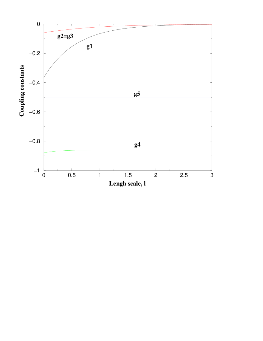
FIG. 3.: The renormalization group flow with initial conditions (90) and $y_{0}=0$. The couplings constants $g_{1},g_{2},g_{3}$ are renormalized to 0, whereas $g_{4}\to g_{4}^{*}$, and $g_{5}\to g_{5}^{*}$. The system therefore flows to a two component Luttinger liquid fixed point.

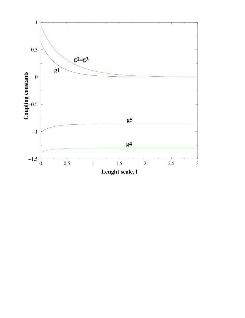
FIG. 4.: The renormalization group flow with initial conditions (90) and $y_{0}=1$. The couplings constants $g_{1},g_{2},g_{3}$ are renormalized to 0, whereas $g_{4}\to g_{4}^{*}$, and $g_{5}\to g_{5}^{*}$. The presence of a marginal perturbation preserving SU(3) symmetry does not suppress the two component Luttinger liquid behavior. However, by comparing with Fig. 3, it is seen that it changes the exponents at the fixed point.

FIG. 5.: Gap scalings for magnetization $m=1$. Lowest two energies $E_{0}(S_{z})$ and $E_{1}(S_{z})$ for each $S_{z}$ obtained by DMRG are plotted into $\Delta S^{tot,z}=0$ gap scaling: $10[E_{1}(S_{z})-E_{1}(S_{z})]$ vis $1/L)$, and $\Delta S^{tot,z}=1$ gap scaling: $E_{0}(S_{z}-1)+E_{0}(S_{z}+1)-2E_{0}(S_{z})$ vis $1/L$ with $S_{z}=L$. We have magnified the $\Delta S^{tot,z}=0$ gap by times to make the figure clear. The linear fittings are $E_{1}(S_{z})-E_{0}(S_{z})\sim 1/L$ and $E_{0}(S_{z}-1)+E_{0}(S_{z}+1)-2E_{0}(S_{z})\sim 1/L$ in thermodynamic limit. The chain lengths calculated by DMRG are $L=8$, $12$, $\ldots$, $40$.

REFERENCES

- [1] E. Dagotto and T. Rice, Science 271, 618 (1996).
- [2] F. D. M. Haldane, Phys. Rev. Lett. 50, 1153 (1983).
- [3] M. Azuma et al., Phys. Rev. Lett. 73, 3463 (1994).
- [4] G. Chaboussant et al., Phys. Rev. B 55, 3046 (1997).
- [5] H. Schulz, in Strongly Correlated Magnetic and Superconducting Systems, Vol. 478 of Lecture Notes in Physics, edited by G. Sierra and M. Martin-Delgado (Springer, Berlin, 1997).
- [6] E. Orignac, R. Citro, and N. Andrei, Low-energy behavior of the spin-tube model and coupled XXZ chains, 1999, article in preparation.
- [7] M. Oshikawa, M. Yamanaka, and I. Affleck, Phys. Rev. Lett. 78, 1984 (1997).
- [8] D. Cabra, A. Honecker, and P. Pujol, Phys. Rev. Lett. 79, 5126 (1997).
- [9] D. Cabra, A. Honecker, and P. Pujol, Phys. Rev. B 58, 6241 (1998), cond-mat/9802035.
- [10] R. Chitra and T. Giamarchi, Phys. Rev. B 55, 5816 (1997).
- [11] I. Affleck, in Fields, Strings and Critical Phenomena, edited by E. Brezin and J. Zinn-Justin (Elsevier Science Publishers, Amsterdam, 1988).
- [12] M. Reigrotzki, H. Tsunetsugu, and T. M. Rice, J. Phys. Condens. Matter 6, 9235 (1994).
- [13] S. R. White, Phys. Rev. Lett. 69, 2863 (1992).
- [14] S. R. White, Phys. Rev. B 48, 10345 (1993).
- [15] K. Kawano and M. Takahashi, J. Phys. Soc. Jpn. 66, 4001 (1997).
- [16] F. Mila, Eur. Phys. J. B 6, 201 (1998), cond-mat/9805029.
- [17] E. Lieb, T. D. Schultz, and D. Mattis, Ann. Phys. 16, 407 (1961).
- [18] K. Tandon et al., Phys. Rev. B 59, 396 (1999), cond-mat/9806111.
- [19] S. Pokrovskii and A. M. Tsvelik, Sov. Phys. JETP 66, 1275 (1987).
- [20] G. Fáth and P. B. Littlewood, Phys. Rev. B 58, R14709 (1998), cond-mat/9810259.
- [21] E. Gusev, Theor. Math. Phys. 53, 1018 (1983).
- [22] S. Gasiorowicz, Elementary Particle Physics (Wiley, New York, 1966), p. 261.
- [23] G. Uimin, JETP Lett. 12, 225 (1970).
- [24] B. Sutherland, Phys. Rev. B 12, 3795 (1975).
- [25] J. B. Parkinson, J. Phys. Condens. Matter 1, 6709 (1989).
- [26] H. Kiwata, J. Phys. Condens. Matter 7, 7991 (1995).
- [27] A. Schmitt, K. H. Mütter, and M. Karbach, J. Phys. A 29, 3951 (1996).
- [28] Z. Maassarani and P. Mathieu, Nucl. Phys. B 517, 395 (1998), cond-mat/9709163.
- [29] E. Lieb, T. D. Schultz, and D. Mattis, Ann. Phys. 16, 407 (1961).
- [30] I. Affleck and E. H. Lieb, Lett. Math. Phys. 12, 57 (1986).
- [31] I. Affleck, Nucl. Phys. B 265, 409 (1986).
- [32] I. Affleck, Nucl. Phys. B 305, 529 (1988).
- [33] E. Witten, Commun. Math. Phys. 92, 455 (1984).
- [34] A. Tsvelik, Quantum Field Theory in Condensed Matter Physics (Cambridge University Press, Cambridge, 1995).
- [35] I. Affleck, D. Gepner, T. Ziman, and H. J. Schulz, J. Phys. A 22, 511 (1989).
- [36] T. Ziman and H. J. Schulz, Phys. Rev. Lett. 59, 140 (1987).
- [37] H. J. Schulz, Phys. Rev. Lett. 64, 2831 (1990).
- [38] H. J. Schulz, in Proceedings of Les Houches Summer School LXI, edited by E. Akkermans, G. Montambaux, J. Pichard, and J. Zinn-Justin (North-Holland, Amsterdam, 1995), p. 533.
- [39] N. Kawakami and S. K. Yang, Phys. Rev. B 44, 7844 (1991).
- [40] C. A. Hayward et al., Phys. Rev. Lett. 75, 926 (1995).
- [41] F. Mila and X. Zotos, Europhys. Lett. 24, 133 (1993).
- [42] M. Ogata, M. U. Luchini, S. Sorella, and F. F. Assaad, Phys. Rev. Lett. 66, 2388 (1991).
- [43] R. Assaraf, P. Azaria, M. Caffarel, and P. Lecheminant, Metal-insulator transition in the one-dimensional SU(N) Hubbard model, 1999, cond-mat/9903057.
- [44] C. Itoi and M.-H. Kato, Phys. Rev. B 55, 8295 (1997).
- [45] C. Itoi and H. Mukaida, J. Phys. A 27, 4695 (1994).
- [46] It is interesting to note that a similar Hamiltonian enters in the theory of two dimensional melting (see eq. (3.16) in Ref. [50]).
- [47] J. M. Kosterlitz, J. Phys. C 7, 1046 (1974).
- [48] J. José, L. Kadanoff, S. Kirkpatrick, and D. Nelson, Phys. Rev. B 16, 1217 (1977).
- [49] T. Giamarchi and H. J. Schulz, Phys. Rev. B 39, 4620 (1989).
- [50] D. R. Nelson, Phys. Rev. B 18, 2318 (1978).
- [51] L. P. Kadanoff, Ann. Phys. 120, 39 (1979).
- [52] H. J. F. Knops and L. W. J. Den Ouden, Physica A 103, 597 (1980).
- [53] C. Itoi (unpublished).
- [54] F. D. M. Haldane, Phys. Rev. Lett. 45, 1358 (1980).
- [55] T. Giamarchi and H. J. Schulz, J. Phys. (Paris) 49, 819 (1988).
- [56] H. J. Schulz, in Correlated fermions and transport in mesoscopic systems, edited by T. Martin, G. Montambaux, and J. Tran Thanh Van (Editions frontières, Gif sur Yvette, France, 1996).
- [57] It is important to remark that the correlation functions have been calculated by using the fixed point Hamiltonian. This means that there are logarithmic corrections to the expressions that we quote due to asymptotic freedom. Such logarithmic corrections have been analyzed for instance in Refs. [35, 49] for SU(2) spin chains.
- [58] The conformal transformation was carried out right at the fixed point. For a system that does not sit exactly at the fixed point, there would be corrections coming from the irrelevant operators. This is the finite temperature counterpart of the logarithmic corrections that are obtained at .
- [59] O. Golinelli, T. Jolicoeur, and E. Sorensen, Incommensurability in the magnetic excitations of the bilinear-biquadratic spin-1 chain, 1998, cond-mat/9812296.
- [60] D. Sen, private communication.
- [61] S. Eggert and I. Affleck, Phys. Rev. B 46, 10866 (1992).
- [62] S. Qin, J. Lou, Z. Su, and L. Yu, in Density-Matrix Renomalization, Lecture Note in Physics, edited by I. Peschel, X. Wang, M. Kaulke, and K. Hallberg (Springer, Berlin, 1999).
- [63] S. Qin et al., Phys. Rev. B 56, 9766 (1997).
- [64] F. D. M. Haldane, Phys. Rev. Lett. 47, 1840 (1981).
- [65] J. L. Cardy, Scaling and Renormalization in Statistical Physics, Cambridge Lecture Notes in Physics (Cambridge University Press, Cambdridge, UK, 1996).