Phase transitions in finite systems = topological peculiarities
of the microcanonical entropy surface

Abstract

It is discussed how phase transitions of first order (with phase separation and surface tension), continuous transitions and (multi)-critical points can be defined and classified for finite systems from the topology of the energy surface $e^{S(E,N)}$ of the mechanical N-body phase space or more precisely of the curvature determinant $D(E,N)=\partial^{2}S/\partial E^{2}*\partial^{2}S/\partial N^{2}-(\partial^{2}S/\partial E\partial N)^{2}$ without taking the thermodynamic limit. The first calculation of the entire entropy surface $S(E,N)$ for a $q=3$-states Potts lattice gas on a $50*50$ square lattice is shown. There are two lines, where $S(E,N)$ has a maximum curvature $\sim 0$. One is the border between the regions in {$E,N$} with $D(E,N)>0$ and with $D(E,N)<0$, the other line is critical starting as a valley in $D(E,N)$ running from the continuous transition in the ordinary $q=3$-Potts model, converting at $P_{m}$ into a flat ridge/plateau (maximum) deep inside the convex intruder of $S(E,N)$ which characterizes the first order liquid–gas transition. The multi-critical point $P_{m}$ is their crossing.

Boltzmann’s gravestone has the famous epigraph:

$S=k*lnW$

which puts thermodynamics on the ground of mechanics [1, 2]. It relates the entropy $S$ to the volume $W(E,N,V)=\delta\epsilon*tr\delta(E-H_{N})$ of the energy ($E$) surface of the N-body phase space at given volume ($V$), the microcanonical partition sum. Here $\delta\epsilon$ is a suitable small energy constant, $H_{N}$ is the $N$-particle Hamiltonian, and

$$tr\delta(E-H_{N})=\int{\frac{d^{3N}p\;d^{3N}q}{(2\pi\hbar)^{3N}}\delta(E-H_{N})}.$$ (1)

The set of points on this surface defines the microcanonical ensemble (ME).

Today conventional thermodynamics is based on the canonical statistical mechanics as introduced by Gibbs[3]. In the thermodynamic limit ThL ($N\!\!\to\!\!\infty|_{N/V=const}$) the canonical ensemble (CE) is equivalent to the fundamental (ME) if the system is in a pure phase and the ThL exists.

The fundamental difference of microcanonical thermodynamics (MT) to conventional thermodynamics is that no non-mechanical quantities like temperature, heat, pressure have to be introduced a priori.

The link between ME and CE is established by Laplace transform. E.g. the usual grand canonical partition sum is the double Laplace transform of ME:

$$Z(T,\mu,V)=\int\rule{-9.95845pt}{0.0pt}\int_{0}^{\infty}{dE\;dN\;e^{-(E-\mu N)/T}tr\delta(E-H_{N})}.$$ (2)

This excludes all inhomogeneous situations, especially phase separations. There the entropy is non-extensive and the CE contains several Gibbs states at the same temperature. Consequently, the statistical fluctuations do not disappear in the CE even in the thermodynamic limit. This is the reason why Gibbs himself excluded phase separations in chapter VII of[3] in a footnote, page 75. At phase transitions the ME and the CE describe different physical situations. If one combines a small system of water at the specific energy $\epsilon_{1}$ of boiling water with a large heat bath at $100^{0}$C it will remain at $100^{0}$C but may convert into steam in $50\%$ of the cases. I.e. the fundamental assumption used e.g. by Einstein [1] that our “system changes only by infinitely little” does not hold.

It is important to notice that Boltzmann’s and also Einstein’s [1, 2] formulation allows for defining the entropy by $S_{micro}:=ln[W(E,N,V)]$ (in the following we use $S_{micro}$ for $S(E,N)$ if it is not clear) as a single valued, non-singular, in the classical case differentiable, function of all “extensive”, conserved dynamical variables. No thermodynamic limit must be invoked and the theory applies to non-extensive systems as well. Of course this is achieved by avoiding Gibbs-states, “equilibrium states” or “most random” states [4]. On the other hand fluctuations become then important and must be simulated by Monte Carlo methods. The microcanonical ensemble is the entire microcanonical N-body phase space without any exception. In MT the entropy is not “a measure of randomness” [4], it is simply the volume $e^{S(E,N,V)}$ of the energy surface. The latter point is extremely important as it allows to address even thermodynamically unstable systems like collapsing gravitating systems (for a recent application of MT to thermodynamical unstable, collapsing systems under high angular momentum see[5]). In so far it is the most fundamental formulation of equilibrium statistics[6, 7]. From here the whole thermostatics may be deduced. MT describes how $e^{S(E,N,V)}$ depends on the dynamically conserved energy, number of particles etc.. Of course we must assume that the system can be found in each phase-space cell of $e^{S}$ with the same probability.

Following Lee and Yang [8] phase transitions are indicated by singularities in $Z(T,\mu,V)$. Singularities of $Z(T,\mu,V)$, however, can occur in formula (2) in the thermodynamic limit only ($V\to\infty|_{N/V=\varrho,E/N=\varepsilon}$). For finite volume $Z(T,\mu,V)$ is a finite sum of exponentials and everywhere analytical. Only at points where $S(E,N)$ has a curvature $\geq 0$ will the integral eq.2 diverge in the thermodynamic limit. In these points, the Laplace integral 2 does not have a stable saddle point. Here van Hove’s concavity condition [9] for the entropy $S(E,N,V)$ of a stable phase is violated. Consequently we define phase transitions also for finite systems topologically by the points of non-negative curvature of the entropy surface $S(E,N,V)$ as a function of the mechanical, conserved “extensive” quantities like energy, mass, angular momentum etc..

Experimentally one identifies phase transitions of course not by the singularity of $Z(T,\mu)$ but by the interfaces separating coexisting phases, e.g. liquid and gas, i.e. by the inhomogeneities. The interfaces have three effects on the entropy:

1. There is an entropic gain by putting a part ($N_{1}$) of the system from the majority phase (e.g. liquid) into the minority phase (bubbles, e.g. gas), but this is connected with an energy-loss due to the higher specific energy of the “gas”-phase,

2. an entropic loss proportional to the interface area by the correlations between the particles in the interface, leading to the convex intruder in $S(E,N,V)$ and is the origin of surface tension [10],

3. and an additional mixing entropy for distributing the $N_{1}$-particles in various ways into bubbles.

At a (multi-) critical point two (or more) phases become indistinguishable and the interface entropy (surface tension) disappears.

Microcanonical thermostatics was introduced in great detail for atomic clusters and nuclei in [11]. In two further papers we showed how the surface tension can quantitatively be determined from the microcanonical $S(E,N,V)$ for realistic systems like small liquid metal drops [12, 13]. Needless to say that only by our extension of the definition of phase transitions to finite systems it make sense to ask the question: “How many particles are needed to establish a phase transition?” The results we are going to show here will again demonstrate that often $N$ does not need to be large in order to see realistic values (close to the known bulk values) for the characteristic parameters. Other examples where shown in our earlier papers[10, 12, 13].

In the following we investigate the 3-state Potts lattice-gas model on a 2-dim $L^{2}=50^{2}$ square lattice. We will see how the total microcanonical entropy surface $S(E,N)$ decovers even the most sophisticated thermostatic features as first order phase transitions, continuous phase transitions, critical and multicritical points even for finite systems and non-extensive systems. This demonstrates that the microcanonical statistics is in contrast to Schrödinger’s claim [14] quite able to handle not only gases but also phase transitions and critical phenomena. Important details like the separation of phases and the origin of surface tension can be treated. The singularity of the canonical partition sum at a transition of first order can be traced back to the loss of entropy due to the correlations between the surface atoms at phase boundaries [10].

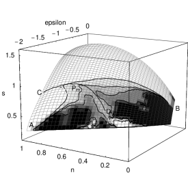
FIG. 1.: Entropy $s=\frac{1}{L^{2}}S_{micro}(\epsilon\!\!=\!\!E/L^{2},n\!\!=\!\!N/L^{2})$. The grey levels are as in fig.4: white regions: concave, pure phases (in $A$$P_{m}$$C$ ordered, “solid”, in $C$$P_{m}$$B$ disordered “gas”); black: convex, phase separation (“liquid–gas”); and light grey strips: critical branches; crossing: multicritical point $P_{m}$. If one plots $S_{micro}$ vs. $\beta$ and $\beta\mu$ like in CT the two wings $P_{m}A$ and $P_{m}B$ are mapped onto one-another in the figure 2 below. The black regions of the intruder get folded in between (see fig.3).

Briefly, a few words about our method which will be published in detail in [15]: The Hamiltonian is $H=-\frac{1}{2}\sum_{i,j}\delta_{\sigma i,\sigma j}$ ($i,j$ nearest neighbors). We covered all space $\{E=\epsilon*L^{2},N=n*L^{2}\}$ by a mesh with about $1000$ knots with distances of $\Delta\epsilon=0.04$ and $\Delta n=0.02$. Due to our limited computational resources (DEC-Alpha workstation) we could not use a significantly denser mesh. At each knot $\{\epsilon_{i},n_{k}\}$ we performed by microcanonical simulations ($\approx 2*10^{8}$ events) a histogram for the probabilities $P(\epsilon_{i},n_{k})$ for the system to be in the narrow region $(E_{i}\pm 4)*(N_{k}\pm 4)$ of phase space. Local derivatives $\beta=\left(\partial S(E,N)/\partial E\right)_{N}$, $\beta\mu=-\left(\partial S(E,N)/\partial N\right)_{E}$ in each histogram give the “intensive” quantities, so that the entire surfaces of $S(E,N)$, $\beta(E,N)$, $\beta\mu(E,N)$ can be interpolated. The first derivatives of the interpolated (smoothed) $\beta(E,N)$ and $\beta\mu(E,N)$ give the curvatures.

The figure 1 shows some of our recent results for $S(E/L^{2},N/L^{2})$ for the case of the diluted $q=3$ Potts model. Grid lines are in direction $[E-E_{0}(N)]/[E_{max}(N)-E_{0}(N)]=$const. resp. $N/L^{2}=$const.. The black region is the intruder at the first-order condensation transition (“liquid–gas coexistence”) with positive largest curvature of $S(E,N)$. This corresponds to the similar region in the Ising lattice gas, respectively the original Ising model as function of the magnetization. At the light grey strip $S(E,N)$ is critical with vanishing largest curvature. The line from point $C$ over the multicritical point $P_{m}$ to $D$ corresponds from $C$ to $P_{m}$ to the familiar continuous transition in the ordinary $q=3$ Potts model. At $P_{m}$ this line crosses the rim of the intruder from $A$ to $B$ which is the border of the first order transition. This crossing determines the multicritical point $P_{m}$ quite well at $\beta_{m}=1.48\pm 0.03$, $\beta\mu_{m}=-2.67\pm 0.02$ or $\epsilon_{m}\sim-1$, $n_{m}\sim 0.7$. From here the largest curvature starts to become $\,\raisebox{-2.15277pt}{$\stackrel{{\scriptstyle>}}{{\scriptstyle\sim}}$}\,0$. Naturally, $P_{m}$ spans a much broader region in {$\epsilon,n$} than in {$\beta,\beta\mu$}, remember here $S(E,N)$ is flat.

FIG. 2.: Contour plot of the entropy $s_{micro}(\beta,\beta\mu)$. One clearly sees the critical line where $s_{micro}(\beta,\beta\mu)$ becomes tripelvalued and/or at the ordinary Potts continuous transitions $\partial S/\partial\beta\sim-\infty$. Here several points of $S(E,N)$ from the entropy surface are folded onto one-another. That is the origin of the thick multi-valued (“critical”) line in $s_{micro}(\beta,\beta\mu)$.

If one plots the entropy $s_{micro}(\beta,\beta\mu)$ as function of the “intensive” variables $\beta\mu=-\partial S/\partial N$ and $\beta=\partial S/\partial E$, we obtain picture 2. This corresponds to the conventional grand-canonical representation if we would have calculated the grand canonical entropy from the Laplace transform $Z(T,\mu,V)$, eq.2. As there are several points $E_{i},N_{k}$ with identical $\beta,\beta\mu$, $s_{micro}(\beta,\beta\mu)$ is a multivalued function of $\beta,\beta\mu$. Here the entropy surface $S(E,N)$ is folded onto itself see fig.3 and in fig.2 these points show up as a black critical line (dense region). The backfolded branches of $S(E,N)$ are jumped over in eq. 2 and get consequently lost in $Z(T,\mu)$. This demonstrates the far more detailed insight one obtains into phase transitions and critical phenomena by microcanonical thermostatics which is not accessible by the canonical treatment.

In figure 4 the determinant of curvatures of $S(E,N)$:

$$D(E,N)=\left\|\begin{array}[]{cc}\frac{\partial^{2}S}{\partial E^{2}}&\frac{\partial^{2}S}{\partial N\partial E}\\ \frac{\partial^{2}S}{\partial E\partial N}&\frac{\partial^{2}S}{\partial N^{2}}\end{array}\right\|$$ (3)

is shown. On the diagonal we have the ground-state of the $2$-dim Potts lattice-gas with $\epsilon=-2n$, the upper-right end is the complete random configuration (not shown), with the maximum allowed excitation $\epsilon_{rand}=-\frac{2n^{2}}{q}$. In the upper right (white) $D>0$, both curvatures are negative. In this region the Laplace integral eq.2 has a stable saddle point. This region corresponds to pure phases.

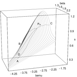
FIG. 3.: $s_{micro}(\beta,\beta\mu)$, the same as fig.2. The grey lines are for $\beta=$const. The backbending of the intruder left of $P_{m}$ which is hidden behind the thick critical line in fig.2 is clearly seen. This corresponds to the whole intruder of phase separation (black and grey in fig.4). The lines connect the points of $\partial s/\partial(\beta\mu)|_{\beta}=-\infty$ and thus correspond to the critical lines in fig.4. The positions of $A$,$B$,$D$,$C$ are only roughly indicated.

In the light gray region we have $D\sim 0$. This is the critical region. Here the largest eigenvalue of $D$ is $0$. Two branches cross here: One goes $\approx$ parallel to the ground state ($E\propto-2N$) from $A$ to $B$. This is a rim in $D(E,N)$, the border line between the region with $D(E,N)>0$, and the region with $D(E,N)<0$ (black) where we have the first order liquid—gas transition of the lattice-gas. The Laplace integral (2) has no stable saddle point and in the ThL the grand canonical partition sum (2) diverges. Here we have a separation into coexisting phases, e.g. liquid and gas. Due to the surface tension or the negative surface entropy of the phase boundaries, $S(E,N)$ has a convex intruder with positive largest curvature.

The other branch from $C$ to $P_{m}$ is a valley in $D(E,N)$. Here the largest curvature of $S(E,N)$ has a local minimum and $D\sim 0$ (it would be $D=0$ with a higher precision of the simulation), running from the point (near $C$) of the continuous phase transition at $n=1$ and $\epsilon=-1.57$ of the ordinary $q=3$-Potts model downwards to $P_{m}$. It converts below the crossing point $P_{m}$ into a flat ridge inside the convex intruder of the first order lattice-gas transition. The area of the crossing of the two critical branches $CP_{m}D$ and $AP_{m}B$ is the multi-critical region $P_{m}$ of the $q=3$ Potts lattice gas model.

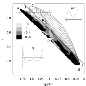
FIG. 4.: Contour plot of the determinant of curvatures $D(\epsilon\!\!=\!\!E/L^{2},n\!\!=\!\!N/L^{2})$. In the two light gray strips we have $D(\epsilon,n)\sim 0$. Here the transition is critical (continuous). The crossing point $P_{m}$ indicates the multicritical region. The two inlets show cuts along the line $f$$\leftrightarrow$$g$ ($\epsilon=-2n+0.28$) through the intruder with first order transition and negative $D$ (positive largest curvature). To understand the dramatic loss of information in the CT: The whole black and grey region (about half of the entire phase space !) gets lost, see also fig3. The other along $m$$\leftrightarrow$$n$ near to the ordinary q=3 Potts model ($n=0.88$) shows to the left the ordered phase with positive $D$, then the deep valley with nearly vanishing curvature and to the right the disordered (“gas”) phase.

Conclusion: Microcanonical thermostatics (MT) describes how the entropy $S(E,N)$ as defined entirely in mechanical terms by Boltzmann depends on the conserved “extensive” mechanical variables: energy $E$, particle number $N$, angular momentum $L$ etc. This allows to study phase transitions also in small and in non-extensive systems. If we define phase transitions in finite systems by the topological properties of the determinant of curvatures $D(E,N)$ (eq.3) of the microcanonical entropy-surface $S(E,N)$: a single stable phase by $D(E,N)>0$, a transition of first order with phase separation and surface tension by $D(E,N)<0$ , a continuous (“second order”) transition with $D(E,N)=0$, and a multi- critical point where more than two phases become indistinguishable by the branching of several lines with $D(E,N)=0$, then there are remarkable similarities with the corresponding properties of the bulk transitions.

The advantage of MT compared to CT is clearly demonstrated: About half of the whole phase space, the intruder of $S(E,N)$ or the non-white region in fig.4, gets lost in conventional canonical thermodynamics. Without any doubts this contains the most sophisticated physics of this system. Due to limited computer resources this could be demonstrated with only limited precision. We are convinced our conclusions will be verified by more extensive – and more expensive – calculations.
 
Acknowledgment: D.H.E.G thanks M.E.Fisher for the suggestion to study the Potts-3 model and to test how the multicritical point is described microcanonically. We are gratefull to the DFG for financial support.

REFERENCES

- [1] A. Einstein. Annalen der Physik, 9:417–433, 1902.
- [2] A. Einstein. Annalen der Physik, 14:354–362, 1904.
- [3] J.W. Gibbs. Elementary Principles in Statistical Physics, volume II of The Collected Works of J.Willard Gibbs. Yale University Press 1902,also Longmans, Green and Co, NY, 1928.
- [4] R.S. Ellis. Entropy, Large Deviations and Statistical Mechanics. Springer, New York, Heidelberg, 1985.
- [5] V. Laliena. http://xxx.lanl.gov/abs/cond-mat/9806241.
- [6] P. Ehrenfest and T. Ehrenfest. Begriffliche Grundlagen der statistischen Auffassung in der Mechanik, volume IV. Enzycl. d. Mathem. Wissenschaften, 1912.
- [7] P. Ehrenfest and T. Ehrenfest. The Conceptual Foundation of the Statistical Approach in Mechanics. Cornell University Press, Ithaca NY, 1959.
- [8] T. D. Lee and C. N. Yang. Phys. Rev., 87:410, 1952.
- [9] L. van Hove. Physica, 15:951, 1949.
- [10] D.H.E.Gross,A.Ecker,and X.Z.Zhang. Ann. Physik, 5:446 -452, http://xxx.lanl.gov/abs/cond-mat/9607150, 1996.
- [11] D.H.E. Gross. Physics Reports, 279:119–202, 1997.
- [12] D.H.E. Gross and M.E. Madjet. Microcanonical vs. canonical thermodynamics. http://xxx.lanl.gov/abs /cond-mat/9611192.
- [13] D.H.E. Gross and M.E. Madjet. Z.Physik B, 104:541–551, 1997 and http://xxx.lanl.gov/abs/cond–mat/9707100.
- [14] E. Schrödinger. Statistical Thermodynamics, a Course of Seminar Lectures, delivered in January-March 1944 at the School of Theoretical Physics. Cambridge University Press, London, 1946.
- [15] E. Votyakov and D.H.E. Gross. Total microcanonical entropy surface , continuous and first order phase transitions, critical lines and multicritical points for various finite q-state Potts lattice gases. HMI to be published, 1999.