ENERGY LANDSCAPES, SUPERGRAPHS, AND “FOLDING FUNNELS” IN SPIN SYSTEMS

I INTRODUCTION

The concept of energy landscapes has played a significant role in elucidating kinetics of protein folding [1, 2]. An energy landscape can be visualized by using the so called disconnectivity graphs [3] that show patterns of pathways between the local energy minima of a system. A pathway consists of consecutive moves that are allowed kinetically. The pathways indicated in a disconnectivity graph are selected to be those which provide a linkage at the lowest energy cost among all possible trajectories between two destinations. Thus, at each predetermined value of a threshold energy, the local energy minima are represented as divided into disconnected sets of minima which are mutually accessible through energy barriers. The local minima which share the lowest energy barrier are joined at a common node and are said to be a part of a basin corresponding to the threshold.

The disconnectivity graphs have proved to be useful tools to elucidate the energy landscape of a model of a short peptide [3] and of several simple molecular systems. In particular, Wales, Miller, and Walsh [4] have constructed disconnectivity graphs for the archetypal energy landscapes of a cluster of 38 Lennard-Jones atoms, the molecule of C₆₀, and 20 molecules of water. The work on the Lennard-Jones systems has been recently extended by Doye et al. [5]. The graph for a well folding protein is expected to have an appearance of a “palm tree.” This pattern has a well developed basin of the ground state and it also displays several branches to substantially higher lying local energy minima. Such a structure seems naturally associated with the existence of a folding funnel. The atomic level studies of the 4-monomer peptide considered by Becker and Karplus [3] yield a disconnectivity graph which suggests that this expected behavior may be correct. Bad folders are expected to have disconnectivity graphs similar to either a “weeping willow” or a “banyan tree” [3, 4] in which there are many competing low lying energy minima.

We accomplish several tasks in this paper. The first of these, as addressed in Sec. II, is to construct disconnectivity graphs for two lattice heteropolymers the dynamics of which have been already studied exactly [6]. One of them is a model of a protein, in the sense that it has excellent folding properties, and we shall refer to it as a good folder. The other has very poor folding properties, i.e. it is a bad folder and is thus a model of a random sequence of aminoacids. We show that, indeed, only the good folder has a protein-like disconnectivity graph.

In Sec. III we study the archetypal energy landscapes corresponding to small two dimensional (2D) Ising spin systems with the ferromagnetic and spin glassy exchange couplings. We demonstrate that disordered ferromagnets have protein-like disconnectivity graphs whereas spin glasses behave like bad folders. This is consistent with the concept of minimal structural frustration [7], or maximal compatibility, that has been introduced to explain why natural proteins have properties which differ from those characterizing random sequences of aminoacids. It is thus expected that spin systems which have the minimal frustration in the exchange energy, i.e. the disordered ferromagnets, would be the analogs of proteins. In fact, we demonstrate that the kinetics of “folding,” i.e. the kinetics of getting to the fully aligned ground state of the ferromagnet by evolving from a random state, depends on temperature, $T$, the way a protein does. Finding a ground state of a similarly sized spin glass takes place significantly longer.

The disconnectivity graphs characterize the phase space of a system and, therefore, they relate primarily to the equilibrium properties – the dynamics is involved only through a definition of what kinds of moves are allowed, but their probabilities of being implemented are of no consequence. Note that even if the disconnectivity graph indicates a funnel-like structure, the system may not get there if the temperature is not right. Thus a demonstration of the existence of a funnel must involve an actual dynamics. In fact, another kind of connectivity graphs between local energy minima has been introduced recently precisely to describe the $T$-dependent dynamical linkages [8] in the context of proteins. We shall use the phrase a “dynamical connectivity graph” to distinguish this concept from that of a “disconnectivity graph” of Becker and Karplus. The idea behind the dynamical connectivity graphs is rooted in a coarse grained description of the dynamics through mapping of the system’s trajectories to underlying effective states. In ref. [8], the effective states are the local energy minima arising as a result of the steepest descent mapping. In ref. [9], the steepest descent procedure is followed by an additional mapping to a closest maximally compact conformation. The steepest descent mapping has been already used to describe glasses [10] and spin glasses [11] in terms of their inherent, or hidden, valley structures.

In the dynamical connectivity graphs, the linkages are not uniform in strength. Their strengths are defined by the frequency with which the two effective states are visited sequentially during the temporal evolution. The strengths are thus equal to the transition rates and they vary significantly from linkage to linkage and as a function of $T$. An additional characteristic used in such graphs is the fraction of time spent in a given effective state, without making a transition. This can be represented by varying sizes of symbols associated with the state.

In the context of these developments, it seems natural to combine the two kinds of coarse-graining graphs, equilibrium and dynamical, into single entities – the supergraphs. Such supergraphs can be constructed by placing the information about the $T$-dependent dynamical linkages on the energy landscape represented by the disconnectivity graph. This procedure is illustrated in Sec. IV for the case of the two heteropolymers discussed in Sec. II. The procedure is then applied to selected spin systems. In each case, knots of significant dynamical connectivities within the ground state basin develop around a temperature at which the specific heat has a maximum. These knots disintegrate on lowering the $T$ if the system is a spin glass or a bad folder. For good folders and non-uniform ferromagnets the dynamical linkages within the ground state basin remain robust.

We hope that this kind of combined characterization, by the supergraphs, of both the dynamics and equilibrium pathways existing in many body systems might prove revealing also in the case of other systems, e.g., such as the molecular systems considered in ref. [4].

II ENERGY LANDSCAPES IN 2D LATTICE PROTEINS

Lattice models of heteropolymers allow for an exact determination of the native state, i.e. of the ground state of the system, and are endowed with a simplified dynamics. These two features have allowed for significant advancement in understanding of protein folding [12].

Here, we consider two 12-monomer sequences of model heteropolymers, $A$ and $B$, on a two-dimensional square lattice. These sequences have been defined in terms of Gaussian contact energies (the mean equal to $-1$ and the dispersion to 1, roughly) in ref. [6]. They have been studied [6, 8] in great details by the master equation and Monte Carlo approaches. Sequences $A$ and $B$ have been established to be the good and bad folders respectively. Among the $15\;037$ different conformations that a 12-monomer sequence can take, 495 are the local energy minima for sequence $A$ and 496 for sequence $B$. The minima are either $V$- or $U$-shaped. The $U$-shaped minima are those in which a move that does not change the energy is allowed, provided there are no moves that lower the energy. Both kinds of minima arise as a result of the steepest descent mapping from states generated along a Monte Carlo trajectory and both kinds are included in the disconnectivity graphs.

Constructing a disconnectivity graph requires determination of the energy barriers between each pair of the local energy minima. We do this through an exact enumeration. We divide the energy scale into discrete partitions of resolution $\Delta E$ (we consider $\Delta E$=0.5) and ask between what minima there is a pathway which does not exceed the threshold energy set at the top of the partition. These minima can then be grouped into clusters which are disconnected from each other. Local minima belonging to one cluster are connected by pathways in which the corresponding barriers do not exceed a threshold value of energy whereas the local minima that belong to different clusters are separated by energy barriers which are higher than the threshold level. At a sufficiently high value of the energy threshold all minima belong to one cluster. Enumeration of the pathways involves storing a table of size $15\;037\times 14$ because each conformation may have up to 14 possible moves within the dynamics considered in ref. [6]. (16-monomer heteropolymers can also be studied in this exact way – within any resolution $\Delta E$.)

Figure 1 shows the resulting disconnectivity graphs for sequence $A$. For clarity, we show only this portion of the graph which involves the local minima with energies which are smaller than $-5$ (there are 206 such minima). Throughout this paper, the symbol $E$ denotes energy measured in terms of the coupling constants in the Hamiltonian and is thus a dimensionless quantity. The native state, denoted as NAT in the Figure 1, belongs to the most dominant valley. One can see that the graph contains a remarkable “palm tree” branch that provides a linkage to the native state. This branch is a place within which a dynamically defined folding funnel is expected to be confined to. The large size of this branch associated with a big energy gap between the native state and other minima indicates large thermodynamic stability. At low temperatures, the glassy effects set in and contributions due to non-native valleys become significant. The local minimum denoted by TRAP in Figure 1 has been identified in ref. [6] as giving rise to the longest lasting relaxation processes in the limit of $T$ tending to 0.

The disconnectivity tree for sequence $B$ is shown in Figure 2. Again, only the minima with energies smaller than $-5$ are displayed (there are 203 such minima). In this case, there are several local energy minima which are bound to compete with the native state. The corresponding branches have comparable lengths and morphologies. The dynamics is thus expected not to be confined merely to the native basin. Instead, the system is bound to be frustrated in terms of what branch to choose to evolve in. At low $T$’s the valley containing the TRAP conformation is responsible for the longest relaxation and poor folding properties.

Other examples of disconnectivity trees for protein related systems have been recently constructed with the use of Go-like models [13, 14] (in which the aminoacid-aminoacid interactions are restricted to the native contacts) and they confirm the general pattern of differences in morphology between good and bad foldability as illustrated by Figures 1 and 2.

It should be noted that there are many ways to map out the multidimensional energy landscape of proteins. In particular, extensive energy landscape explorations for the HP lattice heteropolymers have been done with the use of the pathway maps [15, 16, 17]. The pathway maps show the actual microscopic paths through conformations. The paths are enumerated either exactly or statistically, and thus provide a detailed but implicit representation of the energy landscape. The resulting “flow diagrams” indicate patterns of allowed kinetic connections between actual conformations, together with the energy barriers involved. They can also be additionally characterized by Monte Carlo determined probabilities to find a given path at a temperature under study. In this way, preferable pathways and important transition states can be identified. This approach is similar in spirit to the one undertaken by Leopold et al. [18] in which the folding funnel is identified through determination of weights associated with paths that lead to the native state.

The coarse grained representation of energy landscapes in protein-like systems through the disconnectivity trees is quite distinct from that obtained through the pathway maps. The disconnectivity graphs indicate only the one best path for each pair of the local energy minima by showing the terminal points and the value of the energy barrier necessary to travel this path. This reduced information is precisely what allows one to provide an explicit and essentially automatic visualization of the energy landscapes.

FIG. 1.: The disconnectivity graph for the 12-monomer sequence $A$. The dotted area is shown again in Figure 10 together with the dynamical connectivities. $N_{c}$ is a symbolic notation for a label of an energy minimum, based on computer generated listing.

FIG. 2.: Similar to Figure 1 but for sequence $B$. The dotted area is shown expanded in Figure 11.

The $T$-dependent frequencies of passages between conformations in the pathway maps give an account of the dynamics in the system. This information on the dynamics, however, does not easily fit the description provided by the disconnectivity graphs. The steepest descent mapping to the local energy minima that we propose here is, on the other hand, a perfect match.

III ENERGY LANDSCAPES IN 2D SPIN SYSTEMS

We now consider the spin systems. The Hamiltonian is given by $H\;=\;\sum_{<ij>}J_{ij}S_{i}S_{j}$ where $S_{i}$ is $\pm 1$, and the exchange couplings, $J_{ij}$, connect nearest neighbors on the square lattice. The periodic boundary conditions are adopted. When studying spin systems, a frequent question to ask about the dynamics is what are the relaxation times – characteristic times needed to establish equilibrium. Here, however, we are interested in quantities which are analogous to those asked in studies of protein folding. Specifically, what is the first passage time $t_{0}$? The first passage time is defined as the time needed to come across the ground state during a Monte Carlo evolution that starts from a random spin configuration. A mean value of $t_{0}$ in a set of trajectories (here, we consider 1000 trajectories for each $T$) will be denoted by $\left<t_{0}\right>$ and the median value by $t_{g}$. $t_{g}$ is an analogue of the folding time, $t_{f}$ of ref. [6]. At low temperatures, the physics of relaxation and the physics of folding essentially agree [6]. At high temperatures, however, the relaxation is fast but finding a ground state is slow due to a large entropy. Both for heteropolymers and spin systems the $T$-dependence of the characteristic first passage time is expected to be $U$-shaped. The fastest search for the ground state takes place at a temperature $T_{min}$ at which the $T$-dependence has its minimum.

The $U$-shape dependence of $t_{f}$ originates in the idea of a low $T$ glassy phase in heteropolymers advocated by Bryngelson and Wolynes [7] within the context of the random energy model. It was subsequently confirmed in numerical simulations of lattice models [15, 19, 17]. This shape is, actually expected for most disordered systems, including those involving spins. However, experimentalists measuring spin systems typically would not ask about the first passage time (at high $T$).

This overall behavior is illustrated in Figure 3 for two $5\times 5$ spin systems. The Gaussian couplings of zero mean and unit dispersion are selected for the spin glassy (SG) 2$D$ system. The disordered ferromagnetic system (DFM) is endowed with the exchange couplings which are the absolute values of the couplings considered for SG. Figure 3 shows that $t_{g}$ does depend on $T$ in the $U$-shaped fashion. $T_{min}$ for SG and DFM are comparable in values but the “folding” times for DFM are more than 4 times shorter than for SG. The times are defined in terms of the number of Monte Carlo steps per spin.

FIG. 3.: The main figure shows the $T$-dependence of $t_{g}$ – the median time to find the ground state – for $5\times 5$ DFM and SG systems. The top inset compares $t_{g}$ to $t_{0}$ on the logarithmic time scale. The divergence of the two times at low $T$’s indicates a substantial spreading out of the distribution of $t_{0}$. This distribution, $P(t_{0})$, is shown in the lower inset for temperatures corresponding to $T_{min}$.

FIG. 4.: Distribution of energy barriers (highest elevation points) across trajectories. The solid line is for the $4\times 4$ DFM system. It shows barriers for all trajectories which connect local minimum $\alpha$ to another local minimum $\beta$. The lowest of them, $E_{\alpha\beta}$, is used as threshold in the disconnectivity graph. The dotted line is for a $5\times 5$ DFM and for trajectories which go from a local energy minimum $\phi$ to the ground state. The energy barrier $E_{\phi 0}$ is obtained through the approximate enumeration as described in the text. The other values are obtained by generating 50000 random connecting trajectories.

Figure 3 establishes some of the analogies between the heteropolymers and the spin systems. We now consider the disconnectivity graphs for selected $L\times L$ spin systems with $L$=4 and 5. For both system sizes, the list of the local energy minima is obtained through an exact enumeration. Determination of an energy barrier between two minima requires adopting some approximations. Suppose that the two minima differ by $n$ spins. There are then $n!$ possible trajectories which connect the two minima, assuming that a) no spin is flipped more than once, b) no other spins (or “external” spins) are involved in a pathway. These trajectories can be enumerated for $L$=4 but not for $L$=5. In the latter case we adopt the following additional approximation. We first identify the $n(n-1)(n-2)(n-3)$ list of the first four possible steps in any trajectory together with the highest energy elevation reached during these four steps. We choose $m$=1500 trajectories which accomplish the smallest elevation. We then consider the next two-step continuations of the selected trajectories and among the $m(n-4)(n-5)$ continuations again select $m$ which result in the lowest elevation, and so on until all $n$ spins are inverted. The lowest elevation among the final set of the $m$ trajectories is an estimate of the energy threshold used in the disconnectivity diagram. This approximate method, when applied to the $L$=4 systems, generates results which agree with the exact enumeration. Figure 4 shows that our method clearly beats determination of barriers based on totally random trajectories (but still restricted to overturning of the $n$ differing spins).

Flipping of the “external” spins was found to give rise to an occasional reduction in the barrier height. We could not, however, come up with a systematic inclusion of such phenomena in the calculations and the resulting disconnectivity graphs have barriers which are meant to be estimates from above. The topology of the graph is expected to depend little on details of such approximations.

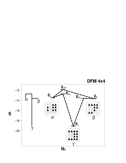
FIG. 5.: Examples of pathways between three local energy minima, $\alpha,\beta$, and $\gamma$, in a $4\times 4$ DFM. The corresponding spin configurations are shown by arrows. The resulting disconnectivity graph is shown on the left.

In some cases, the barrier for a direct travel from one minimum to another was found to be higher than when making a similar passage via an intermediate local energy minimum. An example of this situation is shown in Figure 5. However, this lack of transitivity, resulting from the approximate nature of the calculations, does not affect the disconnectivity graph because the states $\gamma$ and $\beta$ of Figure 5 are mutually accessible at energy $E_{\beta\gamma}$. Then, at a higher energy $E_{\alpha\gamma}$, state $\alpha$ is thus also accessible. If, at this energy level, the system can transfer between the states $\alpha$ and $\gamma$ then it can also transfer to state $\beta$.

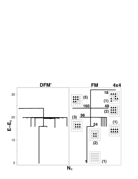
FIG. 6.: The disconnectivity graphs for the FM and DFM’ $4\times 4$ systems, as defined in the text. The arrows in the boxes show examples of the corresponding spin configurations. The numbers indicate the degree of degeneracy and the numbers in brackets indicate numbers of distinct geometries for the inverted domains to take at the energy considered. For a uniform antiferromagnetic system the disconnectivity graph looks qualitatively similar to the one characterizing FM but the ground state is the only $V$-shaped local energy minimum of the system.

We now present specific examples of disconnectivity graphs for several distinct spin systems.

Figure 6 shows the case of a $4\times 4$ uniform ferromagnet (FM). The energy landscape of the FM is not analogous to that of a protein because uniform exchange couplings generate states with high degrees of degeneracies. These degeneracies can be split either by a randomization. Figure 6 also shows a graph for a $L=4$ DFM’ system in which the $J_{ij}$’s are random numbers from the [0.9,1.1] interval – this is the case of a small perturbation away from the uniform FM. The graph for DFM’ has an overall appearance like the one for FM except for the lack of a high energy linkage to a set of state which cease to be minima. Another difference is the disappearance of all remaining $U$-shaped minima and formation of new true minima at somewhat spread out energies. In the uniform $L=4$ ferromagnet, there are five $V$-shaped energy minima: one is the ground state and the other four higher energy states are degenerate. In addition, there are 346 states which are the $U$-shaped energy minima. An example of what happens in a $U$-shaped minimum is shown in Figure 7. Here, the system can move between the 3- and 4-spin domains without a change in the energy. The 4-spin domain forms a $U$-shaped minimum but the 3-spin state is not a minimum because there is a move to a lower energy state. Only the 4-spin domain states would be shown in the disconnectivity graph.

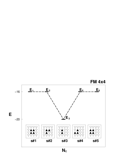
FIG. 7.: Examples of spin configurations in the $4\times 4$ FM system.

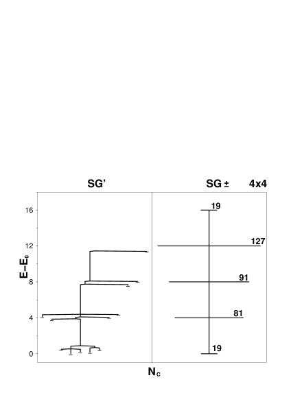
FIG. 8.: The disconnectivity graphs for the $4\times 4$ spin glassy systems: with the Gaussian (SG’) and with the $\pm 1$ couplings (SG $\pm$). The numbers correspond to the number of $U$-shaped minima at an energy shown in the graph.

Figure 8 shows the disconnectivity graphs for two $L=4$ spin glassy systems. The right hand panel shows the case of $J_{ij}=\pm 1$. The left hand panel shows a spin glass (SG’) with the exchange couplings which are randomly positive or negative and with their magnitudes coming from the interval [0.9,1.1] – this is the random sign counterpart of the DFM’ system. In both spin glassy systems of Figure 8 the allocation of signs to the couplings is identical. In the $\pm 1$ case, all minima, including the degenerate ground state, are $U$-shaped. The SG’ system, on the other hand, has a graph with an overall structure akin to that corresponding to the $\pm 1$ system with one important difference: the ground state is not degenerate and thus the ground state basin splits into several competing valleys.

The differences between the good and bad spin “folders” amplify as the system size is increased. As an illustration, Figure 9 shows the disconnectivity graphs for the $5\times 5$ DFM and SG – with the Gaussian couplings. The DFM systems has a very stable and well developed valley corresponding to the ground state whereas the SG system has many competing valleys. Thus indeed, DFM is a spin analogue of a protein whereas SG is an analogue of a random sequence of aminoacids.

FIG. 9.: The disconnectivity graphs for the $5\times 5$ DFM and SG systems (the top panels) and the corresponding representation of the energy landscapes (the bottom panels).

The disconnectivity graphs can be represented in a form that gives a better illusion of an actual landscape, as shown in the bottom panels of Figure 9. The lines shown there connect the local energy minima to their energy barriers and then to the next minimum, and so on, forming an envelope of the original graph. This form is less cluttered and will be used in Sec. V. This envelope representation shows merely the smallest scale variations in energy and omits passages with large barriers.

IV DYNAMICAL CONNECTIVITY GRAPHS FOR LATTICE HETEROPOLYMERS

We now construct the supergraphs for the lattice heteropolymers discussed in Sec. II. The strengths of the dynamical linkages have been already determined in ref. [8] at several temperatures. Here, however, we plot the linkages on the graphs that represent the energy landscapes, i.e. we rearrange the labels associated with the local energy minima. We discuss only the case of $T=T_{min}$ which is equal to 1.0 for both sequences $A$ and $B$.

FIG. 10.: Dynamical connectivity graph for sequence $A$ at $T$=1.0 plotted against the background of the disconnectivity graph. The dynamical linkages are restricted to the dotted region of Figure 1 and only this portion of the disconnectivity graph is shown.

FIG. 11.: Similar to Figure 10 but for sequence $B$.

Figures 10 and 11 shows the supergraphs for sequences $A$ and $B$ respectively. The sizes of the circles are proportional to an occupancy of the minimum during the folding time. Similarly, the thicknesses of the lines connecting the circles are proportional to the connectivity (the linking frequency) between them. For clarity, we do not show connectivities which account for less than $1\%$ of all combined dynamical connectivities. The disconnectivity graphs themselves are drawn in dotted lines. All relevant dynamics is confined to these portion of the of the disconnectivity graphs which were marked, in Figures 1 and 2, by the dotted lines and are now magnified in Figures 10 and 11.

An inspection of the supergraphs clearly shows differences between the two sequences. Sequence $A$ has many inter-valley linkages but the linkages to the native basin, and the occupancies of conformations within that basin, are substantial. These are manifestations of a fast folding dynamics. For sequence $B$, on the other hand, the linkages tend to wither uncooperatively in multiple valleys. In addition, the combined occupancies away from the native valley outweigh the dynamical effects within the valley. On lowering the temperature, linkages in various valleys become disconnected and tend to avoid the native valley more and more, as discussed in ref. [8].

V DYNAMICAL CONNECTIVITY GRAPHS FOR SPIN SYSTEMS

We now generate dynamical linkages for two spin systems, $L=5$ DFM and SG of Sec. III, and place them on the plots of the energy landscape. The “envelope” form of the representation of the landscape is chosen here, mostly for esthetic reasons. The connectivities are determined based on 200 Monte Carlo trajectories of a fixed length of 5000 steps per spin. The duration of these trajectories exceeds the “folding time” many times, at the temperatures studied, and thus the connectivities displayed refer to the essentially equilibrium situations (the equilibrium dynamics for heteropolymers $A$ and $B$ is illustrated in ref. [8]). The connectivity rates were updated any time (in terms of single spin events and not in terms of steps per spin) there is a transition from a local energy minimum to a local energy minimum, after the steepest descent mapping. Again, the $1\%$ display cutoff has been implemented when making the figure.

The main parts of Figures 12 and 13 show the supergraphs obtained at a temperature which corresponds to the $T$-location of the peak in specific heat. These temperatures, 1.8 for DFM and 1.4 for SG, are also close to $T_{min}$. The insets show the dynamically relevant parts of the energy landscape at lower temperatures. For the DFM, the dynamics becomes increasingly confined to the ground state basin when the temperature is reduced. On the other hand, for the SG, the dynamics in the ground state basin becomes less and less relevant, with a higher local energy minimum absorbing the majority of moves. This is indeed what happens with bad folding heteropolymers.

If we restrict counting of the transition rates only to the “folding stage,” i.e. till the ground state is encountered, the qualitative look of the supergraph for $T$ close to $T_{min}$ is as in the equilibrium case. The states involved are mostly the same but there is, by definition, only one link to the ground state per trajectory.

The dynamical connectivity graphs in 3D $10\times 10\times 10$ DFM systems are qualitatively similar to the 2D graphs but the underlying disconnectivity graphs are harder to display due to a substantially larger number of the energy minima.

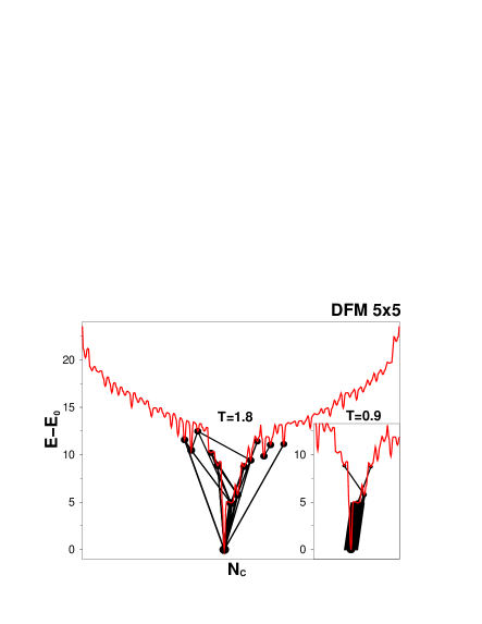
FIG. 12.: The dynamical-equilibrium supergraph for the $5\times 5$ DFM system at $T$=1.8. The inset shows the portion that is relevant at $T$=0.9.

FIG. 13.: The supergraph for the $5\times 5$ SG system at $T$=1.4. The insets show the portions which are relevant at two lower temperatures. The ground state configuration is shown at the top.

In this paper we have pointed out the existence of many analogies between protein folding and dynamics of spin systems. These analogies have restrictions. For instance the simple Ising spin systems in 3$D$ have continuous phase transitions, in the thermodynamic limit, and not the first-order-like that are expected to characterize large proteins [20]. This difference, however, is not crucial in the case of small systems. More accurate spin analogs of proteins, with the first order transition, can be constructed but the object of this paper was to discuss the basic types of spin systems.

On the other hand, it should be pointed out that these analogies are also more extensive. Consider, for instance, the Thirumalai [21] criterion for good foldability of proteins. The criterion considers two quantities: the specific heat and the structural susceptibility of a heteropolymer. The latter is a measure of fluctuations in the structural deviations away from the native state. Both quantities have peaks at certain temperatures. The criterion specifies that if the two temperatures coincide a heteropolymer is a good folder. This is quite similar to what happens in uniform and disordered 3D ferromagnets: the peaks (singularities) in magnetic susceptibility and specific heat are located at the same critical temperature. On the other hand, in spin glasses, the broad maximum in the specific heat is located at a temperature which is substantially above the freezing temperature associated with the cusp in the susceptibility. Also in this sense then, spin glasses behave like bad folders.

The coarse-graining supergraphs that analyse dynamics in the context of the system’s energy landscape may become a valuable tool to understand complex behavior of many body systems.

REFERENCES

- [1] J. D. Bryngelson, J. N. Onuchic, N. D. Socci, and P. G. Wolynes, Proteins: Struct., Funct., Genet. 21, 167 (1995).
- [2] P. G. Wolynes, Proc. Natl. Acad. Sci. USA 93, 14249 (1996).
- [3] O. M. Becker and M. Karplus, J. Chem. Phys. 106, 1495 (1997).
- [4] D. J. Wales, M. A. Miller and T. R. Walsh, Nature 394, 758 (1998).
- [5] J. P. K. Doye, M. A. Miller, and D. J. Wales, preprint cond-mat 9903305
- [6] M. Cieplak, M. Henkel, J. Karbowski, and J. R. Banavar, Phys. Rev. Lett. 80, 3654 (1998); M. Cieplak, M. Henkel, and J. R. Banavar, Cond. Matt. Phys. (Ukraine) 2, 369 (1999).
- [7] J. D. Bryngelson and P. G. Wolynes, J. Phys. Chem. 93, 6902 (1989); J. D. Bryngelson and P. G. Wolynes, Proc. Natl. Acad. Sci. USA 84, 7524 (1987).
- [8] M. Cieplak and T. X. Hoang, Phys. Rev. E 58, 3589 (1998).
- [9] M. Cieplak, S. Vishveshwara, and J. R. Banavar, Phys. Rev. Lett. 77, 3681 (1996); M. Cieplak and J. R. Banavar, Fold. Des. 2, 235 (1997).
- [10] F. H. Stillinger and T. A. Weber, Phys. Rev. A 28, 2408 (1983); Science 225, 983 (1984).
- [11] M. Cieplak and J. Jaeckle, Z. Phys. B 66, 325 (1987).
- [12] K. A. Dill, S. Bromberg, S. Yue, K. Fiebig, K. M. Yee, D. P. Thomas, and H. S. Chan, Protein Science 4, 561 (1995).
- [13] M. S. Li and M. Cieplak, preprint, cond-mat 9904421 (unpublished).
- [14] M. A. Miller and D. J. Wales, preprint, cond-mat 9904304 (unpublished).
- [15] R. Miller, C. A. Danko, M. J. Fasolka, A. C. Balazs, H. S. Chan, and K. A. Dill, J. Chem. Phys. 96, 768 (1992).
- [16] H. S. Chan and K.A. Dill, J. Chem. Phys. 99, 2116 (1993); H. S. Chan and K. A. Dill, J. Chem. Phys 100, 9239 (1994).
- [17] H. S. Chan and K. A. Dill, Proteins: Struct., Funct., Genet. 30, 2 (1998).
- [18] P. E. Leopold, M. Montal, and J. N. Onuchic, Proc. Natl. Acad. Sci. USA, 89, 8721 (1992).
- [19] N. D. Socci and J. N. Onuchic, J. Chem. Phys. 101, 1519 (1994).
- [20] See e.g. A. Gutin, V. Abkevich, and E. Shakhnovich, Phys. Rev. Lett. 80, 208 (1998); A. Sali, E. Shakhnovich, and M. Karplus, Nature (London), 369, 248 (1994).
- [21] C. J. Camacho and D. Thirumalai, Proc. Natl. Acad. Sci. USA 90, 6369 (1993); D. K. Klimov and D. Thirumalai, Phys. Rev. Lett. 76, 4070 (1996).