Spin structure of impurity band of semiconductors in two and three-dimensional cases

Abstract

The exchange interaction between electrons located at different randomly distributed impurities is studied for small density of impurities. The singlet-triplet splitting $2J(R)$ is calculated for two Coulomb centers at a distance $R$. Interpolated formulas are found which work for all distances $R$ from zero to infinity. The data from atomic physics are used for the interpolation in three-dimensional case. For two-dimensional case the original calculations are performed to find asymptotic behavior of the splitting at large $R$, the splitting for the “two-dimensional helium atom” ($R=0$) and the splitting at $R=a_{B}$, where $a_{B}$ is the effective Bohr radius. The spin structure of impurity band is described by the Heisenberg Hamiltonian. The ground state of a system consists of localized singlets. The new results are obtained for the distribution of the singlet pairs in the ground state. These results are exact at low density. The problem is reduced to a non-trivial geometric problem which is solved in the mean field approximation and by computer modeling. The density of free electrons is found as a function of temperature and the distribution function of the singlet-triplet transitions energies is calculated. Both functions are given in an analytical form.

I Introduction

The structure of the impurity band of semiconductors has been widely studied during the last two decades both theoretically and experimentally (See monograph[2] ). In the early theoretical studies the spin structure of the impurity band was completely ignored. Recent experiments suggest that the spin structure is very important for the variable range hopping conductivity, especially near the metal-non-metal transition[3, 4, 5, 6, 7, 8].

The exchange interaction must be the main mechanism of the spin-spin interaction in the impurity band. It appears as a result of the overlap of the wave functions of different states. The scale of this interaction decreases exponentially with increasing distance between the states. Thus, this interaction becomes the most important one near the metal-non-metal transition. In this region the scale of the interaction is of the order of the binding energy of a single impurity.

In this paper we study the spin structure of the impurity band created by Coulomb impurities in both two and three dimensional cases in the limit of low density of impurities. In the two-dimensional case the impurities may be located either outside or inside the plane of electron gas. We assume that all impurities are occupied by one electron. In this case we can consider the coordinates of the occupied centers as random variables without any correlations.

Our study of the spin structure is based upon the Heisenberg Hamiltonian which takes into account the spin-spin interaction of the electrons localized at different randomly distributed impurities.

$$H=\sum_{i\neq k}J_{ik}(I/2+{\bf s_{i}\cdot s_{k}}),$$ (1)

where ${\bf s}$ is spin 1/2 operator, $I$ is a unit matrix, and $i,k$ denote different impurity atoms. The sum is over all pairs of impurities. The density of impurities is assumed to be small.

This problem has a long story[9, 10, 11, 12, 13, 14, 15, 16]. The following important results have been obtained:
1. The ground state of the system consists of local singlets.
2. Rosso[9], Thomas and Rosso[14], Andres et al.[12] used different selfoconsistent approaches to get the distribution of the excitation energies of the singlet-triplet transitions.
3. Bhatt and Lee[13, 11] worked out a computational scaling approach which is exact at small density of impurities. They have also mentioned a drastic difference between the Heisenberg and Ising models.
4. As far as we know all previous authors used simplified versions for the function $J(R)$.

Our paper pursues the following goals:
1. We analyze the existing methods to find the distribution of excitation energies and propose a new modification for one-, two- and three-dimensional cases. Our approach is exact at low densities and it allows to get an approximate analytical expression for this distribution.
2. To get an estimate for the energy of spin ordering one needs a reliable calculation of the coefficients $J_{ik}$ which are defined here as $1/2$ of the singlet-triplet splitting for the two states corresponding to the impurities $i$ and $k$. We have performed these calculations for a pair of the Coulomb centers at a distance $R_{ik}$. The result of the computations is a function $J(R)$ which is reliable at all distances from zero to infinity.

The paper is organized as follows. In Section 2 we consider Hamiltonian Eq.(1) in the case of small impurity density. We show that the ground state mostly consists of independent singlets. We show that the problem of finding these singlets can be reduced to a non-trivial geometric problem. We solve it in a mean field approximation and by computer modeling. The solution of this problem gives the distribution function $F(E)$ for the energies of the singlet-triplet transitions for a given function $J(R)$.

In Section 3 we calculate $J(R)$ and its inverse function $R(J)$. For the $3D$-case we present interpolated formulae which are based upon the results of well-known calculations for two hydrogen atoms. These calculations include analytical results for large distances[19], numerical calculations at intermediate distances, and known results for the singlet-triplet splitting of the He atom. Similar interpolated formulae are presented for the $2D$-case. They are based upon our original calculations given in the appendices. We present an analytical expression for $J(R)$ at large distances, a numerical result for $J(a_{B})$, and variational calculations for a “two-dimensional He atom”.

In the Conclusion we discuss the distribution function of singlet-triplet splittings $F(\ln\varepsilon)$, where $\varepsilon=J/J(0)$, and the density of free spins $\rho(T)$ at finite temperature $T$. These two functions are the final results of our paper.

II Ground state and excited states of the Heisenberg Hamiltonian in the impurity band

A The structure of the ground state

We find the ground state and excited states of the Hamiltonian Eq.(1) using the following properties of $J_{ik}$.

• All $J_{ik}>0$, which means an antiferromagnetic interaction.

• The density of impurities $n$ is assumed to be small, so that the average distance between them is larger than the characteristic length of the exponential decay of $J_{ik}$. This means there is a very large dispersion of $J_{ik}$. In fact we shall assume that if $J_{ik}>J_{lm}$, then $J_{ik}\gg J_{lm}$. Thus, we ignore the cases when the distance $R_{ik}$ is very close to the distance $R_{lm}$, assuming that these two pairs are not very far from each other.

To understand the physics of the problem it is very helpful to consider the Hamiltonian (1) with four impurities only (Fig. 1a). From a general principle one can conclude[17] that the energy spectrum consists of six levels, one level with spin $S=2$, three levels with $S=1$, and two levels with $S=0$. Let us assume that $J_{12}$ is much larger than all other $J_{ik}$ in this problem. Then the ground state wave function describes two singlets at sites (1,2) and (3,4). It is easy to write the energy of the ground state and the first excited state assuming

$$J^{\prime}=\sum^{\prime}J_{ik}\ll J_{12},$$ (2)

where the sum includes all $J_{ik}$ except $J_{12}$ and $J_{34}$. The ground state energy $E_{0}$ and the energy of the first excited state $E_{1}$ are given by the equations

$$E_{0}=-J_{12}-J_{34}+J^{\prime}/2;\quad E_{1}=-J_{12}+J_{34}+J^{\prime}/2.$$ (3)

The physical meaning of Eq. (3) is simple. Two singlets (1,2) and (3,4) do not interact with each other if condition (2) is fulfilled. The $J^{\prime}/2$ terms come from the first term in the Hamiltonian (1).

In this approximation the excitation energy is $E=2J_{34}$. The ground state has a total spin $S=0$ while the first excited state has $S=1$.

Bhatt and Lee[13, 11] take into account the next approximation for the excitation energy

$$E=2J_{34}+(J_{13}-J_{23})(J_{24}-J_{14})/J_{12}.$$ (4)

Since $J_{12}$ is the largest term, the second term should be small. It looks like it can change the ground state from singlet to triplet if $J_{34}$ is unusually small. However, such configurations are extremely rare. It happens because in the case of small $J_{34}$ one should consider Fig.1b with 6 spins rather than Fig.1a. Indeed, very small $J_{34}$ means a long distance between impurities 3 and 4. It is more likely that in this situation some other strong singlet (5,6) is the nearest neighbor of the impurity 4 rather than the singlet (1,2).

In this 6-spin system we have 2 strongly connected groups of spins, namely 1,2,3 and 4,5,6. Assume that $J_{12}$ and $J_{56}$ provide the strongest bonds in each group. Suppose there is no interaction between the groups. Then, the ground state in each of them is a degenerate doublet. Altogether the system is 4-fold degenerate. If one takes into account $J_{34}$ the degeneracy of the ground state will be lifted. One gets a singlet and a triplet with the energy splitting $2J_{34}$. On the other hand, the general 6-spin problem can be solved assuming that both $J_{12}$ and $J_{56}$ are infinite. In this approximation one gets the same result: the ground state is a singlet and the excitation energy $E=2J_{34}$. It follows that the other bonds connecting the two groups, like $J_{35}$ may contribute to the excitation energy only in the second order of perturbation theory. This contribution will contain a small dimensionless coefficient like $J_{35}/J_{12}$ and it may be neglected. Thus, it is not necessary to take into account the renormalization of the weak bonds due to their strong neighbors in the limit of small density. Bhatt and Lee also mention[11] that their computations show the triplet ground state in very rare cases.

Thus, we assume that the ground state energy of any even number of impurities has $S=0$ and the system can be split into localized singlets. To find the pairs of impurities which form the singlet in the ground state we propose the following geometric problem.
1. For every impurity in the system find its nearest neighbor.
2. Take the pair with the smallest distance. Generally, the nearest neighbor of a site A does not have site A as its nearest neighbor. But for the closest pair this is the case.
3. This closest pair forms a singlet with the largest binding energy. To find all other singlets remove both sites of the first pair. Go to point 1 and continue until all the singlets will be found.
The same geometric problem has been proposed by Thomas and Rosso[14] for three-dimensional case.

Assuming that all neighboring $J_{ik}$ are very different one can write the total energy of the lowest state in the form

$$E_{0}=-\sum_{s}J_{ik}+{1\over 2}\sum_{other}J_{ik},$$ (5)

where the first sum includes all pairs which form singlets and the second one includes all other pairs.

One can prove that the distribution of singlets, obtained as a solution of the problem above, gives the minimum of total energy. Suppose, for example, that the solution prescribes the configuration of singlets (1,2), (3,4) and (5,6), for impurities with the numbers from 1 to 6. One can show that any other location of singlets at the same impurities, like (1,3), (2,5) and (4,6), has larger energy.

We mention first that the contribution to the energy from all other impurities like 7,8… is the same at all configurations of singlets of six chosen impurities. Suppose now that $J_{12}\gg J_{34},J_{56}$. Then all other $J_{ik}$ connecting the six impurities are also less than $J_{12}$. Indeed, if one of them were larger, it would be used to form a singlet instead of $J_{12}$. Thus, any rearrangement of the pairs within 6 impurities that destroys singlet (1,2) increases the total energy. In the same way one can show that rearrangement of singlets in the system of four impurities 3,4,5,6 also increases the total energy. The same consideration can be done for any even number of impurities. Thus, the solution of the above geometric problem gives the ground state of the system.

B Solution of geometric problem and distribution function of excitation energies

We start with the simplest mean field approximation. Suppose we are at the stage where all pairs with distance less than $R$ are removed and we want to find the residual impurity density $n(R)$. The crucial point of the mean field approximation is that we neglect correlations in the positions of the remaining impurities except that they cannot be closer to one another than $R$.

We start with the two-dimensional case. Let us draw a circle around each impurity with the radius $R$. There will be no other impurities inside the circles. Now increase the radii from $R$ to $R+dR$ and calculate how many impurities occur in the rings between $R$ and $R+dR$. The total number of these impurities gives the decrease of $N(R)$, where $N(R)=Sn(R)$ and $S$ is the total area of the system. Thus, one gets the equation

$$dN(R)=-N(R)2\pi R\tilde{n}(R)dR.$$ (6)

Here $\tilde{n}(R)$ is the density of the impurities outside the circles. It is slightly larger than $n(R)$ (see below), but in the simplest mean field approximation we ignore this difference.

It is convenient to introduce the dimensionless coordinate $X=\sqrt{\pi n_{0}}R$ and the normalized number of particles (or density) $\rho(X)=n/n_{0}\equiv N/N_{0}$. Here $n_{0}=n(0)$ is the initial concentration of particles. The differential equation for $\rho(X)$ at $\tilde{n}=n$ has the form

$$d\rho=-2X\rho^{2}dX.$$ (7)

The solution of this equation with the condition $\rho(0)=1$ is

$$\rho_{2}(X)={1\over{1+X^{2}}},$$ (8)

where $\rho_{2}(X)$ is the two-dimensional density. Similar calculations for the three- and one-dimensional cases give

$$\rho_{d}(X)={1\over{1+X^{d}}}.$$ (9)

Here $X=(4\pi/3n_{0})^{1/3}R$ at $d=3$ and $X=2n_{0}R$ at $d=1$. This distribution has been obtained by Rosso[9] for $d=3$. One can show that at small $X$ the above results are exact, including $X^{d}$-corrections. Bhatt[10] has pointed out that it is not exact at large $X$. We believe that the exact distribution has a following form at large $X$

$$\rho_{d}(X)={1\over b_{d}X^{d}},$$ (10)

where the coefficient $b_{d}\neq 1$ and it depends on the dimensionality of space $d$. It follows from Eq.(10) that the average density $n(R)$ is independent of $n_{0}$ at large values of $R$ and it is of the order of $R^{-d}$. This is because the average distance between impurities cannot be smaller than $R$ by definition, and there are no reasons for it to be substantially larger than $R$. That is why we believe that Eq.(10) is exact at large $X$. Our computer modeling confirms this point and it gives us the values $b_{d}$.

We propose an improved mean field approach which takes into account the fact that the density $\tilde{n}$ outside the circles is slightly larger than the average density $n(R)$, because there are no impurities inside the circles. For example, at $d=2$, one gets

$$\tilde{n}=\frac{N}{S-N\pi R^{2}\alpha},$$ (11)

where $N\pi R^{2}\alpha$ is the excluded area inside $N$ circles. We have introduced a free parameter $\alpha<1$, which takes into account the overlap of the circles. Its value can be extracted from comparison with numerical computations.

Eq. (11) can be generalized for any $d$ to get a differential equation in $\rho_{d}$

$$\frac{d\rho_{d}}{dX^{d}}=-\frac{\rho_{d}^{2}}{1-\alpha_{d}\rho_{d}X^{d}}.$$ (12)

The solution is given by the following transcendental equation:

$$X^{d}=\frac{1-\rho_{d}^{b_{d}}}{b_{d}\rho_{d}}$$ (13)

with $b_{d}=\alpha_{d}+1$. It is worth mentioning that if we would neglect the “circles” overlapping ($b_{d}\equiv 2$), then the solution of Eq. (13) is

$$\rho_{d}(X)=\frac{1}{X^{d}+\sqrt{1+X^{2d}}},$$ (14)

which is an underestimate for large distances. In the general case, for $1<b_{d}<2$, the analytical solution of the transcendental equation (13) can be obtained only for large and small values of $X$.

$$\rho_{d}\approx\left\{\begin{array}[]{ll}1-X^{d}+\frac{3-b_{d}}{2}X^{2d}+\cdots,&X\ll 1\\ \frac{1}{b_{d}X^{d}}\left(1-\left(\frac{1}{b_{d}X^{d}}\right)^{b_{d}}+\cdots\right),&X\gg 1\end{array}\right.$$ (15)

We performed computer simulations of this problem for the one-, two- and three-dimensional cases. The results are shown in Fig. 2 (a) together with the simple mean field approximation of Eq. (9). We found that fitting our numerical data using Eq. (13) shows excellent agreement if we choose $b_{1}=1.67,\ b_{2}=1.49,\ b_{3}=1.15$. It would be natural to think that the simple mean field approach with $\alpha=0$ becomes exact for large values of $d$.

Unfortunately, Eq. (13) does not have an analytical solution for all $X$ and so it is not convenient for our purpose. We found that the simple interpolated formula

$$\rho_{d}(X)=\frac{1}{X^{d}+\sqrt{1+(b_{d}-1)^{2}X^{2d}}},$$ (16)

which resembles Eq.(14), describes the residual density well for the whole range of distances. The comparison of this formula with the results of computer modeling is shown in Fig. 2 (b),(c),(d) for d= 1,2,3. Below we use only Eq. (16) with the values of $b_{d}$ obtained above.

III Calculation of $J(R)$

A Three-dimensional case

The spin-spin interaction constant is the splitting energy between the ground states for total spin $S=1$ and $S=0$

$$2J=E_{g}^{S=1}-E_{g}^{S=0}\equiv^{3}\Sigma_{u}^{+}-^{1}\Sigma_{g}^{+}$$

for hydrogen-like molecule, where nuclei are represented by two impurities. Hereafter we use effective atomic units (a.u.) which means that all distances are measured in units of the effective Bohr radius $a_{B}=\hbar^{2}\epsilon/m^{*}e^{2}$, and energies in units of $m^{*}e^{4}/\hbar^{2}\epsilon^{2}$, where $m^{*}$ is the effective carrier mass, and $\epsilon$ is the dielectric constant.

We propose a simple interpolated formula for the exchange constant based on the most accurate numerical calculations of the hydrogen molecule [18] and the following asymptotic expression[19] for large $R$:

$$2J(R)\approx 1.636R^{5/2}\exp(-2R).$$ (17)

We found $J(0)$ from the data for the singlet-triplet splitting of the helium atom[22].

$$2J(0)=0.770\ \mbox{a.u.}$$

The numerical data[18] show that the behavior of the logarithm of the exchange constant for small $R$ is well described by a second order polynomial.

To obtain the interpolated formula we match the second derivative of $\ln\left(J(R)\right)$. In two regions it has the following behavior

$$\frac{\partial^{2}\ln(J)}{\partial R^{2}}\approx\left\{\begin{array}[]{ll}-2\tilde{A},&R\leq 1\\ -\frac{5}{2R^{2}},&R\gg 1,\end{array}\right.$$ (18)

where $\tilde{A}$ is the matching constant. The simplest formula that satisfies both conditions is

$$\frac{\partial^{2}\ln(J)}{\partial R^{2}}=-\frac{2\tilde{A}}{1+4/5\tilde{A}R^{2}}$$ (19)

After integrating twice we obtain

$$\ln(J) = \ln(J(0))-\gamma R-\frac{5}{2}AR\arctan(AR)+\frac{5}{4}\ln(1+A^{2}R^{2}),$$ (20)

where $A$ and $\gamma$ are connected by equation

$$A=\sqrt{4\tilde{A}/5}=\frac{4(2-\gamma)}{5\pi}.$$ (21)

This interpolated formula has one fitting parameter $\gamma$ and the correct asymptotic behavior.

The parameter $\gamma$ has to be chosen to match small distances in an optimal way. The least square method gives $\gamma=0.1$. The final equation is

$$2J_{3}(R)=0.770\left(1+0.23R^{2}\right)^{5/4}\exp\left(-0.1R-1.210R\arctan\left(0.484R\right)\right)\\$$ (22)

For further calculations we need the inverse function $R(J)$ as well. Because of the exponential character of the exchange constant, the inverse function depends on energy logarithmically. Therefore, we performed interpolation for the function $R(x)$, where $x=\ln(J(0)/J)$. The result is

$$R_{3}=\frac{x}{2}+\frac{3.5x}{1+\frac{3.5x}{1.69+0.68\ln(1+x)}}$$ (23)

The interpolated curves and all available data are shown in Fig. 3a.

B Two-dimensional case with in-plane impurities.

We are unaware of any calculations of $J(R)$ for the two-dimensional case. We have considered a general problem when the motion of the electrons is confined to a plane, but the Coulomb impurities are at distances $h_{1}$ and $h_{2}$ outside the plane. However, in this paper only the calculations for in-plane impurities ($h_{1}=h_{2}=0$) are presented. The results for the general case will be published elsewhere[23].

The case of the in-plane impurities corresponds to a $2D$ hydrogen-like molecule with the Hamiltonian

$$\hat{H}=-\frac{\Delta_{1}}{2}-\frac{\Delta_{2}}{2}-\sum_{j,i=1}^{2}\frac{1}{\sqrt{(x_{i}\pm a)^{2}+y_{i}^{2}}}+\frac{1}{\sqrt{(x_{1}-x_{2})^{2}+(y_{1}-y_{2})^{2}}}+\frac{1}{R}$$ (24)

When $R\gg 1$ the singlet-triplet splitting constant is calculated by making use the semiclassical approach [19, 20, 21] (see Appendix A). We obtained the following result:

$$2J(R)=30.413\,R^{7/4}\exp(-4R)$$ (25)

To provide the point $R=0$ we performed variational calculations for the two-dimensional helium atom. We found that (See Appendix B)

$$E(^{1}S) = -11.635\ \mbox{a.u.}$$ (26)

$$E(^{3}S) = -8.193\ \mbox{a.u.}$$ (27)

$$2J(0) = 3.567\,(\pm 1\%)\ \mbox{a.u.}$$ (28)

Finally, we performed numerical calculations based on the method described in [21] for the point $R=1$. Using the same method as in the $3D$-case we get the following interpolated formulas for $J(R)$ and $R\left(\ln(J_{0}/J)\right)$:

$$2J_{2}(R) = 3.567\left(1+1.81R^{2}\right)^{7/8}\exp\left(-0.3R-2.355R\arctan\left(1.346R\right)\right)$$ (29)

$$R_{2} = \frac{x}{4}+\frac{3x}{1+\frac{3x}{0.50+0.28\ln(1+x)}},$$ (30)

$$x = \ln\left(J(0)/J)\right).$$ (31)

These results are shown in Fig. 3b.

IV Conclusion

We obtained an analytical expression (16) for the dimensionless density of impurities which form singlet pairs with a distance larger than $R$. We have also calculated the strength of the spin-spin interaction $J$ and obtained analytical expressions for the function $R(J)$ for the three-dimensional (23) and the two-dimensional (30) cases. Combining Eq. (16) with Eqs. (23) or (30) one can calculate an analytical expression for the density of singlet pairs $n(E)/2$ that has a singlet-triplet energy splitting smaller than $E=2J$. At finite temperature $T$ the pairs with $E<T$ are destroyed by a thermal motion. Therefore, at a given temperature the function $n(E)$ at $E=T$ gives the density of free spins in the system which contribute to the Curie susceptibility. Thus, we obtain an analytical expression for the density of free spins $n(T)$.

We have also calculated the distribution function of excitation energy in a logarithmic scale. It is defined as follows

$$F(\ln(\varepsilon))=\frac{1}{2}\frac{d\,n}{d\,\ln(\varepsilon)}\equiv\frac{n_{0}}{2}\frac{d\,\rho}{d\,R}\frac{d\,R}{d\,\ln(\varepsilon)},$$ (32)

where $\varepsilon=E/(2J(0))\equiv J/J(0)$.

The analytical expression for $F(\ln(\varepsilon))$ based on Eqs. (16), (23), (30) is quite cumbersome. In the two limits of large and small energies (or small and large distances) the behavior of $F$ in the leading order is

$$\frac{F_{2D}}{n_{0}}\approx\left\{\begin{array}[]{ll}10.56\pi n_{0}a_{B}^{2}\ln(1/\varepsilon),&\qquad\varepsilon\longrightarrow 1\\ \frac{16}{1.49\pi n_{0}a_{B}^{2}}\left[\ln(1/\varepsilon)\right]^{-3},&\qquad\varepsilon\longrightarrow 0;\end{array}\right.$$ (33)

$$\frac{F_{3D}}{n_{0}}\approx\left\{\begin{array}[]{ll}128\pi n_{0}a_{B}^{3}\left[\ln(1/\varepsilon)\right]^{2},&\qquad\varepsilon\longrightarrow 1\\ \frac{9}{1.15\pi n_{0}a_{B}^{3}}\left[\ln(1/\varepsilon)\right]^{-4},&\qquad\varepsilon\longrightarrow 0.\end{array}\right.$$ (34)

Our results for $\rho(T)=n(T)/n_{0}$ are shown by the full lines in Fig. 4 (a), (b) for the two-dimensional and the three-dimensional cases. We choose two different dimensionless densities $n_{0}$ for each case. They are $\pi n_{0}a_{B}^{2}=0.1$ and 0.025 for $2D$ and $4\pi n_{0}a_{B}^{3}/3=0.004$ and 0.016 for $3D$.

The dependence of the dimensionless distribution function $F/n_{0}$ for the two-dimensional and the three-dimensional cases for the same two donor densities $n_{0}$ are presented on Fig. 4 (c), (d) by the full lines.

The most important features of both functions are the long logarithmic tails in the regions of low temperature and low energy. Similar behavior has been obtained by Bhatt and Lee[11]. Note that $\rho(T)$ decreases with increasing density $n_{0}$. This is not the case for the distribution function. Larger density corresponds to larger distribution function $F$ at large energies. This is because the derivative $n_{0}^{-1}dn/dR$ is larger for larger density $n_{0}$ at small $R$. However, the dimensionless distribution function $F(\ln\varepsilon)$ is normalized to 1/2. That is why the functions for different densities cross each other at some energy. Thus, at small energies the larger distribution function corresponds to smaller density.

To clarify the role of the functions $J(R)$, which have been found here, we have calculated the density of free spins $\rho(T)$ and the distribution function $F(\ln(\varepsilon))$ for a simplified function $J_{s}(R)$ used in Ref.[11].

$$J_{s}(R) = J(0)\exp(-2R/a_{B})\qquad\mbox{for 3D,}$$ (35)

$$J_{s}(R) = J(0)\exp(-4R/a_{B})\qquad\mbox{for 2D.}$$ (36)

In these calculations we used our residual density $\rho(R)$. The results are shown in Fig. 4 by the dashed lines. One can see that the difference is large. The distribution function for our more accurate form of the exchange constant became narrower and the decline in the beginning is steeper. This comes from the different behaviors at small distances.

It is interesting to compare the numerical scaling calculations by Bhatt and Lee[11] with our method of calculation $n(R)$. We have found that at the smallest density used in Ref. [11] both methods give similar results, but for larger densities there is a small deviation. We think that both methods are exact in the limit of small densities, but the method of Bhatt and Lee works in a wider range, because they take into account the renormalization of weak bonds caused by their strong neighbors. However, the great advantage of our method is that it gives an analytical expression for $n(E)$.

A Exchange constant for $2D$ Hydrogen-like molecule

The exchange constant for the Hamiltonian (24) is determined by

$$2J = (E_{g}^{S=1}-E_{g}^{S=0})\ \equiv(E_{A}-E_{S}),\quad\mbox{ where }$$ (A1)

$$\hat{H}\Psi_{S} = E_{S}\Psi_{S},$$ (A2)

$$\hat{H}\Psi_{A} = E_{A}\Psi_{A}.$$ (A3)

Because of the Fermi statistics the two-electron wave function is antisymmetric with respect to permutation. Therefore, the symmetric coordinate wave function corresponds to spin $S=0$ and the antisymmetric one corresponds to $S=1$.

Let us consider the more general Hamiltonian

$$\hat{H}=-\frac{\Delta_{1}}{2}-\frac{\Delta_{2}}{2}+V_{a}({\bf r}_{1}+{\bf a})+V_{a}({\bf r}_{2}+{\bf a})+V_{b}({\bf r}_{1}-{\bf a})+V_{b}({\bf r}_{2}-{\bf a})+\frac{1}{|{\bf r}_{1}-{\bf r}_{2}|}+\frac{1}{R},$$ (A4)

where $V_{a}$ and $V_{b}$ are effective potentials of interaction between the electron and the corresponding atomic residue, which is of the Coulomb type far from the atoms: $V_{a,b}\rightarrow-1/r,\ r-\rightarrow\infty$. The electron energy

$$E=-\alpha^{2}/2-\beta^{2}/2-1/R,$$

is accurate up to terms $\sim 1/R^{2}$. Here $\alpha^{2}/2$ and $\beta^{2}/2$ are electron binding energies in the given “atom”.

When $R\gg 1$ the most appropriate method for determination of the energy terms splitting due to the spin-spin interaction is the Gor’kov-Pitaevskii method [19, 20, 21].

Since $J(R)$ is exponentially small as $R\rightarrow\infty$, $\Psi_{A}$ and $\Psi_{S}$ are solutions of the same Schrödinger equation, and therefore, with exponential accuracy their combinations

$$\Psi_{1,2}=\frac{\Psi_{S}\pm\Psi_{a}}{\sqrt{2}}$$

are also the solutions of the same Schrödinger equation with the Hamiltonian (A4). They correspond to the states of “distinguishable” particles, when, e.g. for $\Psi_{1}({\bf r_{1},r_{2}})$, the first electron is principally located near the first ion at $x=-a$ and the second electron near the second ion with $x=a$. Here $R\equiv 2a$ is the distance between “nuclei”, which we place at the points $\pm a$ on the $x$ axis. In the main region of the electron distribution, the wave functions $\Psi_{1,2}$ are products of the atomic single-particle wave functions with the asymptotic behavior of the radial atomic wave functions of the electron in the Coulomb field of the atomic residue being determined by the formulas

$$\varphi_{a}(r)=A_{\alpha}r^{1/\alpha-1/2}e^{-\alpha r},\qquad\varphi_{b}(r)=A_{\beta}r^{1/\beta-1/2}e^{-\beta r}.$$ (A5)

Indeed, for large $r$ the potential is $U\sim-1/r$, and the single-particle wave function of the electron obeys the equation

$$-\frac{\Delta}{2}\varphi-\frac{1}{r}\varphi=-\frac{\alpha^{2}}{2}\varphi.$$

It has the asymptotic solution (A5) up to $\varphi/r^{2}$ accuracy. The coefficients $A_{\alpha,\beta}$ are determined by the behavior of the wave functions of the electron inside the atoms.

It is possible to show[21] that

$$2J=-2\int\left[\Psi_{2}\frac{\partial\Psi_{1}}{\partial x_{1}}-\Psi_{1}\frac{\partial\Psi_{2}}{\partial x_{1}}\right]_{x_{1}=x_{2}}~{}dx_{2}~{}dy_{1}~{}dy_{2}.$$ (A6)

Our main purpose is to find the wave function $\Psi_{1,2}$.

Let us suppose that $\Psi_{1,2}$ has the form

$$\Psi_{1}(\vec{r}_{1},\vec{r}_{2}) = \phi_{\alpha}(|\vec{r}_{1}+\vec{a}|)\phi_{\beta}(|\vec{r}_{2}-\vec{a}|)\chi(\vec{r}_{1},\vec{r}_{2}),$$ (A7)

$$\Psi_{2}(\vec{r}_{1},\vec{r}_{2}) = \phi_{\alpha}(|\vec{r}_{2}+\vec{a}|)\phi_{\beta}(|\vec{r}_{1}-\vec{a}|)\chi(\vec{r}_{2},\vec{r}_{1}),$$ (A8)

where $\phi_{\alpha,\beta}$ have the behavior of (A5) and $\chi$ is a slowly varying function of $r_{1}$ and $r_{2}$. Substituting $\Psi_{1}$ into the wave equation and neglecting the second derivatives of $\chi$, we obtain

$$\alpha\frac{\partial\chi}{\partial x_{1}}-\beta\frac{\partial\chi}{\partial x_{2}}+\left[\frac{1}{\sqrt{(x_{1}-x_{2})^{2}+(y_{1}-y_{2})^{2}}}+\frac{1}{2a}-\frac{1}{a-x_{1}}-\frac{1}{a+x_{2}}\right]\chi=0.$$ (A9)

Equation (A9) is valid under the conditions

$$|x_{1,2}|\leq a,y_{12}\equiv|y_{1}-y_{2}|\ll\sqrt{a}$$ (A10)

$$R\alpha,R\beta\gg 1,R|\alpha-\beta|\ll 1.$$ (A11)

The general solution of (A9) is

$$F(C_{1}(x_{1},x_{2}),C_{2}(\chi,x_{1},x_{2},y_{12})=0,$$ (A12)

where $C_{1},\ C_{2}$ are integrals of the motion of the ordinary differential equations:

$$\frac{dx_{1}}{\alpha}=-\frac{dx_{2}}{\beta}=-\frac{d\chi}{\chi}\left[\frac{1}{\sqrt{(x_{1}-x_{2})^{2}+y_{12}^{2}}}+\frac{1}{2a}-\frac{1}{a-x_{1}}-\frac{1}{a+x_{2}}\right]^{-1}.$$

Hence

$$\chi(x_{1},x_{2},y_{12})=\frac{\exp\left(-\frac{x_{1}}{2a\alpha}\right)\left[\sqrt{(x_{1}-x_{2})^{2}+y_{12}^{2}}-x_{1}+x_{2}\right]^{\frac{1}{\alpha+\beta}}}{[a-x_{1}]^{1/\alpha}[a+x_{2}]^{1/\beta}}f\left(\frac{x_{1}}{\alpha}+\frac{x_{2}}{\beta}\right),$$ (A13)

where the unknown function $f(u)$ is determined from the fact that $\chi\longrightarrow 1$ when $x_{1}\longrightarrow-a,\ x_{2}$ is arbitrary, or when $x_{2}\longrightarrow a$ and $x_{1}$ is arbitrary. Finally, after expanding $|\vec{r}\pm a|\simeq|a\pm x|+y_{12}^{2}/2|a\pm x|$ in the exponent, we obtain

$$\Psi_{1}(\vec{r}_{1},\vec{r}_{2}) = A_{\alpha}A_{\beta}\left(a+x_{1}\right)^{\frac{2-\alpha}{2\alpha}}\left(a-x_{2}\right)^{\frac{2-\beta}{2\beta}}\times$$ (A15)

$$\times\exp\left[-a(\alpha+\beta)+\beta x_{2}-\alpha x_{1}-\frac{\alpha y_{1}^{2}}{2(a+x_{1})}-\frac{\beta y_{2}^{2}}{2(a-x_{2})}\right]\chi(\vec{r}_{1},\vec{r}_{2}),$$

$$\chi(x_{1},x_{2},y_{12}) =$$ (A16)

$$\left\{\begin{array}[]{l}e^{-\frac{a+x_{1}}{2a\alpha}}\left[\frac{2a}{a-x_{1}}\right]^{\frac{1}{\alpha}}\alpha^{-\frac{\alpha}{(\alpha+\beta)\beta}}\left[\frac{\beta(a+x_{1})+\alpha(a+x_{2})}{a+x_{2}}\right]^{\frac{1}{\beta}}\left[\frac{\sqrt{(x_{1}-x_{2})^{2}+y_{12}^{2}}-x_{1}+x_{2}}{\sqrt{\left(\beta(a+x_{1})+\alpha(a+x_{2})\right)^{2}+(\alpha y_{12})^{2}}+\beta(a+x_{1})+\alpha(a+x_{2})}\right]^{\frac{1}{\alpha+\beta}}\\ e^{-\frac{a-x_{2}}{2a\beta}}\left[\frac{2a}{a+x_{2}}\right]^{\frac{1}{\beta}}\beta^{-\frac{\beta}{(\alpha+\beta)\alpha}}\left[\frac{\beta(a-x_{1})+\alpha(a-x_{2})}{a-x_{1}}\right]^{\frac{1}{\alpha}}\left[\frac{\sqrt{(x_{1}-x_{2})^{2}+y_{12}^{2}}-x_{1}+x_{2}}{\sqrt{\left(\beta(a-x_{1})+\alpha(a-x_{2})\right)^{2}+(\beta y_{12})^{2}}+\beta(a-x_{1})+\alpha(a-x_{2})}\right]^{\frac{1}{\alpha+\beta}}\end{array}\right.$$ (A17)

Here the upper expression is given for $x_{1}+x_{2}\leq 0$, and the lower expression for $x_{1}+x_{2}\geq 0$.

Substituting (A15) in Eq. (A6), and differentiating only the exponential we obtain

$$2J=+2(\alpha+\beta)\int_{-a}^{a}\left[\Psi_{1}\Psi_{2}\right]_{x_{1}=x_{2}=x}\,d\,x\,d\,y_{1}d\,y_{2}$$ (A18)

Introducing the notations $\mu=\alpha+\beta$ and $\nu=\beta-\alpha$ and taking into consideration the fact that at the approximation (A10)

$$\sqrt{\left[(\beta+\alpha)(a-x)\right]^{2}+(\beta y_{12})^{2}}+(\beta+\alpha)(a-x)\approx 2(\beta+\alpha)(a-x).$$

the formula (A18) transforms to

$$2J(\alpha,\beta,R)=R^{\frac{2}{\alpha}+\frac{2}{\beta}-\frac{1}{\mu}}e^{-\mu R}\left[D\left(\alpha,\beta,R\right)+D\left(\beta,\alpha,R\right)\right],$$ (A19)

where $D\left(\alpha,\beta,R\right)$ is the following function:

$$D\left(\alpha,\beta,R\right) = 4\sqrt{\pi}A_{\alpha}^{2}A_{\beta}^{2}\left(\frac{\mu}{2}\right)^{-1/\mu}\Gamma\left(\frac{2+\mu}{2\mu}\right)\left(2^{-\mu/\alpha}\frac{\mu}{\alpha}\right)^{\frac{2\alpha}{\mu\beta}}\times$$ (A21)

$$\int_{0}^{1}\frac{\exp\left(-(1-x)/\alpha-\nu Rx\right)(1+x)^{2/\beta-2/\alpha+1/\mu}(1-x)^{2/\alpha-1/\mu}}{\left(1-x\nu/\mu\right)^{1+1/\mu}}dx.$$

In the case $\alpha=\beta$ it is independent of $R$:

$$D_{0}(\alpha)\equiv 2\,D\left(\alpha,\alpha,R\right)=8\sqrt{\pi}A_{\alpha}^{4}\left(\frac{1}{4\alpha}\right)^{1/2\alpha}\Gamma\left(\frac{\alpha+1}{2\alpha}\right)\int_{0}^{1}\exp\left(-t/\alpha\right)(2-t)^{1/2\alpha}t^{3/2\alpha}\,dx,$$ (A22)

and

$$2J(\alpha,\alpha,R)=D_{0}(\alpha)R^{7/2\alpha}\exp(-2\alpha R)$$ (A23)

For the two-dimensional hydrogen molecule ($\alpha=2,\ A_{\alpha}=4/\sqrt{2\pi}$) it gives

$$J(2,2,R)=30.413\,R^{7/4}\exp(-4R)$$ (A24)

B Two dimensional helium atom

1 Variational method

To find $J(0)$ one should consider the singlet-triplet splitting of two impurities which are at a distance much smaller than the Bohr radius of one impurity state. The motion of electrons is restricted by the plain, so this is as a “two-dimensional helium atom”. In this case the variational approach is the most appropriate. The Hamiltonian is:

$$\hat{H}=-\frac{\Delta_{1}}{2}-\frac{\Delta_{2}}{2}-\frac{Z}{r_{1}}-\frac{Z}{r_{2}}+\frac{1}{r_{12}},$$ (B1)

and Schrödinger’s variational principle is

$$E = \min\frac{\int\Psi\hat{H}\Psi\,d\tau}{N},\qquad\mbox{ where}$$ (B2)

$$N = \int\Psi^{2}\,d\tau$$ (B3)

The most important thing is the correct choice of the coordinate system. Namely, it is better to choose as independent variables those that the potential energy depends on. These are the three sides of the triangle $r_{1}$, $r_{2}$, $r_{12}$ between the nucleus and two electrons[26]. The Hamiltonian and, as we expect, the wave functions for $S$ terms do not depend on the orientation of the triangle in the space:

$$\Psi(\vec{r}_{1},\vec{r}_{2})=\Psi(r_{1},r_{2},\theta)=\Psi(r_{1},r_{2},-\theta)$$ (B4)

$$r_{12}^{2}=r_{1}^{2}+r_{2}^{2}-2r_{1}r_{2}\cos(\theta)$$ (B5)

Therefore, the volume element $d\tau$ is

$$d\tau=r_{1}r_{2}\,dr_{1}\,dr_{2}\,d\phi\,d\theta=8\pi\frac{r_{1}r_{2}r_{12}\,dr_{1}\,dr_{2}\,dr_{12}}{\sqrt{4r_{1}^{2}r_{2}^{2}-\left(r_{1}^{2}+r_{2}^{2}-r_{12}^{2}\right)^{2}}}$$

Finally, we introduce the “elliptic” coordinates

$$s = r_{1}+r_{2},$$ (B6)

$$t = r_{1}-r_{2},$$ (B7)

$$u = r_{12},$$ (B8)

which reflect the symmetry of two-particle eigenfunction: the wave function has to be an even function of $t$ for total spin $S=0$, and an odd function of $t$ for $S=1$. Thus,

$$d\tau=\frac{\pi\left(s^{2}-t^{2}\right)u}{\sqrt{(s^{2}-u^{2})(u^{2}-t^{2})}}\,ds\,dt\,du$$ (B9)

The factor $\pi$ can be omitted, and if we take into consideration the fact that

$$\Psi^{2}(s,t,u)=\Psi^{2}(s,-t,u),\quad\Psi\hat{H}\Psi(s,t,u)=\Psi\hat{H}\Psi(s,-t,u),$$

we can restrict the integration region by the inequalities:

$$0\leq t\leq u\leq s\leq\infty$$ (B10)

(or $$t\leq u\leq s,\ 0\leq t\leq s\leq\infty)$$ (B11)

The potential energy in the new coordinates is

$$\langle\Psi|-\frac{Z}{r_{1}}-\frac{Z}{r_{2}}+\frac{1}{r_{12}}|\Psi\rangle=\langle\Psi|-\frac{4Zs}{s^{2}-t^{2}}|\Psi\rangle+\langle\Psi|\frac{1}{u}|\Psi\rangle=V_{1}+V_{2}$$ (B12)

And the mean value of the kinetic energy is

$$K = \langle\Psi|-\frac{\Delta_{1}}{2}-\frac{\Delta_{2}}{2}|\Psi\rangle=\frac{1}{2}\int\,\left[\left(\nabla_{1}\Psi\right)^{2}+\left(\nabla_{2}\Psi\right)^{2}\right]\,d\tau=$$ (B13)

$$= \int_{0}^{\infty}ds\int_{0}^{s}du\int_{0}^{u}\left(\frac{u(s^{2}-t^{2})}{\sqrt{(s^{2}-u^{2})(u^{2}-t^{2})}}\left[\left(\frac{\partial\Psi}{\partial s}\right)^{2}+\left(\frac{\partial\Psi}{\partial t}\right)^{2}+\left(\frac{\partial\Psi}{\partial u}\right)^{2}\right]\right.+$$ (B14)

$$+ \left.2\frac{\partial\Psi}{\partial u}\left[s\sqrt{\frac{u^{2}-t^{2}}{s^{2}-u^{2}}}\frac{\partial\Psi}{\partial s}+t\sqrt{\frac{s^{2}-u^{2}}{u^{2}-t^{2}}}\frac{\partial\Psi}{\partial t}\right]\right)dt$$ (B15)

2 Ground state of He

For the ground state we use the trial wave function in a form

$$\Psi = \frac{1}{2}\left(e^{-(\alpha_{1}r_{1}+\alpha_{2}r_{2})}+e^{-(\alpha_{2}r_{1}+\alpha_{1}r_{2})}\right)=e^{-\alpha s}\cosh(\beta t)$$ (B16)

$$\alpha = (\alpha_{1}+\alpha_{2})/2$$ (B17)

$$\beta = (\alpha_{1}-\alpha_{2})/2$$ (B18)

and we also introduce the parameter $\gamma=(\beta/\alpha)^{2}$.

After calculating all necessary integrals we obtain:

$$N^{-1} = \frac{(2\alpha)^{4}}{\pi}\frac{(1-\gamma)^{2}}{1+(1-\gamma)^{2}}$$ (B19)

$$K/N = \alpha^{2}\frac{1+\gamma+(1-\gamma)^{3}}{1+(1-\gamma)^{2}}$$ (B20)

$$V_{1}/N = =-4\alpha Z$$ (B21)

$$V_{2}/N = =\frac{\alpha}{2}\frac{(1-\gamma)^{2}}{1+(1-\gamma)^{2}}\left(\frac{3\pi}{4}+F(\gamma)\right),$$ (B22)

$$F(\gamma)=\int_{0}^{1}\frac{2-u^{2}+\gamma u^{2}(1-2u^{2})}{\sqrt{1-u^{2}}(1-\gamma u^{2})^{5/2}}du,$$ (B23)

where $N,V_{1},V_{2},$ and $K$ are defined by Eqs. (B2),(B12), and (B13) correspondingly. Here, in order to find $V_{2}$ we used the values of the following integrals:

$$\int_{0}^{1}\cosh(bt)\left[1-t^{2}\right]^{\mp 1/2}dt = \frac{\pi}{2}\left\{\begin{array}[]{ll}I_{0}\left(b\right)&\qquad\mbox{(see \cite[cite]{[\@@bibref{Number}{Rizhik}{}{}]}, 3.534.2)}\\ I_{1}\left(b\right)/b,&\end{array}\right.$$ (B26)

$$\int_{0}^{\infty}x^{n-1}e^{-x}\frac{I_{\nu}(cx)}{c^{\nu}}dx = (-1)^{n-1}\frac{\partial^{n-1}}{\partial p^{n-1}}\left[\frac{(p+\sqrt{p^{2}-c^{2}})^{-\nu}}{\sqrt{p^{2}-c^{2}}}\right]_{p=1}\quad\mbox{ (see \cite[cite]{[\@@bibref{Number}{prud}{}{}]}, 2.15.3)}$$ (B27)

Thus, the energy is

$$E(\alpha,\gamma)=\alpha^{2}\frac{1+\gamma+(1-\gamma)^{3}}{1+(1-\gamma)^{2}}-\alpha\left(4Z-\frac{1}{2}\frac{(1-\gamma)^{2}}{1+(1-\gamma)^{2}}\left(\frac{3\pi}{4}+F(\gamma)\right)\right)$$ (B28)

We can also rewrite it in the form:

$$E(\alpha,\gamma)=\alpha^{2}f(\gamma)-\alpha g(\gamma)$$ (B29)

The minimum value of the energy is realized for values of $\alpha$ and $\gamma$ which satisfy the equations

$$\frac{\partial E}{\partial\alpha}=0,\qquad\frac{\partial E}{\partial\gamma}=0,$$

or

$$2\alpha f(\gamma)-g(\gamma)=0,\alpha f^{\prime}(\gamma)-g^{\prime}(\gamma)=0.$$

Eliminating $\alpha$, we get the equation in $\gamma$

$$\frac{f^{\prime}(\gamma)}{f(\gamma)}-2\frac{g^{\prime}(\gamma)}{g(\gamma)}=0.$$ (B30)

It has the solution $\gamma=0.11436$.

Then,

$$\alpha = 3.4059,$$ (B31)

$$E_{S} = -11.760.$$ (B32)

The corresponding values of $\alpha_{1}$ and $\alpha_{2}$ are

$$\alpha_{1} = \alpha(1+\sqrt{\gamma})=4.5576$$ (B33)

$$\alpha_{2} = \alpha(1-\sqrt{\gamma})=2.2541$$ (B34)

For comparison we also represent the results for the one-parameter wave function $\Psi=e^{-\alpha_{1}(r_{1}+r_{2})}=e^{-\alpha s}$:

$$E(\alpha) = \alpha^{2}-\alpha(8-\frac{3\pi}{8})$$ (B35)

$$\frac{\partial E}{\partial\alpha}=0 \Rightarrow \alpha=4-\frac{3\pi}{16}=3.4109$$ (B36)

$$E = -11.635.$$ (B37)

Thus, the difference between these two ground state energies (B31) and (B35) is $1\%$.

3 Term ${}^{3}S$ of He

Taking into consideration the screening effect of the electrons we construct our trial wave function from an antisymmetric combination of the $1s$-electron in a field of the charge $Z_{1}\equiv\alpha_{1}/2$ and the orthogonal $2s$-electron state in a field of the charge $Z_{2}\equiv 3\alpha_{2}/2$:

$$\varphi_{10}(r) = \exp\left(-\alpha_{1}r\right),$$ (B38)

$$\varphi_{20}(r) = \exp\left(-\alpha_{2}r\right)\left(1-\frac{\alpha_{1}+\alpha_{2}}{2}r\right),$$ (B39)

$$\Psi(r_{1},r_{2}) = \varphi_{10}(r_{1})\varphi_{20}(r_{2})-\varphi_{10}(r_{2})\varphi_{20}(r_{1}).$$ (B40)

Or rewriting in $s$, $t$ variables:

$$\Psi(s,t) = e^{-\alpha s}\left[\alpha t\cosh(\beta t)+\left(\alpha s-2\right)\sinh(\beta t)\right],$$ (B41)

$$\alpha = \frac{\alpha_{1}+\alpha_{2}}{2},$$ (B42)

$$\beta = \frac{\alpha_{1}-\alpha_{2}}{2}.$$ (B43)

Performing a procedure similar to, though more tedious than, the ${}^{1}S$ case we obtain the following results ($\lambda=\beta/\alpha$):

$$E(\alpha,\lambda) = \alpha^{2}\frac{K}{N}-\alpha\frac{V_{1}+V_{2}}{N}$$ (B44)

$$N = \frac{2\pi}{(2\alpha)^{4}}\frac{2\lambda^{2}+1}{(1-\lambda)^{4}(1+\lambda)^{2}},$$ (B45)

$$K/N = 2\frac{\lambda^{4}-\lambda^{3}+4\lambda^{2}-2\lambda+1}{2\lambda^{2}+1},$$ (B46)

$$V_{1}/N = 8\frac{3\lambda^{2}-\lambda+1}{2\lambda^{2}+1},$$ (B47)

$$V_{2}/N = -\frac{1}{16}\frac{(1-\lambda)^{4}(1+\lambda)^{2}\left(F(\lambda)-171\pi/16\right)}{2\lambda^{2}+1}.$$ (B48)

Here

$$F(\lambda) = \int_{0}^{1}\frac{\phi(u,\lambda)}{\left(1-{\lambda}^{2}{u}^{2}\right)^{9/2}\sqrt{1-{u}^{2}}}\,du,$$ (B49)

$$\varphi(u,\lambda) = 16\,u^{6}\left(1-2\,u^{2}\right)\lambda^{6}+24\,u^{6}\left(1-2\,u^{2}\right){\lambda}^{5}+$$ (B50)

$$+ \left(45\,{u}^{4}-24\,{u}^{8}\right){\lambda}^{4}+\left(162\,{u}^{4}-144\,{u}^{6}\right)\lambda^{3}+12\,u^{2}\left(1+3\,u^{2}-6\,u^{4}\right){\lambda}^{2}+$$ (B51)

$$+ 6\,u^{2}\left(4-3\,u^{2}\right)\lambda+32-4\,u^{2}-9\,u^{4}$$ (B52)

From minimizing $E(\alpha,\lambda)$ we find

$$\lambda=0.74217,\alpha=2.30998,$$ (B53)

which correspond to the effective charges $Z_{1}=2.0122$ and $Z_{2}=0.8934$. For these values of $\lambda$ and $\alpha$ we get the energy

$$E_{A}=-8.19345$$ (B54)

It is worthwhile to note that for the wave function with $Z_{1}=2$ and $Z_{2}=1$ the energy $E=-8.19062$ is only higher by $0.03\%$!

Thus the exchange constant for the $2D$ Helium atom is

$$J=E_{A}-E_{S}=3.567\ (\pm 1\%)\mbox{ a.e.}$$ (B55)

FIG. 1.: Different configurations of 4 (a) and 6 (b) spins.

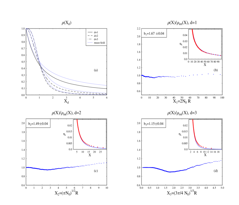
FIG. 2.: Residual density of impurities as a function of $X$. Fig. 2(a) shows the results of numerical computations for d=1,2,3 and the result of a simple mean field approximation Eq. (9). Fig. 2 (b)-(d) displays the ratio of $\rho_{d}$ as obtained by numerical computations to $\rho_{d}$ found using the interpolated formula Eq. (16) for $d$=1-3. The insets show the asymptotic behavior of the numerical data (triangles) and the interpolated formula (solid line).

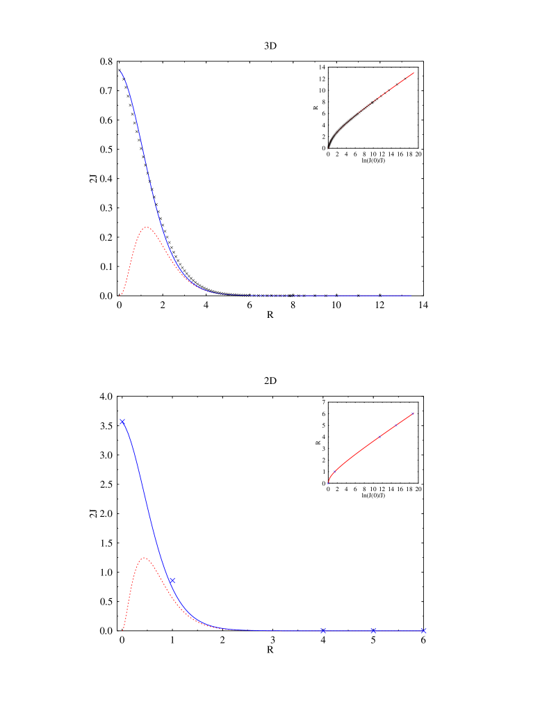
FIG. 3.: Interpolated formulae (solid lines) for $J(R)$ in the three- and two dimensional cases as given by Eqs. (22,29). For $3D$-case the crosses show numerical results of [18]. For $2D$-case the crosses show our numerical results at $R=1$ and and $R=0$. Dashed lines show the corresponding asymptotic formulae which are valid at large $R$. The solid lines in the insets show the behavior of the inverse function $R$ vs. $\ln(J(0)/J)$ as given by interpolated formulae (23) and (30). The crosses in the insets have the same meaning as in the main figures.

FIG. 4.: Dimensionless density of free spins $\rho(T)$ as a function of logarithm of temperature and dimensionless distribution function $F/n_{0}$ of the singlet-triplet excitations as a function of logarithm of energy in two-dimensional case (a),(b) and three-dimensional case (c), (d). The values of dimensionless density $\pi n_{0}a_{B}^{2}$ at (a) and (b) are 0.025 and 0.1. The values of dimensionless density $4\pi n_{0}a_{B}^{3}/3$ at (c) and (d) are 0.004 and 0.016. The solid lines show the final results of our calculations. The dashed lines show the results obtained with the function $J(R)$ as given by Eqs. (35). In all cases larger densities are shown by a thicker lines.

REFERENCES

- [1] e-mail: ilya@newt.phys.unsw.edu.au
- [2] B. I. Shklovskii, A. L. Efros, “Electronic properties of doped semiconductors”, Springer-Verlag, Berlin Heidelberg, 1984.
- [3] I. S. Shlimak, in Hopping and related Phenomena, edited by H. Fritzsche and Pollak (World Scientific, Singapore, 1990)
- [4] P. Dai, Y. Zhang, M. P. Sarachik, Phys. Rev. Lett. 69, 1804 (1992).
- [5] D. Simonian, S. V. Kravchenko, M. P. Sarachik, V. M. Pudalov, Phys. Rev. Lett., 79 , 2304 (1997).
- [6] S. Ishida, K. Oto, S, Takaoka, K. Murase, S. Shirai, and T. Serikawa, Phys. Stat. Sol. (b) 205,161 (1998).
- [7] I. S. Shlimak, S. I. Khondaker, J. T. Nicholls, M. Pepper, and D. A. Ritchie, unpublished.
- [8] K. M. Mertes, D. Simonian, S. V. Kravchenko, T. M. Klapwijk, preprint cond-mat/9903179.
- [9] M. Rosso, Phys. Rev. Lett., 44, 1541 (1980).
- [10] R. N. Bhatt, Phys. Rev. Lett., 48, 707 (1982).
- [11] R. N. Bhatt, P. A. Lee, J. Appl. Physics, 52, 1703 (1981).
- [12] K. Andres, R. N. Bhatt, P. Goalwin, T. M. Rice, and R. E. Walstedt, Phys. Rev. B 24, 244 (1981).
- [13] R. N. Bhatt, P. A. Lee, Phys. Rev. Lett., 48, 344 (1982).
- [14] P. A. Thomas, M. Rosso, Phys. Rev. B, 34, 7936 (1986).
- [15] R. N. Bhatt, D. S. Fisher, Phys. Rev. Lett., 68, 3072 (1992).
- [16] M. J. Hirsh, D. F. Holcomb, R. N. Bhatt, M. A. Paalanen, Phys. Rev. Lett., 68, 1418 (1992).
- [17] L. D. Landau and E. M. Lifshitz, “Quantum Mechanics”, Course of Theoretical Physics v. 3, Third Edition, Butterworth-Heinemann, Oxford, 1997, p. 240.
- [18] G. Staszewska and L. Wolniewicz, J. Mol. Specroscopy, 1999 (to be published); W. Kolos and L. Wolniewicz, Chem. Phys. Lett., 24, 457 (1974); L. Wolniewicz, JCP 99, 1851 (1993)
- [19] L. P. Gor’kov and L. P. Pitaevskii, Soviet Phys. Doklady, 8, 788 (1964); C.Herring and M. Flicker, Phys. Rev., 134, A362 (1964).
- [20] B. M. Smirnov and M. I. Chibisov, Soviet Phys. JETP, 21, 624 (1965).
- [21] V. V. Flambaum, I. V. Ponomarev, and O. P. Sushkov Phys. Rev. B, 59, 4163 (1999)
- [22] A. A. Radtsig and B. M. Smirnov, Parameters of Atoms and Atomic Ions, Energoatomizdat, Moscow, 1986.
- [23] A. L. Efros, V. V. Flambaum, and I. V. Ponomarev, unpublished
- [24] I. S. Grandshteyn and I. M. Ryzhik, Table of integrals, Series, and Products, Academic Press, Inc, 1980.
- [25] A. P. Prudnikov, et al., Integrals and Series, v.2, Nauka, Moskow, 1983.
- [26] H. A. Bethe and E. E. Salpeter, Quantum mechanics of one and two electron systems, Springer, Berlin, 1957.