Phase Separation under Shear in Two-dimensional Binary Fluids

Abstract

We use lattice Boltzmann simulations to study the effect of shear on the phase ordering of a two-dimensional binary fluid. The shear is imposed by generalising the lattice Boltzmann algorithm to include Lees-Edwards boundary conditions. We show how the interplay between the ordering effects of the spinodal decomposition and the disordering tendencies of the shear, which depends on the shear rate and the fluid viscosity, can lead to a state of dynamic equilibrium where domains are continually broken up and re-formed.

I Introduction

We present numerical results for the effect of shear flow on the spinodal decomposition of a two-dimensional binary fluid using lattice Boltzmann simulations. We show how the lattice Boltzmann algorithm can be generalised to allow the introduction of the Lees-Edwards boundary conditions, which are commonly used in molecular dynamics simulations to impose a shear flow without introducing walls. Results are presented showing how the competition between the ordering effects of the free energy and the disordering effects of the shear influences the spinodal decomposition and phase ordering of the fluid. For a recent review see Onuki [1].

When a binary fluid consisting of an equal amount of two components, A and B say, is rapidly cooled below the critical temperature it phase separates into an A-rich and B-rich phase. Once well-defined domains of each phase are formed the typical domain size grows according to a power law

$$R(t)\sim t^{\alpha}$$ (1)

where $\alpha$ is the growth exponent[2]. $\alpha$ depends on the growth mechanism, which is dictated by the surface tension, viscosity and diffusivity of the fluid, and the time elapsed after the quench. In two-dimensional systems diffusive Lifshitz-Slyozov growth gives $\alpha=\frac{1}{3}$ while hydrodynamics can lead to faster growth with $\alpha=\frac{2}{3}$.

The most obvious effect of shear flow on the domain growth is that the growing domains are elongated in the direction of the flow, leading to an anisotropic morphology. Experiments in three dimensions have shown that a string-like phase of thin domains oriented parallel to the shear can be formed in strong shear[3]. Such domains, which would normally be expected to be unstable due to the Rayleigh instability, appear to be stabilised by the shear, although very recent experiments show that they can eventually break up in strong shear [4].

This apparent stabilization suggests the possibility of a dynamic equilibrium when stretching and breaking of the domains as the result of the shear is balanced by their growth due to the thermodynamic driving force and to the coalescence of the domains, which can itself be driven by the shear. This was first proposed by Ohta and Nozaki [5] on the basis of two-dimensional simulations using a cell dynamic approach. These simulations, however, did not include hydrodynamics.

Simulations of phase separation under shear which include hydrodynamics are limited. Rothman performed early work using lattice gas cellular automata in two and three dimensions and was able to see the anisotropy of the growth [6, 7]. Wu et. al. undertook Langevin simulations in two and three dimensions and report the eventual formation of a string phase in three dimensions [8]. Padilla and Toxvaerd performed molecular dynamics simulations on a two-dimensional Lennard-Jones system, again pointing out the anisotropic nature of the domain growth [9]. In the simulations a peak was seen in the excess shear viscosity as a function of time corresponding to the increase in the lengths of interfaces in the system. However, there seems to be no evidence for a shear-induced dynamic equilibrium.

Here we simulate phase separation under shear using a lattice Boltzmann scheme in the same spirit as the model introduced by Orlandini et. al., which imposes phase separation by defining the fluid equilibrium as the minimum of an input free energy [10, 11]. This method has been very successful in obtaining results for phase separation in the absence of shear [12]. A particular advantage of the approach is that the fluid viscosity and diffusivity can be tuned, and this has allowed us to compare simulations for parameter values where diffusive or hydrodynamic phase separation dominates. We find either phases striped in the shear direction, or a dynamic equilibrium where the length scales remain approximately constant in time, depending on the relative strengths of the shear and the ordering.

The lattice Boltzmann approach is described in §2. Because this is a lattice rather than particulate simulation method, it is not immediately obvious how to define Lees-Edwards shear boundary conditions. An approach for doing this is given in §3. In particular it is necessary to generalize the normal definition of the lattice Boltzmann equilibrium distribution. In §4 we define suitable measures to characterise the anisotropic morphology of the spinodal decomposition patterns when shear is applied. The results of our simulations are contained in §5, where the effect of shear is compared for different fluid viscosities. §6 summarises the results and discusses outstanding questions.

II The Lattice Boltzmann Approach

The starting point for lattice Boltzmann simulations[13] is the evolution equation, discrete in space and time, for a set of distribution functions, ${f_{i}}$, each associated with a velocity vector, ${\bf v}_{i}$. For the sake of simplicity we consider a single relaxation time, the so-called BGK approximation [14]. The evolution equation for the $\{f_{i}\}$ is

$$f_{i}({\bf x}+{\bf v}_{i}\Delta t,t+\Delta t)-f_{i}({\bf x},t)=\frac{\Delta t}{\tau_{1}}(f_{i}^{0}-f_{i}),$$ (2)

where ${\bf x}$ is a lattice point, $\Delta t$ is the time step, and ${\bf v_{i}}\Delta t$ is normally constrained to be a lattice vector. The relaxation time is $\tau_{1}$ and $f_{i}^{0}$ is the equilibrium distribution. For a two-component system a second, equivalent equation is also needed

$$g_{i}({\bf x}+{\bf v}_{i}\Delta t,t+\Delta t)-g_{i}({\bf x},t)=\frac{\Delta t}{\tau_{2}}(g_{i}^{0}-g_{i}).$$ (3)

Physical quantities are defined as moments of the distribution functions. To model the isothermal flow of a binary mixture of components A and B, we choose

$$\sum_{i}f_{i}=n,\;\;\;\;\;\sum_{i}f_{i}{\bf v}_{i}=n{\bf u},\;\;\;\;\;\sum_{i}g_{i}=\varphi,$$ (4)

where $n$ is the total density field, ${\bf u}$ is the velocity field and $\varphi$ is the field corresponding to the difference in the density of components A and B.

We require mass conservation for both components and momentum conservation for the bulk. This is equivalent to constraining the equilibrium distributions to obey

$$\sum_{i}f_{i}^{0}=n,\;\;\;\;\;\sum_{i}g_{i}^{0}=\varphi,\;\;\;\;\;\sum_{i}f_{i}^{0}{\bf v}_{i}=n{\bf u}.$$ (5)

We also need to define higher-order moments of the equilibrium densities. The choice for these moments is within the free energy lattice Boltzmann scheme used here[10, 11]

$$\sum_{i}f_{i}^{0}v_{i\alpha}v_{i\beta} = P_{\alpha\beta}+nu_{\alpha}u_{\beta},$$ (6)

$$\sum_{i}g_{i}^{0}v_{i\alpha} = \varphi u_{\alpha},$$ (7)

$$\sum_{i}g_{i}^{0}v_{i\alpha}v_{i\beta} = \Gamma\mu\delta_{\alpha\beta}+\varphi u_{\alpha}u_{\beta},$$ (8)

where $P_{\alpha\beta}$ is the pressure tensor, $\Gamma$ is a mobility parameter, $\mu$ is the chemical potential for the density difference and $\delta$ is the Kronecker delta. The physical motivation for these constraints is twofold; firstly to ensure the correct form of the macroscopic equations of motion and secondly to reproduce the correct thermodynamics of the binary mixture in equilibrium as discussed in more detail below.

Taylor-expanding the evolution equations (2) and (3) to second order in the derivatives gives the macroscopic equations of motion for the binary fluid[15]. These are the continuity equation for the total density

$$\partial_{t}n+\partial_{\alpha}nu_{\alpha}=0,$$ (9)

a convection-diffusion equation governing the evolution of the density difference

$$\partial_{t}\varphi+\partial_{\alpha}(\varphi u_{\alpha})=\omega_{2}\left(\Gamma\nabla^{2}\mu-\partial_{\beta}\left(\frac{\varphi}{n}\partial_{\alpha}P_{\alpha\beta}\right)\right),$$ (10)

and, in the incompressible limit, the incompressible Navier Stokes equations for a non-ideal system

$$n\partial_{t}u_{\alpha}+nu_{\beta}\partial_{\beta}u_{\alpha}=-\partial_{\beta}P_{\alpha\beta}+\frac{n\omega_{1}}{3}\nabla^{2}u_{\alpha}+O(\partial^{3})$$ (11)

where $\omega_{1,2}=\tau_{1,2}-\Delta t/2$ and the viscosity is given by $\nu=n\omega_{1}/3$.

The thermodynamic fields entering the simulation are the pressure tensor and the chemical potential which follow from the free energy of the system. We consider the free energy of a simple binary fluid. A–A and B–B interactions are zero, but there is an A–B repulsion $\lambda n_{A}n_{B}$ where $n_{A}$ and $n_{B}$ are the number densities of A- and B-particles, respectively, and $\lambda$ is a parameter describing the interaction strength. This system can be described by the Landau free energy functional

$$\Psi=\int d{\bf r}\left\{\psi(\varphi,n,T)+\frac{\kappa}{2}(\nabla\varphi)^{2}\right\}$$ (12)

where $T$ is the temperature and $\kappa$ is a measure of the excess interface free energy (surface tension). The free energy density of the homogeneous system is [16]

$$\psi(\varphi,n,T) = \frac{\lambda n}{4}\left(1-\frac{\varphi^{2}}{n^{2}}\right)-Tn$$ (15)

$$+\frac{T}{2}(n+\varphi)\ln\left(\frac{n+\varphi}{2}\right)$$

$$+\frac{T}{2}(n-\varphi)\ln\left(\frac{n-\varphi}{2}\right).$$

For temperatures greater than a critical temperature $T_{c}=\lambda/2$ the system remains in a single phase. For $T<T_{c}$ there is phase separation into two states with $\varphi=\pm\varphi_{0}$.

From the free energy (12) we derive the local chemical potential $\mu$ as the functional derivative of the total free energy $\Psi$ with respect to the concentration difference field $\varphi({\bf x})$

$$\mu({\bf x})=\frac{\delta\Psi}{\delta\varphi({\bf x})}=-\frac{\lambda}{2}\frac{\varphi}{n}+\frac{T}{2}\ln\left(\frac{n+\varphi}{n-\varphi}\right)-\kappa\nabla^{2}\varphi.$$ (16)

Equilibrium corresponds to $\mu(\phi,n,T)=0$.

The derivation of the pressure tensor is slightly more involved and is discussed in Appendix A[17]. We obtain

$$P_{\alpha\beta} = (n\partial_{n}\psi+\varphi\partial_{\varphi}\psi-\psi)\delta_{\alpha\beta}$$ (18)

$$+\kappa(\partial_{\alpha}\varphi\partial_{\beta}\varphi-\frac{1}{2}\partial_{\gamma}\varphi\partial_{\gamma}\varphi\delta_{\alpha\beta}-\varphi\partial_{\gamma}\partial_{\gamma}\varphi)$$

$$= (nT+\varphi\mu^{0}(x))\delta_{\alpha\beta}$$ (20)

$$+\kappa(\partial_{\alpha}\varphi\partial_{\beta}\varphi-\frac{1}{2}\partial_{\gamma}\varphi\partial_{\gamma}\varphi\delta_{\alpha\beta}-\varphi\partial_{\gamma}\partial_{\gamma}\varphi)$$

$$= (nT+\varphi\mu(x))\delta_{\alpha\beta}$$ (22)

$$+\kappa(\partial_{\alpha}\varphi\partial_{\beta}\varphi-\frac{1}{2}\partial_{\gamma}\varphi\partial_{\gamma}\varphi\delta_{\alpha\beta})$$

where the first term is the ideal gas pressure, the second term is the osmotic pressure with $\mu^{0}=\partial_{\phi}\psi$ and the third term is related to the surface tension. The osmotic pressure was omitted in the original definition of the model [10, 11]. The chemical potential and pressure tensor are input to the lattice Boltzmann scheme through equations (6) and (8). In equilibrium the simulated fluid minimises the free energy (12).

It remains only to define the equilibrium distributions $f_{i}^{0}$ and $g_{i}^{0}$ introduced in the evolution equations (2) and (3). Normally an expansion to second order in the velocities is sufficient to reproduce the constraints (5) – (8)[13]. However, this ceases to be the case when Lees-Edwards shear boundary conditions are introduced. In the next section we discuss how the equilibrium distribution can be defined to allow the use of Lees-Edwards boundary conditions.

III Shear boundary conditions

Possibly the easiest way to introduce shear flow in a lattice Boltzmann simulation is to include walls moving in a lattice direction. Even for a wall with neutral wetting, however, phase separation is strongly enhanced at the walls and the wall effects easily dominate the phase separation process for all but the largest systems. The effect of walls on phase separation is an interesting phenomenon in its own right, but it is not the process we are interested in studying here.

The problem caused by explicit walls can be overcome in a relatively simple and efficient manner by introducing a Klein-bottle symmetry to the lattice. This is done by forcing the fluid to have a given velocity along one line in the direction of the shear flow. In a one-component mixture this induces a linear velocity profile. For a two-component mixture, however, the dynamics are influenced by the V-shaped velocity profile at the forcing line because of the non-local interactions. We used this algorithm to produce preliminary results but it has no advantages over the method derived below.

A more regular shear flow can be produced by extending the idea of Lees-Edwards boundary conditions, widely used in Molecular Dynamics [18], to lattice Boltzmann simulations. Briefly, Lees and Edwards simulated shear boundary conditions for a shear in the $x$-direction in a simulation box of dimensions $(X,Y)$ by introducing periodic boundary conditions in the $y$-direction. Particles that left the box at the lower boundary for position $(x,y=0)$ reappeared at the upper boundary at position $(x+ut(\bmod X),y=Y)$ with a velocity that was changed by $v\rightarrow v+u$.

To implement this idea for lattice Boltzmann simulations we are faced with two difficulties. Firstly the densities are defined on a lattice and the Lees-Edwards boundary conditions lead to densities defined between the lattice points. Secondly we need to impose a Galilean transformation for the densities which are streamed across the lattice.

The non-fitting of the lattice is relevant for both the streaming and for the calculation of derivatives at $y=1$ and $y=Y$. We solve this problem by a linear interpolation scheme. For any density we define

$$f[x,y=0] = (1-R(ut))f[x+I(ut),y=Y]$$ (24)

$$+R(ut)f[x+I(ut)+1,y=Y]$$

where $I(z)$ is the largest integer with $I(z)<z$ and $R(z)=z-I(z)$. If we pass the break in the lattice from the other side we define similarly

$$f[x,y=Y+1] = (1-R(ut))f[x-I(ut),y=1]$$ (26)

$$+R(ut)f[x-I(ut)-1,y=1].$$

These formulae are used both for the streaming of the Galilean-transformed Boltzmann densities, $f_{i}$, and for the calculation of density gradients.

FIG. 1.: Our numbering of the velocity vectors in a nine-velocity model.

It is rather more difficult to see how the Galilean transformation should be defined. Let us consider the special case of a two-dimensional, nine-velocity model where the velocities are numbered as indicated in Figure 1. We need to perform a Galilean transformation on the $\{5,2,6\}$ and the $\{7,4,8\}$ velocities as these will carry mass and momentum across the boundaries. To define the transformation we demand mass and $y$-momentum conservation

$$n_{p}\equiv f_{5}+f_{2}+f_{6}=f_{5}^{\prime}+f_{2}^{\prime}+f_{6}^{\prime}$$ (27)

an appropriate change in the $x$-momentum

$$(f_{5}-f_{6})-(f^{\prime}_{5}-f^{\prime}_{6})=n_{p}u$$ (28)

and conservation of the local pressure

$$P^{p}_{xx} = \sum{\frac{f_{i}}{{n_{p}}^{2}}(n{v_{i}}_{x}-n_{p}u_{x})^{2}}$$ (29)

$$= \frac{1}{{n_{p}}^{2}}\left((f_{5}(n_{p}-n_{p}u_{x})^{2}+f_{2}(n_{p}u_{x})^{2}\right.$$ (31)

$$\left.+f_{6}(-n_{p}-n_{p}u_{x})^{2}\right)$$

$$= \frac{1}{{n_{p}}^{2}}\left(f_{5}^{\prime}(n_{p}-n_{p}u_{x}^{\prime})^{2}+f_{2}^{\prime}(n_{p}u_{x}^{\prime})^{2}\right.$$ (33)

$$\left.+f_{6}^{\prime}(-n_{p}-n_{p}u_{x}^{\prime})^{2}\right)$$

where the prime denotes the transformed quantities.

This system of equations can be solved to give a unique solution for the Galilean-transformed densities $f_{i}^{\prime}$

$$f_{2}^{\prime} = f_{2}+2(f_{5}-f_{6})u-n_{p}u^{2},$$ (34)

$$f_{5}^{\prime} = f_{5}+(-\frac{3}{2}f_{5}-\frac{1}{2}f_{2}+\frac{1}{2}f_{6})u+\frac{n_{p}}{2}u^{2},$$ (35)

$$f_{6}^{\prime} = f_{6}+(-\frac{1}{2}f_{5}+\frac{1}{2}f_{2}+\frac{3}{2}f_{6})u+\frac{n_{p}}{2}u^{2}.$$ (36)

This definition can be extended to a Galilean transformation for all densities and, equivalently, to a transformation in different lattice directions.

In order for this transformation to make sense we need to make sure that equation (28) is consistent with the definition of the equilibrium distribution, $f_{i}^{0}$ in Eqn. (2) i.e. that an equilibrium distribution for a velocity $u$ Galilean transformed by a velocity $\Delta u$ is equal to the equilibrium distribution for velocity $u+\Delta u$. It is conventional to define the equilibrium distribution as a polynomial in second order in u. A generic expansion is

$$f_{i}^{0} = A_{\sigma}n+B_{\sigma}nu_{\alpha}{v_{i}}_{\alpha}+C_{\sigma}nu^{2}$$ (38)

$$+D_{\sigma}nu_{\alpha}u_{\beta}{v_{i}}_{\alpha}{v_{i}}_{\beta}+G_{\sigma\alpha\beta}n{v_{i}}_{\alpha}{v_{i}}_{\beta}$$

where $A_{\sigma},B_{\sigma},C_{\sigma},D_{\sigma},G_{\sigma\alpha\beta}$ are constants that have the absolute value of the corresponding velocity vector $\sigma=|{\bf v}_{i}|$ as an index. However, substituting (38) into (28) shows that this equation is not satisfied in equilibrium. In practice this leads to a step in the $u_{x}$ profile at the boundary.

There is, however, no a priori reason to use a second-order expansion in the velocity for the equilibrium distribution. All that is needed for a valid equilibrium distribution is that (5)–(8) hold and that the distribution obeys the conditions (34)–(36).

Let $T_{\alpha\beta}=P_{\alpha\beta}/n$. Then, if we require,

$$\frac{f^{0}_{1}-f^{0}_{3}}{f^{0}_{1}+f^{0}_{0}+f^{0}_{3}}=u_{x},\;\;\;\;\;\;\;\;\;\;\;\frac{f^{0}_{2}-f^{0}_{4}}{f^{0}_{2}+f^{0}_{0}+f^{0}_{4}}=u_{y}$$ (39)

$$f^{0}_{5}+f^{0}_{6}-(f^{0}_{5}+f^{0}_{6}+f^{0}_{2})(T_{xx}+u_{x}u_{x})=0,$$ (40)

$$f^{0}_{5}+f^{0}_{8}-(f^{0}_{5}+f^{0}_{8}+f^{0}_{1})(T_{yy}+u_{y}u_{y})=0,$$ (41)

$$f^{0}_{8}+f^{0}_{7}-(f^{0}_{8}+f^{0}_{7}+f^{0}_{4})(T_{xx}+u_{x}u_{x})=0,$$ (42)

$$f^{0}_{6}+f^{0}_{7}-(f^{0}_{6}+f^{0}_{7}+f^{0}_{3})(T_{yy}+u_{y}u_{y})=0.$$ (43)

(39)-(43), together with (5)–(8) are a completely determined set of equations with the solution

$$f^{0}_{0} = n(1-T_{xx}-u_{x}^{2})(1-T_{yy}-u_{y}^{2}),$$ (44)

$$f^{0}_{1} = \frac{1}{2}n(T_{xx}+u_{x}+u_{x}^{2})(1-T_{yy}-u_{y}^{2}),$$ (45)

$$f^{0}_{2} = \frac{1}{2}n(T_{yy}+u_{y}+u_{y}^{2})(1-T_{xx}-u_{x}^{2}),$$ (46)

$$f^{0}_{3} = \frac{1}{2}n(T_{xx}-u_{x}+u_{x}^{2})(1-T_{yy}-u_{y}^{2}),$$ (47)

$$f^{0}_{4} = \frac{1}{2}n(T_{yy}-u_{y}+u_{y}^{2})(1-T_{xx}-u_{x}^{2}),$$ (48)

$$f^{0}_{5} = \frac{1}{4}n(T_{xy}+T_{xx}T_{yy}+T_{yy}(u_{x}+u_{x}^{2})$$ (50)

$$+T_{xx}(u_{y}+u_{y}^{2})+u_{x}u_{y}(1+u_{x}+u_{y}+u_{x}u_{y})),$$

$$f^{0}_{6} = \frac{1}{4}n(-T_{xy}+T_{xx}T_{yy}+T_{yy}(-u_{x}+u_{x}^{2})$$ (52)

$$+T_{xx}(u_{y}+u_{y}^{2})-u_{x}u_{y}(1-u_{x}+u_{y}-u_{x}u_{y})),$$

$$f^{0}_{7} = \frac{1}{4}n(T_{xy}+T_{xx}T_{yy}+T_{yy}(-u_{x}+u_{x}^{2})$$ (54)

$$+T_{xx}(-u_{y}+u_{y}^{2})+u_{x}u_{y}(1-u_{x}-u_{y}+u_{x}u_{y})),$$

$$f^{0}_{8} = \frac{1}{4}n(-T_{xy}+T_{xx}T_{yy}+T_{yy}(u_{x}+u_{x}^{2})$$ (56)

$$+T_{xx}(-u_{y}+u_{y}^{2})-u_{x}u_{y}(1+u_{x}-u_{y}-u_{x}u_{y})).$$

For this equilibrium distribution

$$\frac{f^{0}_{5}-f^{0}_{6}}{f^{0}_{5}+f^{0}_{2}+f^{0}_{6}}=u_{x}+\frac{T_{xy}}{T_{yy}+u_{y}+u_{y}^{2}}$$ (57)

which is consistent with the Galilean transformation (28).

For a two-component system we similarly define the $g_{i}^{0}$ using

$$\frac{g^{0}_{1}-g^{0}_{3}}{g^{0}_{1}+g^{0}_{0}+g^{0}_{3}}=u_{x},\;\;\;\;\;\;\;\;\;\frac{g^{0}_{2}-g^{0}_{4}}{g^{0}_{2}+g^{0}_{0}+g^{0}_{4}}=u_{y}$$ (58)

and imposing

$$g_{0}=\varphi-\ell\Gamma\mu-\varphi(u_{x}^{2}+u_{y}^{2})$$ (59)

where $\ell$ is a free parameter that can be used to improve stability (we choose $\ell=1$). Solving equations (58) and (59) and (5)–(8) gives

$$g^{0}_{1} = 1/2\{(\ell-1-u_{x})\Gamma\mu+(1+u_{x}-u_{y}^{2})\varphi u_{x}\},$$ (60)

$$g^{0}_{2} = 1/2\{(\ell-1-u_{y})\Gamma\mu+(1+u_{y}-u_{x}^{2})\varphi u_{y}\},$$ (61)

$$g^{0}_{3} = 1/2\{(\ell-1+u_{x})\Gamma\mu-(1-u_{x}-u_{y}^{2})\varphi u_{x}\},$$ (62)

$$g^{0}_{4} = 1/2\{(\ell-1+u_{y})\Gamma\mu-(1-u_{y}-u_{x}^{2})\varphi u_{y}\},$$ (63)

$$g^{0}_{5} = 1/4\{(2-\ell+u_{x}+u_{y})\Gamma\mu+(1+u_{x}+u_{y})\varphi u_{x}u_{y}\},$$ (64)

$$g^{0}_{6} = 1/4\{(2-\ell-u_{x}+u_{y})\Gamma\mu-(1-u_{x}+u_{y})\varphi u_{x}u_{y}\},$$ (65)

$$g^{0}_{7} = 1/4\{(2-\ell-u_{x}-u_{y})\Gamma\mu+(1-u_{x}-u_{y})\varphi u_{x}u_{y}\},$$ (66)

$$g^{0}_{8} = 1/4\{(2-\ell+u_{x}-u_{y})\Gamma\mu-(1+u_{x}-u_{y})\varphi u_{x}u_{y}\}.$$ (67)

The macroscopic flow equations are unaffected by the choice of the further constraints (39)–(43) and (58)–(59) or by the detailed structure of the equilibrium distributions. Therefore, these alterations in the model can change the numerical stability and the behaviour of quantities like the spurious velocities, but they leave the evolution of the macroscopic quantities unaffected, at least to second order in the derivatives.

IV Measures for non-isotropic patterns

To characterise the features of phase separation under shear it is necessary to construct measures for the length scales of the sheared systems which will in general be anisotropic. Measures that are based on Fourier transforms cannot be easily used for sheared systems because the system is no longer periodic.

Length scales derived from derivatives do not require periodicity. Derivatives need to be evaluated for the algorithm and are readily available. We define a tensor

$$d_{\alpha\beta}=\frac{\sum_{\bf x}\partial_{\alpha}^{D}\varphi({\bf x},t)\partial_{\beta}^{D}\varphi({\bf x},t)}{\sum_{\bf x}\varphi^{2}({\bf x},t)}$$ (68)

where $\partial_{\alpha}^{D}$ is the symmetric discrete derivative in direction $\alpha$. Because the tensor is symmetric it can be diagonalised to give two eigenvalues $\lambda_{1},\lambda_{2}$ and an angle $\theta^{\star}$

$$\lambda_{1} = \frac{d_{xx}+d_{yy}}{2}+\sqrt{\frac{(d_{xx}-d_{yy})^{2}}{4}+d_{xy}^{2}},$$ (69)

$$\lambda_{2} = \frac{d_{xx}+d_{yy}}{2}-\sqrt{\frac{(d_{xx}-d_{yy})^{2}}{4}+d_{xy}^{2}},$$ (70)

$$\theta^{\star} = \tan^{-1}\left(\frac{d_{yy}}{d_{xy}-\lambda_{2}}\right).$$ (71)

The two eigenvalues give two orthogonal length scales

$$R^{\star}_{1}(t)=\frac{1}{\lambda_{1}(t)L_{w}},\;\;\;\;\;\;\;\;R^{\star}_{2}(t)=\frac{1}{\lambda_{2}(t)L_{w}},$$ (72)

where $L_{w}$ is the interface width. It appears because $d_{\alpha\beta}$ scales inversely with the interface width[15]. $L_{w}$, used as a constant here, could in principle be anisotropic. That this anisotropy is not a strong effect can be seen by comparing these length scales with scales that are explicitly independent of the interface width.

One such measure is related to the lengths of the interfaces in the system. The interface can be represented by a set of contours. These contours consist of small line segments $\vec{l}_{i}$ and the length of the interface can be written

$$L_{I}=\sum_{i}|\vec{l}_{i}|.$$ (73)

In order to extract the preferred direction of the interface we define the vector

$$\vec{D}=R^{-1}\left(\sum_{i}R(\vec{l}_{i})\right).$$ (74)

The operator $R$ is defined by

$$R(\vec{x})=|\vec{x}|\left(\begin{array}[]{c}\cos(2\theta)\\ \sin(2\theta)\end{array}\right)$$ (75)

where $\theta$ is the angle between the argument of R and the $x$-axis.

$\vec{D}$ is a vector that is zero for isotropic closed contours and which points in the average direction of the interface for non-isotropic closed contours. Two length scales and an angle that correspond to the intuitive result for oriented rectangular objects can be defined from these measures

$$R^{\circ}_{1}=\frac{XY}{L_{I}+|\vec{D}|},\;\;\;\;\;\;\;\;R^{\circ}_{2}=\frac{XY}{L_{I}-|\vec{D}|},$$ (76)

$$\theta^{\circ}=\cos^{-1}\left(\frac{\hat{\vec{x}}.\vec{D}}{|\vec{D}|}\right).$$ (77)

Thus we have defined two independent sets of measures for the structure of non-isotropic patterns that will now be used to examine spinodal decomposition under shear.

V Simulation results

For all the simulations we used a total density $n=2$, an interaction parameter $\lambda=1.1$, which corresponds to a critical temperature $T_{c}=0.55$, and a temperature $T=0.5$. The equilibrium values of the order parameter were then $\varphi_{0}=\pm 1$. The mobility was $\Gamma=2$, the relaxation time for the order parameter in Eqn. (3) was $\tau_{2}=1$ and the interface free energy parameter was $\kappa=0.002$, which corresponds to an interface width of approximately three lattice spacings. The relaxation parameter for the total density Eqn. (2), $\tau_{1}$, was varied: $\tau_{1}=100$ gave a high viscosity and $\tau_{1}=1$ an intermediate viscosity.

The shear transformation, S, is defined as

$$S\left(\begin{array}[]{c}x\\ y\end{array}\right)=\left(\begin{array}[]{r}x+\dot{\gamma}ty\\ y\end{array}\right).$$ (78)

Shear flow applied to a system undergoing spinodal decomposition stretches the original pattern. This effect is only relevant once the deformation caused by the flow is of the same order or larger than the deformation caused by the coarsening process. This requires

$$\dot{\gamma}t>1.$$ (79)

We therefore expect to observe the effect of the shear flow for $t>1/\dot{\gamma}$.

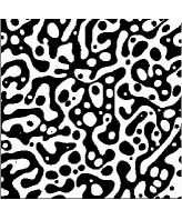
time=0

time=1

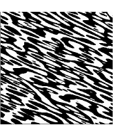
time=2

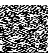
time=3

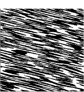
time=4

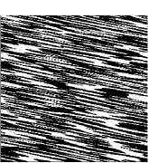
time=5

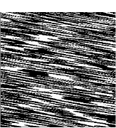
time=6

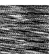
time=10

FIG. 2.: Applying shear (with shear rate $\dot{\gamma}=1$) to a system without internal dynamics leads to homogenization.

To help understand the effect of shear-flow on a phase-separating system let us first consider a pattern without any internal dynamics that undergoes a shear transformation. This transformation is illustrated in Figure 2, where we start from a frozen spinodal decomposition pattern and show successive iterations of a shear transformation with $\dot{\gamma}=1$.

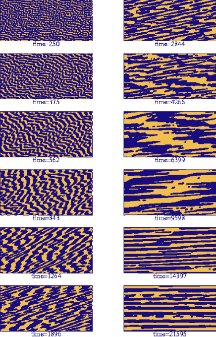
(a)

$\mbox{}\;\;\theta^{*}$

$\mbox{}\;\;\theta^{\circ}$

time

(b)

$R^{*}_{1,2}$

$R^{\circ}_{1,2}$

time

(c)

FIG. 3.: (a) Spinodal decomposition under shear for a high viscosity binary fluid $(\tau_{1}=100,L_{x}=256,L_{y}=128)$. The high viscosity suppresses internal hydrodynamic degrees of freedom. The shear rate is $\dot{\gamma}=0.004$ which corresponds to a shear time $t_{s}=250$. (b) Variation of the orientation (in degrees) of the pattern with time. (c) Variation of the length scales (in arbirtary units) with time.

The structure develops an orientation that slowly aligns with the shear direction while the stretching increases the length of the domains along the shear. Once the width of the domains is smaller than the original width of the interface the system is effectively a homogeneous mixture.

This effect is known as shear-induced mixing. It can be observed in the lattice Boltzmann fluids if the stretching effect of the shear flow is much faster than the growth of the domains via diffusion or flow. Numerically this can be achieved by choosing a very low mobility and a high viscosity. Phase separation is suppressed because of the mixing properties of the shear flow unless the phase-separating structure is aligned with the shear direction. For finite lattices we sometimes observe at much later times a nucleation of complete stripes that span the system and are periodic in the shear direction. The time required to form these stripes depends on the system size and it seems reasonable to assume that this phenomenon does not occur in infinite systems.

We now consider a high viscosity fluid ($\tau_{1}=100$) in which diffusive but not hydrodynamic modes are important. The internal dynamics leads to domain coarsening and can also prevent a complete mixing of the system. Figure 3 shows the spinodal decomposition pattern of the high-viscosity binary mixture. For very short times ($t<300\sim\dot{\gamma}^{-1}$) we observe the familiar spinodal decomposition pattern. It is, however, coarsening in a new way via shear flow-induced collisions of the domains. This process enhances domains oriented in the collision direction. Then for $300<t<1000$ the flow slowly turns the striped pattern and stretches it. At $t\sim 1000$ the rupturing of domains starts to be important and for $1000<t<15000$ there is a continuous stretching and rupturing that effectively stops the phase ordering process. At $t\sim 15000$ the system developes stripes that span the system. Because periodic stripes are unaffected by the shear flow if they are completely aligned with it the system now grows via the diffusion mechanism.

This evolution can be followed more quantitatively by measuring the orientation angle and the length scales defined in Section IV. Figure 3b shows the angle of orientation to the $x$-axis measured by $\theta^{\star}$ (Eqn. 71) and $\theta^{\circ}$ (Eqn. 77). The two different measures for the angle agree very well. The pattern tilts at very early times ($t<2000$) and then slowly aligns with the direction of the shear flow as periodic stripes are created.

The graph in Figure 3c shows the length-scales $R_{1,2}^{\star}$ defined in Eqns. (72) and the length scales $R_{1,2}^{\circ}$ defined in Eqns. (76). We very clearly see a separation of length scales and a good agreement of the two different measures. A minimum of the larger length scale at $t\sim 17000$ indicates the creation of periodic stripes spanning the system. After this time the growth of domains is no longer hindered by the continual breaking of stretched domains.

We now turn to consider a system with a lower viscosity that allows for a hydrodynamic response of the domains to the shear flow. Results are presented in Figure 4. It is immediately obvious that the pattern differs

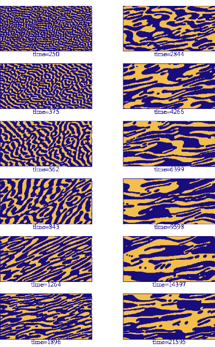
(a)

$\mbox{}\;\;\;\theta^{*}$

$\mbox{}\;\;\;\theta^{\circ}$

time

(b)

$R^{*}_{1,2}$

$R^{\circ}_{1,2}$

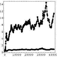
time

(c)

FIG. 4.: (a) Spinodal decomposition under shear for a medium viscosity binary fluid $(\tau_{1}=1,L_{x}=256,L_{y}=128)$. The effect of internal flow causes the domains to remain at an angle to the shear direction. The shear rate is $\dot{\gamma}=0.004$ which corresponds to a shear time $t_{s}=250$. (b) Variation of the orientation (in degrees) of the pattern with time. (c) Variation of the length scales (in arbitrary units) with time.

from that in Figure 3. The final state does not simply consist of periodic stripes, but of dynamic structures that are constantly stretched, broken and deformed by the flow. At least on this time scale a state of dynamic equilibrium is reached where the ordering effects of the spinodal decomposition balance the disordering effects of the shear.

The quantitative measures in Figures 4b and 4c show that after initial fluctuations the orientation of the pattern converges to a value that fluctuates about a finite angle to the shear direction. This phenomenon is similar to the behaviour of a single sheared drop that lies at a finite angle to a shear flow[19]. The graph of length scales again shows a very clear distinction between the large and small length scales. Strong oscillations are seen. These may be finite size effects because the system is so small and contains only a few domains. However such oscillations have been seen in experiments [4] and ina model system [20].

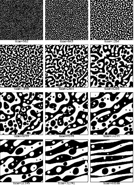
(a)

$\mbox{}\;\;\theta^{*}$

$\mbox{}\;\;\theta^{\circ}$

time

(b)

$R^{*}_{1,2}$

$R^{\circ}_{1,2}$

time

(c)

FIG. 5.: (a) Spinodal decomposition under shear for a high viscosity binary fluid $(\tau_{1}=100,L_{x}=512,L_{y}=512)$. The high viscosity suppresses internal hydrodynamic degrees of freedom. The shear rate is $\dot{\gamma}=0.0001$ which corresponds to a shear time $t_{s}=1000$. (b) Variation of the orientation (in degrees) of the pattern with time. (c) Variation of the length scales (in arbitrary units) with time.

We have, so far, considered strong shear flow. Let us now consider the same viscosity, where both diffusive and hydrodynamic flow is possible, but lower the shear rate so that the early time spinodal decomposition is unaffected by the flow. In Figure 5 the spinodal decomposition for a shear rate $\dot{\gamma}=0.0001$ is shown for a system with $\tau_{1}=1$. For times $t<1/\dot{\gamma}=10000$ we see the typical spinodal decomposition pattern for these viscosities. Hydrodynamic flow leads to circular domains which then grow through the slower diffusive mechanism. After this time, the stretching of the domains dominates over the domain growth and the pattern becomes non-isotropic. By $t\sim 10000$ the pattern comprises large-stripe like domains together with the nested pattern of drops within drops in the large domains. As the large domains are stretched, the drops inside them coalesce with the walls and slowly the stripes are cleaned of the small included drops.

These results also clearly show up in the measurements given in Figure 5. After $t>10000$ the orientation slowly converges towards a tilting angle $\theta\sim 7^{\circ}$, the long and short length scales split and the $R^{\star}\sim R^{\circ}\sim R^{1}\sim t^{\frac{2}{3}}$ growth law breaks down. In the $R^{\#}$ measure derived from the number of domains we see a slight increase from the normal growth law corresponding to the process of shear cleaning the stripes from drops.

VI Conclusions

In this paper we have investigated the effects of shear flow on systems undergoing spinodal decomposition. In order to study these systems we introduced an extension to the lattice Boltzmann algorithm that allows simulation of shear flow problems with Lees-Edwards boundary conditions. We find that the effect of shear flow on spinodal decomposition depends strongly on the viscosity of the fluid. Systems with a very high viscosity tend to order in the shear direction, whereas systems with a lower viscosity arrive at a dynamic stationary state where the domains lie at a finite angle to the shear direction.

One of the problems in simulating spinodal decomposition under shear is that the shear flow induces long-range correlations much faster than for un-sheared systems so that larger lattice sizes are required to examine long-time behaviour. Therefore there remain many unexplored problems concerning the structure of spinodal decomposition under shear. For example, it would be interesting to investigate the transition between the sheared and non-sheared patterns for different viscosities and to ask whether the late-time decomposition patterns are statistically independent of an initial shear.

Appendix A

We show how the full pressure tensor (22) is derived. The pressure of a homogeneous system is defined as the volume derivative of the free energy. Writing the full volume dependence of the densities $n=N/V$ and $\varphi=(N_{A}-N_{B})/V$ explicitly we see that:

$$P = -\partial_{V}\int_{V}\psi\left(\frac{N}{V},\frac{N_{A}-N_{B}}{V}\right)$$ (80)

$$= -\partial_{V}\left(V\psi\left(\frac{N}{V},\frac{N_{A}-N_{B}}{V}\right)\right)$$ (81)

$$= n\partial_{n}\psi+\varphi\partial_{\varphi}\psi-\psi.$$ (82)

For a non-homogeneous system the pressure is no longer a scalar but a tensor. The correct form of the pressure tensor can be derived from a Lagrangian expression for the free energy which is minimized in equilibrium

$$L = \int_{V}\left(\psi(n,\varphi)+\frac{\kappa}{2}\partial_{\alpha}\varphi\partial_{\alpha}\varphi\right)$$ (84)

$$+\mu_{\varphi}(\int_{V}\varphi-(N_{A}-N_{B}))+\mu_{n}(\int_{V}n-N).$$

To obtain differential equations for the equilibrium we evaluate the Euler-Lagrange equations and get

$$\mu_{\varphi} = -\partial_{\varphi}\psi+\kappa\partial_{\alpha}\partial_{\alpha}\varphi,$$ (85)

$$\mu_{n} = -\partial_{n}\psi.$$ (86)

We multiply these equations with $\partial_{\beta}\varphi$ and $\partial_{\beta}n$, respectively and sum the equations. Remembering that $\mu_{\varphi}$ and $\mu_{n}$ are constants, this yields

$$\partial_{\beta}(\varphi\mu_{\varphi}+n\mu_{n}) = -\partial_{\alpha}(\psi\delta_{\alpha\beta}$$ (88)

$$+\kappa\{\partial_{\alpha}\varphi\partial_{\beta}\varphi-\frac{1}{2}\partial_{\gamma}\varphi\partial_{\gamma}\varphi\delta_{\alpha\beta})\}.$$

We then substitute the expressions for the chemical potentials (47) and (48) into (88) and subtract the right-hand side from the left-hand side to derive a tensor $\sigma$ that has a zero divergence

$$\partial_{\alpha}\sigma_{\alpha\beta} = \partial_{\alpha}((\varphi\partial_{\varphi}\psi+n\partial_{n}\psi-\psi)\delta_{\alpha\beta}$$ (90)

$$+\kappa(\partial_{\alpha}\varphi\partial_{\beta}\varphi-\frac{1}{2}\partial_{\gamma}\varphi\partial_{\gamma}\varphi\delta_{\alpha\beta}-\varphi\partial_{\gamma}\partial_{\gamma}\varphi\delta_{\alpha\beta})).$$

For a uniform system $\sigma_{\alpha\beta}=P\delta_{\alpha\beta}$ reduces to the homogeneous pressure. The divergence of the pressure tensor must vanish in equilibrium. We therefore identify $\sigma_{\alpha\beta}$ with the pressure tensor $P_{\alpha\beta}$.

. .

REFERENCES

• [1] A. Onuki, J. Phys. Cond. Mat. 9, 6119 (1997)
• [2] A.J. Bray, Adv. Phys. 43, 357 (1994)
• [3] T. Hashimoto, K. Matsuzaka, E. Moses and A. Onuki, Phys. Rev. Lett. 74, 126 (1995)
• [4] K. Matsuzaka, T. Koga and T. Hashimoto, Phys. Rev. Lett. 80, 5441 (1998)
• [5] T. Ohta, H. Nozaki and M. Doi, Phys. Lett. A 145, 304 (1990)
• [6] J.F. Olson and D.H. Rothman, J. Stat. Phys. 81, 199 (1995)
• [7] D.H. Rothman, Europhys. Let. 14, 337 (1991)
• [8] Y.N. Wu, H. Skrdla, T. Lookman and S.Y. Chen, Physica A 239, 428 (1997)
• [9] P. Padilla and S. Toxvaerd, J. Chem. Phys. 106, 2342 (1997)
• [10] E. Orlandini, M.R. Swift and J.M. Yeomans, Europhys. Let. 32, 463 (1995)
• [11] M.R. Swift, E. Orlandini, W.R. Osborn and J.M. Yeomans, Phys. Rev. E 54, 5041 (1996)
• [12] A. Wagner and J.M. Yeomans, Phys. Rev. Lett. 80, 1429 (1998)
• [13] S. Chen and G.D. Doolen, An. Rev. Fl. Mech. 30, 329 (1998)
• [14] Y.H. Qian, D. dโ€™Humiรจres and P. Lallemand, Europhys. Let. 17, 479 (1992)
• [15] A. Wagner, D. Phil. thesis, University of Oxford, (1997).
• [16] L.E. Reichl, A modern course in statistical Physics, Edward Arnold, London (1980)
• [17] A.J.M. Yang, P.D. Fleming and J.H. Gibbs, J. Chem. Phys. 64, 3732 (1976)
• [18] A.W. Lees and S.F. Edwards, J. Phys. C 5, 1921 (1972)
• [19] H.A. Stone, An. Rev. Fl. Mech. 26, 65 (1994)
• [20] F. Corberi, G. Gonella and A. Lamura, cond-mat/9806239