Critical dynamics of a uniaxial and dipolar ferromagnet

Abstract

We study the critical dynamics of three-dimensional ferromagnets with uniaxial anisotropy by taking into account exchange and dipole-dipole interaction. The dynamic spin correlation functions and the transport coefficients are calculated within a mode coupling theory. It is found that the crossover scenario is determined by the subtle interplay between three length scales: the correlation length, the dipolar and uniaxial wave vector. We compare our theoretical findings with hyperfine interaction experiments on Gd and find quantitative agreement. This analysis allows us to identify the universality class for Gd. It also turns out that the $\mu$SR relaxation rate can be best fitted if it is assumed that muons occupy octahedral interstitials sites within the Gd lattice.

I Introduction

The spin dynamics of simple ferromagnets in the vicinity to their Curie point is an archetypical example for critical dynamic phenomena near second-order phase transitions. In recent years it became increasingly clear that the dipolar interaction has a dramatic effect on the critical spin fluctuations of all real ferromagnets [1, 2, 3, 4]. A mode coupling theory (for a review see e.g. Ref. [5]) including the dipolar coupling has lead to remarkable success in explaining the experimental data for materials with cubic lattice structure (e.g. Fe, Ni, EuO, and EuS).

In this paper we extend this analysis to anisotropic magnetic systems. A short account of part of these results with emphasis on the interpretation of experiments on Gd has been given recently [6]. Anisotropy acts to suppress critical fluctuations perpendicular to the easy axis of magnetization and breaks certain local conservation laws. This has a marked effect on the critical dynamics of spin fluctuations near $T_{c}$. Combining the effect resulting from magneto-crystalline anisotropy and long-ranged dipolar interaction one expects a crossover scaling behavior with three scaling variables. Besides the correlation length $\xi$ there are two more length scales resulting from the strength of the dipolar interaction and the anisotropy energy with respect to the exchange energy.

Dipolar interaction is known to be a relevant perturbation with respect to the fixed point of a $n$-component Heisenberg model, where the spins are coupled by short-range exchange interaction. It drives the system to a new dipolar fixed point, whose nature dramatically depends on the number $n$ of components of the order parameter. For isotropic Heisenberg ferromagnets ($n=3$) the resulting isotropic dipolar fixed point is characterized by a set of critical exponents which are only slightly different from the corresponding values at the (isotropic) Heisenberg fixed point. The consequences of this crossover on the static and dynamic correlation functions is by now well known and has been reviewed recently [5]. For uniaxial ($n=1$) systems, however, it was shown by Larkin and Khmelnitskii [7] that dipolar interaction asymptotically leads to classical critical behavior with logarithmic corrections in three dimensions. The asymptotic behavior of this system was also studied by means of renormalization group theory [8, 9, 10], which revealed that the one loop calculation agrees with the asymptotic results of Ref. [7]. The complete crossover from Ising behavior with non classical exponents to asymptotic uniaxial dipolar behavior has also recently been analyzed within a generalized minimal subtraction method [11].

In anisotropic ferromagnets with an easy axis anisotropy there are two relevant perturbations, the dipolar coupling $g$ and the anisotropy parameter $m$. As a consequence upon approaching the critical temperature the system passes through a considerably more complex crossover region before it reaches its asymptotic critical behavior. Four nontrivial fixed points determine the flow of the various model parameters: the isotropic Heisenberg, the uniaxial Ising, the isotropic dipolar and the uniaxial dipolar fixed point. Depending on the relative strength of the dipolar and uniaxial anisotropy different scenarios are possible. For $g>m$ the system is supposed to show a crossover cascade from isotropic Heisenberg to isotropic dipolar to uniaxial dipolar critical behavior. For $m>g$ the system first crosses over from the Heisenberg to the Ising fixed point before it turns to the asymptotically stable uniaxial dipolar fixed point. Both cases seem to be realized in nature; e.g. one finds $m\approx 1.2\,10^{-2}$ and $g\approx 2.0\,10^{-3}$ for Fe₁₄Nd₂B (see Ref. [12], whereas $m<g$ in Gd (see below)).

In this paper we study the dynamics of such anisotropic ferromagnets under the combined influence of dipolar interaction and magnetocrystalline anisotropy. We proceed as follows. In Section II we discuss the model Hamiltonian and the effect of dipolar interaction on the critical behavior in cubic and hexagonal lattices. We define the dimensionless parameters characterizing the strength of the dipolar and the uniaxial anisotropy. In Sec. III we discuss the static critical behavior of uniaxial dipolar ferromagnets and derive the eigenvalues and eigenvectors of the static susceptibility matrix. The mode coupling theory in terms of these eigenmodes is formulated in Sec. IV. We briefly discuss the limits of an isotropic Heisenberg magnet without dipolar interaction and of an isotropic Heisenberg magnet including dipolar interaction. The general case of an uniaxial and dipolar ferromagnet is discussed in detail. The mode coupling equations are solved analytically in certain limiting regions of parameter space and analytically for intermediate parameter values. The resulting crossover scenarios for dominating magneto-crystalline and dipolar anisotropy are discussed, respectively. In Sec. V we compare our theoretical findings with results from various hyperfine interaction experiments on Gd. In Sec. VI we give a summary and discussion of the results. Some of the technical details of the theory are collected in the appendix.

II The model of an uniaxial dipolar ferromagnet

We consider a system with $N$ identical spins fixed on the sites of a three dimensional lattice. Taking into account magneto-crystalline anisotropy as well as dipolar interaction it is described by a Heisenberg hamiltonian

$$H= - \sum_{i\neq j}\Biggl{\{}\left[J_{ij}^{\perp}\left(S^{x}_{i}S^{x}_{j}+S^{y}_{i}S^{y}_{j}\right)+J_{ij}^{\parallel}S^{z}_{i}S^{z}_{j}\right]$$ (1)

$$+ D_{ij}^{\alpha\beta}S_{i}^{\alpha}S_{j}^{\beta}\Biggr{\}}.$$ (2)

The magnitude of the magneto-crystalline anisotropy of the system is given by $\Delta=J^{\parallel}/J^{\perp}$. Here we focus on uniaxial anisotropy, $\Delta>1$, with the easy axis of magnetization along the $z$-axis. The dipolar interaction is characterized by the tensor

$$D_{ij}^{\alpha\beta}=-\frac{(g_{L}\mu_{B})^{2}}{2}\left(\frac{\delta_{\alpha\beta}}{|{\bf x}_{ij}|^{3}}-\frac{3x_{ij}^{\alpha}x_{ij}^{\beta}}{|{\bf x}_{ij}|^{5}}\right),$$ (3)

with ${\bf x}_{ij}={\bf x}_{i}-{\bf x}_{j}$, $g_{L}$ the Landé factor, and $\mu_{B}$ the Bohr magneton. As shown by Cohen and Keffer [13] dipolar lattice sums

$$D_{\bf q}^{\alpha\beta}=\sum_{i\neq j}D_{ij}^{\alpha\beta}e^{i{\bf q}\cdot{\bf x}_{i}}$$ (4)

can be evaluated by using Ewald’s method [14]. For infinite three–dimensional cubic lattices one finds to leading order in the wave vector ${\bf q}$ [15]

$$D_{\bf q}^{\alpha\beta}=\frac{(g_{L}\mu_{B})^{2}}{2v_{a}}\Biggl{\{} {4\pi\over 3}\left(\delta_{\alpha\beta}-{3q_{\alpha}q_{\beta}\over q^{2}}\right)+\alpha_{1}q_{\alpha}q_{\beta}$$ (5)

$$+ \left[\alpha_{2}q^{2}-\alpha_{3}(q_{\alpha})^{2}\right]\delta_{\alpha\beta}\Biggr{\}}\,,$$ (6)

where $v_{a}$ is the volume of the primitive unit cell with lattice constant $a$, and $\alpha_{i}$ are constants, which depend on the lattice structure (see e.g. [5]). Upon expanding the exchange interaction,

$$J_{\bf q}={\sum_{i}}^{\prime}J_{i0}e^{i{\bf q}\cdot{\bf x}_{i}}\approx J_{0}-Jq^{2}a^{2}+{\cal O}(q^{4})\,,$$ (7)

and keeping only those terms, which are relevant in the sense of renormalization-group theory this results in the following effective Hamiltonian for dipolar ferromagnets

$$H=\sum_{\bf q}\left[\left(-J_{0}+Jq^{2}a^{2}\right)\delta_{\alpha\beta}+Jg\frac{q_{\alpha}q_{\beta}}{q^{2}}\right]S^{\alpha}_{-\bf q}S^{\beta}_{\bf q}\,,$$ (8)

where the Fourier–transform of the spin variables is defined by

$$S_{\bf q}^{\alpha}={1\over N}\sum_{i}S_{i}^{\alpha}e^{i{\bf q}\cdot{\bf x}_{i}}\,.$$ (9)

Here we have defined a dimensionless quantity $g$ as the ratio of the dipolar energy $(g_{L}\mu_{B})^{2}/a^{3}$ and exchange energy $2J$, multiplied by a factor ${4\pi a^{3}/v_{a}}$, which depends on the lattice structure.

$$g={4\pi a^{3}\over v_{a}}\,{(g_{L}\mu_{B})^{2}/a^{3}\over 2J}\propto{{\rm Dipolar\,Energy}\over{\rm Exchange\,Energy}}\,.$$ (10)

Strictly speaking there are dipolar corrections of order ${\cal O}(q^{2})$ to the exchange coupling. But, those can be neglected, since the strength of the dipolar interaction is small compared with the exchange interaction.

For Bravais lattices with a hexagonal-closed packed (hcp) structure the dipolar tensor to leading order in ${\bf q}$ becomes of the form (see Ref. [16] and the appendix)

$$D_{\bf q}^{\alpha\beta}=\frac{(g_{L}\mu_{B})^{2}}{2v_{a}}\Biggl{\{}\! - 4\pi\frac{q_{\alpha}q_{\beta}}{q^{2}}+\beta_{1}^{\alpha\beta}q_{\beta}q_{\beta}+\beta_{2}^{\alpha}q^{2}\!-\!\beta_{3}^{\alpha}(q_{\alpha})^{2}$$ (11)

$$+ \beta_{4}^{\alpha}-\beta_{z}(q_{z})^{2}(1-\delta_{\alpha z})\Biggr{\}}\,,$$ (12)

with the coefficients given in table I. In the same way as above we find

$$H=\sum_{\bf q}\Biggl{[}\biggl{(} - J_{0}^{\alpha}-Jm^{\alpha}+Jq^{2}a^{2}\biggr{)}\delta_{\alpha\beta}$$ (13)

$$+ Jg\frac{q_{\alpha}q_{\beta}}{q^{2}}\Biggr{]}S^{\alpha}_{-\bf q}S^{\beta}_{\bf q}\,,$$ (14)

where the contribution of the dipolar interaction to the uniaxial anisotropy is given by

$$m^{\alpha}=\frac{1}{J}\,\frac{(g_{L}\mu_{B})^{2}}{2v_{a}}\,\beta_{4}^{\alpha}.$$ (15)

Note that the term proportional to $q_{\alpha}q_{\beta}/q^{2}$ depends on the lattice structure only via the volume of the unit cell. Therefore the value of $g$ is identical to Eq. 10.

There are two sources of uniaxial anisotropy in the Hamiltonian, Eq. 14, magnetocrystalline anisotropy $J_{0}^{\alpha}$, defined by $J^{\alpha}_{{\bf q}}\approx J^{\alpha}_{0}-Jq^{2}a^{2}+{\cal O}(q^{4})$, and $m^{\alpha}$ which characterizes the dipole-dipole interaction. Crystal field contributions are expected to be the dominant factor in systems like LiTbF₄ [17] and Fe₁₄Nd₂B [12].

In addition, the dipolar interaction introduces an anisotropy of the spin-fluctuations with respect to the wave vector ${\bf q}$ which is reflected by the term proportional to $q_{\alpha}q_{\beta}/q^{2}$. The magnitude $g$ of this anisotropy is given by $g=4\pi(g_{L}\mu_{B})^{2}/2Jv_{a}$. We define a dimensionless quantity

$$m=(g_{L}\mu_{B})^{2}(\beta_{4}^{\parallel}-\beta_{4}^{\perp})/2Jv_{a}$$ (16)

proportional to the ratio between the anisotropy energy and the exchange energy. Putting in values for Gd the ratio of the dipolar contribution to the term $q_{\alpha}q_{\beta}/q^{2}$ and to the uniaxial anisotropy is $\sqrt{g/m}=7.8738$. In section V we will show that all available data for Gd can be explained by assuming that the uniaxial anisotropy is solely due to the dipolar interaction.

III The critical static behavior

A The static susceptibility

Upon using standard techniques such as the Hubbard-Stratonovich transformation one may derive an effective Landau-Ginzburg free energy functional from the microscopic Hamiltonian, Eq. (2). Then the renormalized free energy in Gaussian approximation becomes,

$$H=\frac{1}{2}\int_{{\bf k}}\chi^{-1}_{\alpha\beta}({\bf k})\,S^{\alpha}({\bf k})S^{\beta}(-{\bf k}),$$ (17)

where $\int_{\bf k}=v_{a}\int d^{3}k/(2\pi)^{3}$. The inverse renormalized propagator (susceptibility) is given by

$$\chi^{-1}_{\alpha\beta}({\bf k})=J\left[(r_{\alpha}+a^{2}k^{2})\,\delta_{\alpha\beta}+g\,\frac{k_{\alpha}k_{\beta}}{k^{2}}\right],$$ (18)

where we have taken an Ornstein-Zernike functional form and assumed that the static crossover can be described in terms of scale dependent parameteres $r_{\alpha}$ and $g$. In other words, all the crossover is contained in effective static exponents. We have chosen the reference frame such that the $z$-axis coincides with the easy axis of magnetization. Hence the “mass” of the corresponding spin fluctuations,

$$r_{z} = r\,=\,\frac{a^{2}}{\xi^{2}},$$ (19)

defines the correlation length $\xi=\xi_{0}[(T-T_{c})/T_{c}]^{-\nu}$ with a non-universal amplitude $\xi_{0}$ and the effective exponent $\nu$. In the hard sector the “masses” do not vanish upon approaching the critical temperature, but saturate at a finite value $m$

$$r_{x} = r_{y}\,=\,r+m\,=\,\frac{a^{2}}{\xi^{2}}+a^{2}q_{{}_{A}}^{2}.$$ (20)

The parameter $m=(q_{{}_{A}}a)^{2}$ characterizes the magnetocrystalline anisotropy. The ratio of dipolar to exchange interaction can be described by the Parameter $g=(q_{{}_{D}}a)^{2}$. Thus, in addition to the correlation length there are two more relevant length scales, $q_{{}_{A}}^{-1}$ and $q_{{}_{D}}^{-1}$. With the scaling variables, ${\bf R}=(x,y,z)$,

$$x=\frac{1}{q\xi},\quad y=\frac{q_{{}_{D}}}{q},\quad z=\frac{q_{{}_{A}}}{q}$$ (21)

the susceptibility matrix becomes,

$$\chi_{\alpha\beta}({\bf k})=\chi_{\alpha\beta}({\bf k};\xi,q_{{}_{D}},q_{{}_{A}})=\frac{1}{J}\,(aq)^{-2}\,\hat{\chi}_{\alpha\beta}({\hat{\bf k}};{\bf R}),$$ (22)

with

$${\hat{\chi}}^{-1}_{\alpha\beta} = \left(\begin{array}[]{ccc}\scriptstyle 1+x^{2}+z^{2}&\scriptstyle 0&\scriptstyle 0\\ \scriptstyle 0&\scriptstyle 1+x^{2}+z^{2}&\scriptstyle 0\\ \scriptstyle 0&\scriptstyle 0&\scriptstyle 1+x^{2}\end{array}\right)_{\alpha\beta}+y^{2}\frac{q_{\alpha}q_{\beta}}{q^{2}}$$ (26)

For a more complete discussion of the static crossover and a calculation of the effective exponents we refer the reader to the literature [11, 18, 19, 20].

B Eigenvalues and eigenvectors

To investigate the physical properties of the static susceptibility one has to find the eigenvectors and eigenvalues of the spin system. ¿From Eq. (18)–(20) the eigenvalues of the inverse susceptibility matrix are found to be

$$\lambda_{1}({\bf k}) = k^{2}+\xi^{-2}+q_{{}_{A}}^{2}$$ (27)

$$\lambda_{2}({\bf k}) = k^{2}+\xi^{-2}+\frac{1}{2}\left[q_{{}_{D}}^{2}+q_{{}_{A}}^{2}+W\right]$$ (28)

$$\lambda_{3}({\bf k}) = k^{2}+\xi^{-2}+\frac{1}{2}\left[q_{{}_{D}}^{2}+q_{{}_{A}}^{2}-W\right]$$ (29)

where $W=\sqrt{(q_{{}_{D}}^{2}+q_{{}_{A}}^{2})^{2}-4q_{{}_{D}}^{2}q_{{}_{A}}^{2}k_{3}^{2}/k^{2}}$. The corresponding eigenvectors are given by

$${\bf e}_{1}({\bf k}) = \mbox{$\left(\begin{array}[]{c}\frac{k_{2}}{\sqrt{k_{1}^{2}+k_{2}^{2}}}\\ -\frac{k_{1}}{\sqrt{k_{1}^{2}+k_{2}^{2}}}\\ 0\end{array}\right)$ }\mbox{${\rm sgn}\left(k_{1}\right)$ },$$ (33)

$${\bf e}_{2}({\bf k}) = \mbox{$\left(\begin{array}[]{c}\frac{k_{1}}{\sqrt{k_{1}^{2}+k_{2}^{2}+f_{+}^{2}({\bf k})}}\\ \frac{k_{2}}{\sqrt{k_{1}^{2}+k_{2}^{2}+f_{+}^{2}({\bf k})}}\\ \frac{f_{+}({\bf k})}{\sqrt{k_{1}^{2}+k_{2}^{2}+f_{+}^{2}({\bf k})}}\end{array}\right)$ }\mbox{${\rm sgn}\left(f_{+}({\bf k})\right)$ },$$ (37)

$${\bf e}_{3}({\bf k}) = \mbox{$\left(\begin{array}[]{c}\frac{k_{1}}{\sqrt{k_{1}^{2}+k_{2}^{2}+f_{-}^{2}({\bf k})}}\\ \frac{k_{2}}{\sqrt{k_{1}^{2}+k_{2}^{2}+f_{-}^{2}({\bf k})}}\\ \frac{f_{-}({\bf k})}{\sqrt{k_{1}^{2}+k_{2}^{2}+f_{-}^{2}({\bf k})}}\end{array}\right)$ }\mbox{${\rm sgn}\left(f_{-}({\bf k})\right)$ },$$ (41)

with

$$f_{\pm}({\bf k})=\frac{2k_{3}(1-k_{3}^{2}/k^{2})q_{{}_{D}}^{2}}{q_{{}_{A}}^{2}+(1-2k_{3}^{2}/k^{2})q_{{}_{D}}^{2}\pm W}.$$ (42)

This eigenvectors obey the symmetry relation ${\bf e}_{\alpha}({\bf k})={\bf e}_{\alpha}(-{\bf k})$. It is interesting to note that due to the combined effect of the dipolar interaction and the uniaxial anisotropy the eigenvalues of the susceptibility matrix remain finite in the limit $k\rightarrow 0$ and upon approaching the critical temperature. Only if the angle $\nu$ between the easy axis of magnetization and the wave vector is $\nu=90^{o}$ the third eigenvalue becomes critical. In the latter case the eigenvectors reduce to ${\bf e}_{1}({\bf k})=(k_{2},k_{1},0)$, ${\bf e}_{2}({\bf k})=(k_{1},k_{2},0)$ and ${\bf e}_{3}({\bf k})=(0,0,1)$, i.e. the critical eigenvector is along the easy axis of magnetization.

FIG. 1.: Eigenvectors in the uniaxial limit. The easy axis of magnetization points along the z-axis. The eigendirections in the uniaxial case are the easy axis of magnetization and two directions perpendicular to the easy axis, which here are chosen such that one is the projection of the wave vector into the xy-plane.

In order to understand the critical behavior of the static susceptibilities it is useful to consider the uniaxial and the dipolar limit. If the dipolar anisotropy can be neglected with respect to the uniaxial anisotropy, $q_{{}_{D}}\ll q_{{}_{A}}$, the eigenvectors reduce to (see figure 1)

$${\bf e}_{1}({\bf k}) = \mbox{$\left(\begin{array}[]{c}\frac{k_{2}}{\sqrt{k_{1}^{2}+k_{2}^{2}}}\\ \frac{-k_{1}}{\sqrt{k_{1}^{2}+k_{2}^{2}}}\\ 0\end{array}\right)\mbox{${\rm sgn}(k_{1})$ }$},$$ (46)

$${\bf e}_{2}({\bf k}) = \mbox{$\left(\begin{array}[]{c}\frac{k_{1}}{\sqrt{k_{1}^{2}+k_{2}^{2}}}\\ \frac{k_{2}}{\sqrt{k_{1}^{2}+k_{2}^{2}}}\\ 0\end{array}\right)\mbox{${\rm sgn}(k_{1})$ }$},$$ (50)

$${\bf e}_{3}({\bf k}) = \left(\begin{array}[]{c}0\\ 0\\ 1\end{array}\right).$$ (54)

The corresponding eigenvalues are given by

$$\lambda_{1}({k}) = k^{2}+\xi^{-2}+q_{{}_{A}}^{2},$$ (55)

$$\lambda_{2}({k}) = k^{2}+\xi^{-2}+q_{{}_{A}}^{2},$$ (56)

$$\lambda_{3}({k}) = k^{2}+\xi^{-2}.$$ (57)

In the pure dipolar limit, $q_{{}_{A}}=0$, one finds the eigenvectors

$${\bf e}_{1}({\bf k}) = \mbox{$\left(\begin{array}[]{c}\frac{k_{2}}{\sqrt{k_{1}^{2}+k_{2}^{2}}}\\ \frac{-k_{1}}{\sqrt{k_{1}^{2}+k_{2}^{2}}}\\ 0\end{array}\right){\rm sgn}(k_{1})$},$$ (61)

$${\bf e}_{2}({\bf k}) = \frac{{\bf k}}{k}\,{\rm sgn}(k_{3}),$$ (62)

$${\bf e}_{3}({\bf k}) = \mbox{$\left(\begin{array}[]{c}-\frac{k_{1}\,k_{3}}{k\sqrt{k_{1}^{2}+k_{2}^{2}}}\\ -\frac{k_{2}\,k_{3}}{k\sqrt{k_{1}^{2}+k_{2}^{2}}}\\ \frac{k_{1}^{2}+k_{2}^{2}}{k\sqrt{k_{1}^{2}+k_{2}^{2}}}\end{array}\right)$},$$ (66)

where ${\bf e}_{2}({\bf k})$ points along the wave vector ${\bf k}$ and ${\bf e}_{1}({\bf k})$ is perpendicaular to the wave vector ${\bf k}$ and the easy axis of magnetization. The third eigenvector is perpendicular to ${\bf k}$ and ${\bf e}_{1}$.

FIG. 2.: Eigenvectors in the dipolar limit. The easy axis of magnetization points along the z-axis. The eigendirections in the dipolar case are paralell and perpendicular to the wave vector ${\bf k}$.

The corresponding eigenvalues

$$\lambda_{1}({\bf k}) = k^{2}+\xi^{-2}\quad\hskip 25.60747pt\mbox{(transverse $T_{1}$),}$$ (67)

$$\lambda_{2}({\bf k}) = k^{2}+\xi^{-2}+q_{{}_{D}}^{2}\quad\mbox{(longitudinal $L$),}$$ (68)

$$\lambda_{3}({\bf k}) = k^{2}+\xi^{-2}\quad\hskip 25.60747pt\mbox{(transverse $T_{2}$).}$$ (69)

show that the spin fluctuations transverse to the wave vector ${\bf k}$ are critical, but the longitudinal ones stay finite. The dipolar wave vector $q_{{}_{D}}$ determines the crossover scale where the longitudinal susceptibility turns finite.

IV Mode coupling theory for the critical dynamics

In this section we calculate the wave vector and frequency dependence of the spin correlation functions, quantities which are (in principle) directly accessible to neutron scattering experiments. For this purpose we use standard mode coupling theory. The basic idea underlying MC theory is that near the critical point the relevant dynamics are described through slowly varying macroscopic modes; i.e.: the conserved quantities and the order parameter. The dynamics are formulated most conveniently in terms of the Kubo relaxation functions,

$$\Phi_{\alpha\beta}({\bf q},t)=i\lim_{\epsilon\to 0}\int\limits_{t}^{\infty}d\tau e^{-\epsilon\tau}\langle[s^{\alpha}({\bf q},\tau),s^{\beta}({\bf q},0)^{\dagger}]\rangle,$$ (70)

for the components $s^{\alpha}({\bf q},t)$ of the eigenvectors of the static susceptibility matrix. Here we use the normalization $\Phi_{\alpha\beta}({\bf q},t=0)=1$, i.e., the spin variables are normalized with respect to the static susceptibilities. Here $\langle\,\,\,\rangle$ denotes the thermal average and $[\,,\,]$ the commutator. The corresponding frequency dependent relaxation functions are defined by a half sided Fourier transform

$$\Phi_{\alpha\beta}({\bf q},\omega)=\int\limits_{0}^{\infty}dte^{i\omega t}\Phi_{\alpha\beta}({\bf q},t).$$ (71)

This Kubo relaxation function is related to the transport coefficients $\Gamma_{\alpha\beta}({\bf q},t)$ and the frequency matrix $\omega_{\alpha\beta}({\bf q})$ by

$$\frac{d}{dt}\,\Phi_{\alpha\beta}({\bf q},t) = i\omega_{\alpha\mu}({\bf q})\Phi_{\mu\beta}({\bf q},t)$$ (72)

$$-\int_{0}^{t}d\tau\,\Gamma_{\alpha\mu}({\bf q},t-\tau)\Phi_{\mu\beta}({\bf q},\tau)\,,$$ (73)

where the frequency matrix is given by

$$\omega_{\alpha\beta}({\bf q})=\frac{1}{\sqrt{\chi_{\alpha}({\bf q})\chi_{\beta}({\bf q})}}\langle[s^{\alpha}({\bf q}),s^{\beta}(-{\bf q})]\rangle.$$ (74)

The coefficients, $\Gamma_{\alpha\beta}({\bf q},t)$, of the memory matrix are determined self-consistently from decay processes of the spin-modes. If only two mode decay processes are taken into account, the spin relaxation functions enter quadratically into the coupled integro-differential equations for the $\Gamma_{\alpha\beta}({\bf q},t)$. Frequently one introduces in addition a Lorentzian approximation for the Kubo relaxation functions, which results in a simplified set of mode coupling equations for the line widths. For instance the Resibois-Piette scaling function for isotropic ferromagnets is obtained on this level of approximation [21].

A Equations of motion for the eigenmodes

The analysis of the static susceptibility suggest to decompose the spin operator in three components along the eigenvectors of the spin Hamiltonian,

$${\bf S}_{\bf k}=s^{1}_{\bf k}{\bf e}_{1}({\bf k})+s^{2}_{\bf k}{\bf e}_{2}({\bf k})+s^{3}_{\bf k}{\bf e}_{3}({\bf k}).$$ (75)

Written out in its cartesian components (which from now on are indicated by Latin labels) this reads

$$S^{i}_{\bf k} = \sum_{\alpha}s^{\alpha}_{\bf k}e_{\alpha i}({\bf k}).$$ (76)

The back transform reads

$$s^{\alpha}_{\bf k} = \sum_{i}S^{i}_{\bf k}e_{\alpha i}({\bf k}),$$ (77)

where the components of the spin operators in the eigenvector basis are labeled by Greek indices. With the commutation relations for the cartesian components of the spin operator one is led to the commutators of the spin components $s^{\alpha}$,

$$\left[s^{\alpha}_{-{\bf k}},s^{\beta}_{\bf q}\right] = -i\hbar\sum_{\gamma}U_{\alpha\beta}^{\gamma}({\bf k},{\bf q})s^{\gamma}_{{\bf q}\!-\!{\bf k}}$$ (78)

with

$$U_{\alpha\beta}^{\gamma}({\bf k},{\bf q})=\sum_{ijk}\varepsilon_{ijk}\,e_{\alpha i}({\bf k})\,e_{\beta j}({\bf q})\,e_{\gamma k}({\bf q}-{\bf k}),$$ (79)

where $\varepsilon_{ijk}$ is the Levi-Cevita symbol. The Heisenberg equations of motion become

$$\frac{ds^{\alpha}_{\bf q}}{dt} = {\dot{s}}^{\alpha}_{\bf q}=\frac{i}{\hbar}\left[H,s^{\alpha}_{\bf q}\right]$$ (80)

$$= \frac{iJ}{\hbar}\int_{{\bf k}}\sum_{\beta}\lambda_{\beta}({\bf k})\left\{s^{\beta}_{\bf k},\left[s^{\beta}_{-{\bf k}},s^{\alpha}_{\bf q}\right]\right\}$$ (81)

$$= J\int_{{\bf k}}\sum_{\beta\gamma}\,\lambda_{\beta}({\bf k})U_{\beta\alpha}^{\gamma}({\bf k},{\bf q})\left\{s^{\beta}_{\bf k},s^{\gamma}_{{\bf q}-{\bf k}}\right\}.$$ (82)

In the classical limit this can be rewritten as

$$\frac{ds^{\alpha}_{\bf q}}{dt}=2\,J\int_{{\bf k}}\sum_{\beta\gamma}T^{\beta\gamma}_{\alpha}({\bf k},{\bf q})s^{\beta}_{\bf k}s^{\gamma}_{{\bf q}-{\bf k}},$$ (83)

with

$$T^{11}_{\alpha}({\bf k},{\bf q}) = \lambda_{1}({\bf k})U_{1\alpha}^{1}({\bf k},{\bf q}),$$ (84)

$$T^{12}_{\alpha}({\bf k},{\bf q}) = \left(\lambda_{1}({\bf k})-\lambda_{2}({\bf q}\!-\!{\bf k})\right)U_{1\alpha}^{2}({\bf k},{\bf q}),$$ (85)

$$T^{13}_{\alpha}({\bf k},{\bf q}) = \left(\lambda_{1}({\bf k})-\lambda_{3}({\bf q}\!-\!{\bf k})\right)U_{1\alpha}^{3}({\bf k},{\bf q}),$$ (86)

$$T^{21}_{\alpha}({\bf k},{\bf q}) = 0,$$ (87)

$$T^{22}_{\alpha}({\bf k},{\bf q}) = \lambda_{2}({\bf k})U_{2\alpha}^{2}({\bf k},{\bf q}),$$ (88)

$$T^{23}_{\alpha}({\bf k},{\bf q}) = \left(\lambda_{2}({\bf k})-\lambda_{3}({\bf q}\!-\!{\bf k})\right)U_{2\alpha}^{3}({\bf k},{\bf q}),$$ (89)

$$T^{31}_{\alpha}({\bf k},{\bf q}) = 0,$$ (90)

$$T^{32}_{\alpha}({\bf k},{\bf q}) = 0,$$ (91)

$$T^{33}_{\alpha}({\bf k},{\bf q}) = \lambda_{3}({\bf k})U_{3\alpha}^{3}({\bf k},{\bf q}),$$ (92)

where we have used

$$U_{\alpha\beta}^{\gamma}({\bf k},{\bf q})=-U_{\gamma\beta}^{\alpha}({\bf q}\!-\!{\bf k},{\bf q}).$$ (93)

B Mode coupling equations

Using the standard mode coupling formalism for the spin variables $s^{\alpha}({\bf q})$ one gets the following equations for the diagonal elements of the memory matrix

$$\Gamma_{\alpha}({\bf q},t) = \frac{1}{\chi_{\alpha}({\bf q})}\left(\dot{s}^{\alpha}_{\bf q}(t),\dot{s}^{\alpha}_{\bf q}(0)\right)$$ (94)

$$= \frac{4\,J^{2}}{\chi_{\alpha}({\bf q})}\int_{{\bf k}}\int_{{\bf k}^{\prime}}T^{\beta\gamma}_{\alpha}({\bf k},{\bf q})\sum_{\beta\gamma}\sum_{\beta^{\prime}\gamma^{\prime}}\,T^{\beta^{\prime}\gamma^{\prime}}_{\alpha}({\bf k}^{\prime},{\bf q})$$ (96)

$$\times\left(s^{\beta}_{\bf k}(t)s^{\gamma}_{{\bf q}-{\bf k}}(t),s^{\beta^{\prime}}_{{\bf k}^{\prime}}(0)s^{\gamma^{\prime}}_{{\bf q}-{\bf k}^{\prime}}(0)\right).$$

The off-diagonal elements are zero since the corresponding relaxation functions vanish due to the symmetry properties of the Hamiltonian. If the four-point correlation function on the right hand side is factorized into a product of two two-point correlation functions, one gets

$$\Gamma_{\alpha}({\bf q},t) = \frac{4k_{B}TJ^{2}}{\chi_{\alpha}({\bf q})}\int_{{\bf k}}\sum_{\beta\gamma}K^{\beta\gamma}_{\alpha}({\bf k},{\bf q})$$ (98)

$$\times\Phi_{\beta}({\bf k},t)\Phi_{\gamma}({\bf q}\!-\!{\bf k},t),$$

with the vertex functions $K^{\beta\gamma}_{\alpha}({\bf k},{\bf q})$ for the decay of the mode $\alpha$ into the modes $\beta$ and $\gamma$ given by

$$K^{\beta\beta}_{\alpha}({\bf k},{\bf q}) = T^{\beta\beta}_{\alpha}({\bf k},{\bf q})U_{\alpha\beta}^{\beta}({\bf k},{\bf q})\left(\lambda_{\beta}({\bf k})\!-\!\lambda_{\beta}({\bf q}\!-\!{\bf k})\right),$$ (99)

$$K^{\beta\gamma}_{\alpha}({\bf k},{\bf q}) = T^{\beta\gamma}_{\alpha}({\bf k},{\bf q})\,T^{\beta\gamma}_{\alpha}({\bf k},{\bf q}),\quad\beta\not=\gamma,$$ (100)

The corresponding equation for the Fourier transform reads

$$\Gamma_{\alpha}({\bf q},\omega) = \int_{-\infty}^{\infty}dt\,e^{i\omega t}\,\Gamma_{\alpha}({\bf q},t)dt$$ (101)

$$= \frac{4k_{B}TJ^{2}}{\chi_{\alpha}({\bf q})}\int_{{\bf k},\omega^{\prime}}\sum_{\beta\gamma}K^{\beta\gamma}_{\alpha}({\bf k},{\bf q})$$ (102)

$$\times \Phi_{\beta}({\bf k},\omega)\Phi_{\gamma}({\bf q}\!-\!{\bf k},\omega\!-\!\omega^{\prime}),$$ (103)

where $\int_{\omega}=\int d\omega/2\pi$ and

$$\Phi_{\alpha}({\bf q},\omega)=\frac{i\chi_{\alpha}({\bf q})}{\omega+i\Gamma_{\alpha}({\bf q},\omega)}$$ (104)

denotes the half-sided Fourier-transform of $\Phi_{\alpha}({\bf q},t)$. If the transport coefficients vary only slowly with $\omega$ one may replace the relaxation functions by simple Lorentzians

$$\Phi_{\alpha}({\bf q},\omega)=\frac{i\chi_{\alpha}({\bf q})}{\omega+i\Gamma_{\alpha}({\bf q})};$$ (105)

i.e., the transport coefficients are replaced by their values at $\omega=0$:

$$\Gamma_{\alpha}({\bf q})=\Gamma_{\alpha}({\bf q},\omega=0).$$ (106)

This additional approximation finally leads to a simplified set of coupled integral equations for the diagonal elements of the transport coefficients at zero frequency:

$$\Gamma_{\alpha}({\bf q}) = 4k_{B}TJ^{2}\int_{{\bf k}}K^{\beta\gamma}_{\alpha}({\bf k},{\bf q})\frac{\chi_{\beta}({\bf k})\chi_{\gamma}({\bf q}\!-\!{\bf k})}{\chi_{\alpha}({\bf q})}$$ (108)

$$\times\frac{1}{\Gamma_{\beta}({\bf k})+\Gamma_{\gamma}({\bf q}\!-\!{\bf k})}.$$

As emphasized before, the uniaxial anisotropy and the dipolar interaction introduce two extra length scales $q_{{}_{A}}^{-1}$ and $q_{{}_{D}}^{-1}$, respectively. This entails the following extension of the static scaling law for the spin susceptibilty (in the eigenvector basis)

$$\chi_{\alpha}({\bf q};\xi,q_{{}_{D}},q_{{}_{A}})=\frac{1}{Jq^{2}}\,{\hat{\chi}}_{\alpha}({\hat{\bf q}};{\bf R}),$$ (109)

where ${\hat{\bf q}}$ is a unit vector and ${\bf R}=(x,y,z)$ a vector of scaling variables

$$x=\frac{1}{q\xi},\qquad y=\frac{q_{{}_{D}}}{q},\qquad{\rm and}\qquad z=\frac{q_{{}_{A}}}{q}.$$ (110)

The suceptibilites are given in terms of the eigenvalues in Eqs. (27)–(29) as

$${\hat{\chi}}_{\alpha}({\hat{\bf q}};{\bf R})=q^{2}\lambda_{\alpha}^{-1}({\bf q};\xi,q_{{}_{D}},q_{{}_{A}}).$$ (111)

Note that the susceptibilities of the spin variables $s^{\alpha}_{\bf q}$ depend not only on the three scaling variables $x$, $y$ and $z$, but also on the direction ${\hat{\bf q}}={\bf q}/q$ of the wave vector ${\bf q}$ with respect to the easy axis of magnetization. Thus, all scaling functions depend on four variables. The mode coupling equations are consistent with the same type of scaling law for the line widths $\Gamma_{\alpha}({\bf q};\xi,q_{{}_{D}},q_{{}_{A}})$

$$\Gamma_{\alpha}({\bf q};\xi,q_{{}_{D}},q_{{}_{A}})=A\,q^{{z}}\,\gamma_{\alpha}({\hat{\bf q}},{\bf R}),$$ (112)

where the dependence of the line width on the length scales has now been made explicit in its argument. Inserting the above scaling laws, Eq.(109) and Eq.(112) and the scaling of the vertex functions

$$K^{\beta\gamma}_{\alpha}({\bf k},{\bf q};\xi,q_{{}_{D}},q_{{}_{A}})=q^{4}\hat{K}^{\beta\gamma}_{\alpha}(\mathchoice{{\hbox{\boldmath$\displaystyle\rho$}}}{{\hbox{\boldmath$\textstyle\rho$}}}{{\hbox{\boldmath$\scriptstyle\rho$}}}{{\hbox{\boldmath$\scriptscriptstyle\rho$}}},{\hat{\bf q}};{\bf R})$$ (113)

we get

$$\gamma_{\alpha}(\nu;{\bf R}) = \int_{0}^{\infty}\!d\rho\,\rho^{2}\int_{0}^{\pi}\!d\eta\sin\eta\int_{0}^{2\pi}d\sigma\frac{\hat{K}^{\beta\gamma}_{\alpha}(\mathchoice{{\hbox{\boldmath$\displaystyle\rho$}}}{{\hbox{\boldmath$\textstyle\rho$}}}{{\hbox{\boldmath$\scriptstyle\rho$}}}{{\hbox{\boldmath$\scriptscriptstyle\rho$}}},{\hat{\bf q}};{\bf R})}{\hat{\chi}_{\alpha}({\hat{\bf q}};{R})}$$ (114)

$$\times \frac{\hat{\chi}_{\beta}(\mathchoice{{\hbox{\boldmath$\displaystyle\rho$}}}{{\hbox{\boldmath$\textstyle\rho$}}}{{\hbox{\boldmath$\scriptstyle\rho$}}}{{\hbox{\boldmath$\scriptscriptstyle\rho$}}};{\bf R})\,\hat{\chi}_{\gamma}(\mathchoice{{\hbox{\boldmath$\displaystyle\rho$}}}{{\hbox{\boldmath$\textstyle\rho$}}}{{\hbox{\boldmath$\scriptstyle\rho$}}}{{\hbox{\boldmath$\scriptscriptstyle\rho$}}}_{-};{\bf R})}{\rho^{5/2}\gamma_{\beta}(\eta,{\bf R}/\rho)+\rho_{-}^{5/2}\gamma_{\gamma}(\eta_{-},{\bf R}/\rho_{-})}.$$ (115)

where $\mathchoice{{\hbox{\boldmath$\displaystyle\rho$}}}{{\hbox{\boldmath$\textstyle\rho$}}}{{\hbox{\boldmath$\scriptstyle\rho$}}}{{\hbox{\boldmath$\scriptscriptstyle\rho$}}}={\bf k}/q$, $\mathchoice{{\hbox{\boldmath$\displaystyle\rho$}}}{{\hbox{\boldmath$\textstyle\rho$}}}{{\hbox{\boldmath$\scriptstyle\rho$}}}{{\hbox{\boldmath$\scriptscriptstyle\rho$}}}_{-}=({\bf k}-{\bf q})/q$, and the first argument in the scaling functions for the line width now gives the azimuthal angle between the wave vector and the easy axis of magnetization. The non universal scale factor

$$A=\sqrt{\frac{4Jk_{B}TV^{2}}{N^{2}(2\pi)^{3}}},$$ (116)

and the dynamic exponent for the isotropic Heisenberg ferromagnet

$$z = \frac{5}{2}.$$ (117)

Here we have introduced polar coordinates such that

$${\hat{\bf q}} = \left(\begin{array}[]{c}\cos{\mu}\,\sin{\nu}\\ \sin{\mu}\,\sin{\nu}\\ \cos{\nu}\end{array}\right),$$ (121)

$$\rho = \left(\begin{array}[]{c}\rho\,\cos{\sigma}\,\sin{\eta}\\ \rho\,\sin{\sigma}\,\sin{\eta}\\ \rho\,\cos{\eta}\end{array}\right),$$ (125)

$$\mathchoice{{\hbox{\boldmath$\displaystyle\rho$}}}{{\hbox{\boldmath$\textstyle\rho$}}}{{\hbox{\boldmath$\scriptstyle\rho$}}}{{\hbox{\boldmath$\scriptscriptstyle\rho$}}}_{-} = \left(\begin{array}[]{c}\rho_{-}\,\cos{\sigma_{-}}\,\sin{\eta_{-}}\\ \rho_{-}\,\sin{\sigma_{-}}\,\sin{\eta_{-}}\\ \rho_{-}\,\cos{\eta_{-}}\end{array}\right),$$ (129)

with

$$\rho_{-} = \sqrt{1+\rho^{2}-2\rho(\sin\nu\sin\eta\cos(\mu-\sigma)+\cos\nu\cos\eta)},$$

$$\sigma_{-} = \arctan\left(\frac{\sin\mu\sin\nu-\rho\sin\sigma\sin\eta}{\cos\mu\sin\nu-\rho\cos\sigma\sin\eta}\right),$$

$$\eta_{-} = \arccos\left(\frac{\cos\nu-\rho\cos\eta}{\rho_{-}}\right).$$

C Solution of the mode coupling equations

Now we are going to discuss the solution of the mode coupling equations derived in the preceding section. Since the general case including uniaxial anisotropy as well as dipolar interaction is quite complicated we will first shortly review the limiting cases of a) uniaxial and b) dipolar anisotropy, respectively. Since both cases are discussed in detail in the literature [5, 22] we will be rather brief and mention only those aspects which will be relevant for the subsequent discussion.

a Uniaxial limit:

The equations of motion in the uniaxial limit reduce to

$$\dot{S}^{x}_{\bf q} = -2\int_{{\bf k}}J(q^{2}-2{\bf q}\cdot{\bf k}-m)\,S^{y}_{\bf k}S^{z}_{{\bf q}-{\bf k}},$$ (131)

$$\dot{S}^{y}_{\bf q} = -2\int_{{\bf k}}J\,(q^{2}-2{\bf q}\cdot{\bf k}-m)\,S^{x}_{\bf k}S^{z}_{{\bf q}-{\bf k}},$$ (132)

$$\dot{S}^{z}_{\bf q} = -2\int_{{\bf k}}J\,(q^{2}-2{\bf q}\cdot{\bf k})\,S^{x}_{\bf k}S^{y}_{{\bf q}-{\bf k}}.$$ (133)

The eigenmode analysis shows that the mode coupling equations (in Lorentzian approximation) become diagonal in the spin fluctuations $s_{\alpha}$ perpendicular and parallel to the easy axis of magnetization ($\alpha=\perp,\parallel$)

$$\Gamma_{\perp}({\bf q}) = \frac{4k_{B}TJ^{2}}{\chi_{\parallel}({\bf q})}\int_{{\bf k}}\frac{(q^{2}-2{\bf q}\cdot{\bf k}-\xi^{-2})^{2}}{\Gamma_{\perp}({\bf k})+\Gamma_{\parallel}({\bf q}\!-\!{\bf k})},$$ (134)

$$\Gamma_{\parallel}({\bf q}) = \frac{4k_{B}TJ^{2}}{\chi_{\parallel}({\bf q})}\int_{{\bf k}}\frac{(q^{2}-2{\bf q}\cdot{\bf k})^{2}}{\Gamma_{\perp}({\bf k})+\Gamma_{\perp}({\bf q}\!-\!{\bf k})}.$$ (135)

The equations (134) and (135) obey the dynamical scaling laws [23, 24]

$$\Gamma_{\alpha}(q;\xi,q_{{}_{A}})=A\,q^{{z}}\,\gamma_{\alpha}(x,z),$$ (136)

with the following mode coupling equations for the scaling functions of the line widths

$$\gamma_{\perp}(x,z) = 2\pi\int_{0}^{\infty}d\rho\,\int_{0}^{\pi}d\eta\,\sin\eta\enspace K_{\perp}(\rho,\eta;x,z)$$ (138)

$$\times\Bigl{[}\rho^{\frac{5}{2}}\,\gamma_{\perp}(\frac{x}{\rho},\frac{z}{\rho})+\rho_{-}^{\frac{5}{2}}\,\gamma_{\parallel}(\frac{x}{\rho_{-}},\frac{z}{\rho_{-}})\Bigr{]}^{-1},$$

$$\gamma_{\parallel}(x,z) = 2\pi\int_{0}^{\infty}d\rho\,\int_{0}^{\pi}d\eta\,\sin\eta\enspace K_{\parallel}(\rho,\eta;x,z)$$ (140)

$$\times\Bigl{[}\rho^{\frac{5}{2}}\,\gamma_{\perp}(\frac{x}{\rho},\frac{z}{\rho})+\rho_{-}^{\frac{5}{2}}\,\gamma_{\perp}(\frac{x}{\rho_{-}},\frac{z}{\rho_{-}})\Bigr{]}^{-1},$$

and the scaled vertices,

$$K_{\perp}(\rho,\eta;x,z) = \frac{\hat{\chi}_{\perp}(\rho,x,z)\,\hat{\chi}_{\parallel}(\rho_{-},x)}{\hat{\chi}_{\perp}(1,x,z)}$$ (142)

$$\times\rho^{2}\,(1-2\rho\cos\eta-z^{2})^{2},$$

$$K_{\parallel}(\rho,\eta;x,z) = \frac{\hat{\chi}_{\perp}(\rho,x,z)\,\hat{\chi}_{\perp}(\rho_{-},x)}{\hat{\chi}_{\parallel}(1,x,z)}$$ (144)

$$\times\rho^{2}\,(1-2\rho\cos\eta)^{2},$$

the dynamic exponent $z=5/2$ and the non-universal scale

$$A=\sqrt{\frac{4J\,k_{B}\,T\,V^{2}}{(2\pi)^{3}N^{2}}}.$$ (145)

The crossover of the critical dynamic exponent is contained in the scaling functions $\gamma_{\alpha}(x,z)$. The above mode coupling equations are essentially the same as those derived in Ref. [22] and their numerical results are confirmed by our analysis here (see below).

As summarized in table II the mode coupling equations can be solved analytically in the uniaxial (U) and isotropic (I) critical (C) and hydrodynamic (H) limiting regions. These are defined by UC: $z\gg 1$, $x\ll 1$; IC: $z\ll 1$, $x\ll 1$; UH: $z\gg x$, $x\gg 1$; IH: $z\ll x$, $x\gg 1$.

To examine the uniaxial crossover precisely at the critical temperature, Fig. 3 and Fig. 4 display the results of the mode coupling theory for the scaling functions for the spin fluctuations parallel and perpendicular to the easy axis of magnetization for $T=T_{c}$ against the wave vector; i.e. $z^{-1}=q/q_{{}_{A}}$. We define an effective dynamic exponent by

$$\Gamma_{\alpha}(q;\xi,q_{{}_{A}})\Bigg{|}_{T=T_{c}}\propto q^{{z}_{{\rm eff},\alpha}},\qquad\alpha=\parallel,\,\perp.$$ (146)

The results of the mode coupling theory clearly show that the crossover from isotropic to uniaxial critical dynamics in the transverse line width (i.e. perpendicular to the easy axis of magnetization) occurs in the immediate vicinity of the uniaxial crossover wave vector $q_{{}_{A}}$ from the isotropic Heisenberg value $z_{\rm eff}=5/2$ to $z_{\rm eff}=0$. In contrast, the crossover in the longitudinal line width (i.e. parallel to the easy axis of magnetization) from an effective exponent $z_{\rm eff}=5/2$ to $z_{\rm eff}=4$ occurs at a wave number larger than $q_{{}_{A}}$ by approximately one order of magnitude. It is interesting to compare this dynamical shift of the crossover position with the analogous problem of the crossover from isotropic Heisenberg to isotropic dipolar dynamics, where the shift of the crossover position in the critical mode (i.e. transverse to the wave vector of the spin fluctuations) is shifted to wave vectors smaller than the corresponding anisotropy scale, the dipolar wave vector $q_{{}_{D}}$.

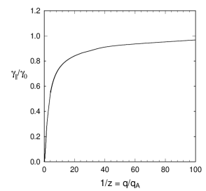
FIG. 3.: Scaling function for the line width of the spin fluctuations parallel to the easy axis of magnetization, $\gamma_{\parallel}(x,z)$, as a function of $q/q_{{}_{A}}$ at the critical temperature $x=0$ ($T=T_{c}$).

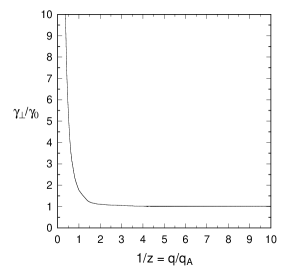
FIG. 4.: Scaling function for the line width of the spin fluctuations perpendicular to the easy axis of magnetization $\gamma_{\perp}(x,z)$ as a function of $q/q_{{}_{A}}$ at the critical temperature $x=0$ ($T=T_{c}$).

The physical content of the two parameter scaling surfaces is illustrated best by considering cuts for fixed $q_{{}_{A}}$ and various temperatures, since for a given material, $q_{{}_{A}}$ is fixed and the parametrisation by $\varphi$ corresponds to a parametrisation in terms of the reduced temperature $(T-T_{c})/T_{c}$. In Figs. 5-6 the scaling functions versus $x=1/q\xi$ are displayed for different values of $\varphi=\arctan(q_{{}_{A}}\xi)=N\pi/20$ with $N=0,1,...,9$. For $\varphi=0$, corresponding to vanishing uniaxial anisotropy $q_{{}_{A}}$, the scaling functions coincide with the Resibois-Piette scaling function [21]. If the strength of the uniaxial anisotropy $q_{{}_{A}}$ is finite, the curves for the scaling functions approach the Resibois-Piette scaling function for small values of the scaling variable $x$ and deviate therefrom with increasing $x$. At fixed scaling variable $x$ and with increasing temperature (increasing $\varphi$) the value of the scaling function for the spin fluctuations along the easy axis of magnetization is lowered with respect to the Resibois-Piette function, whereas it is increased for the scaling function of the spin fluctuations in the basal plane.

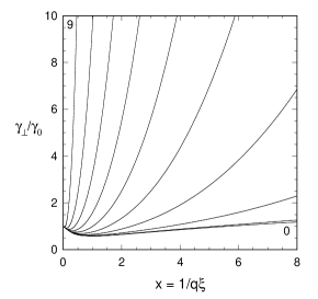
FIG. 5.: Scaling function for the linewidth of the spin fluctuations perpendicular to the easy axis of magnetization $\gamma_{\perp}$ as function of $x=1/q\xi$ for various angles $\varphi=N\pi/20$, with $N=0,\ldots,9$.

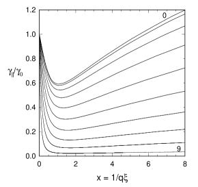
FIG. 6.: Scaling function for the linewidth of the spin fluctuations parallel to the easy axis of magnetization $\gamma_{\parallel}$ as function of $x=1/q\xi$ for various angles $\varphi=N\pi/20$, mit $N=0,\ldots,9$.

b Dipolar limit:

As summarized in Table III the mode coupling equations in the pure dipolar limit can be solved analytically in the dipolar (D) and isotropic (I) critical (C) and hydrodynamic (H) limiting regions. These are defined by DC: $y\gg 1$, $x\ll 1$; IC: $y\ll 1$, $x\ll 1$; DH: $y\gg x$, $x\gg 1$; IH: $y\ll x$, $x\gg 1$.

Concerning the critical dynamical exponent one finds for the longitudinal line width a crossover from $z={5/2}$ in the isotropic critical region to $z=0$ in the dipolar critical region, whereas for the transverse line width the crossover is from $z={5/2}$ to $z=2$. The precise position of this crossover can only be determined numerically.

A plot of the transverse and longitudinal scaling functions $\gamma^{T}(x,y)$ and $\gamma^{L}(x,y)$ can be found in Ref. [5]. For the dipolar crossover precisely at the Curie point the crossover from the isotropic Heisenberg to dipolar critical dynamics in the transverse line width occurs at a wave number, which is almost one order of magnitude smaller than the static crossover wave vector $q_{{}_{D}}$. The crossover of the longitudinal width, from $z=2.5$ to $z=0$, is more pronounced and occurs in the intermediate vicinity of $q_{{}_{D}}$. The reason for the different location of the dynamic crossover is mainly due to the fact that it is primarily the longitudinal static susceptibility which shows a crossover due to the dipolar interaction. Since the change in the static critical exponents is numerically small the transverse static susceptibility is nearly the same as for ferromagnets without dipolar interaction. Hence the crossover in the transverse width is purely a dynamical crossover, whereas the crossover of the longitudinal width being proportional to the inverse static longitudinal susceptibility is enhanced by the static crossover.

c General case:

For nonvanishing dipolar interaction and uniaxial anisotropy the mode coupling equations for the scaling functions of the spin fluctuations $s_{\alpha}({\bf q})$ are given by

$$\gamma_{\alpha}(\nu;{\bf R}) = \int_{0}^{\infty}d\rho\,\rho^{2}\int_{0}^{\pi}d\eta\sin\eta\int_{0}^{2\pi}d\sigma$$ (147)

$$\times {\hat{K}}^{\beta\gamma}_{\alpha}({\rho},{\hat{\bf q}};{\bf R})\,\frac{\hat{\chi}_{\beta}(\mathchoice{{\hbox{\boldmath$\displaystyle\rho$}}}{{\hbox{\boldmath$\textstyle\rho$}}}{{\hbox{\boldmath$\scriptstyle\rho$}}}{{\hbox{\boldmath$\scriptscriptstyle\rho$}}};{\bf R})\,\hat{\chi}_{\gamma}(\mathchoice{{\hbox{\boldmath$\displaystyle\rho$}}}{{\hbox{\boldmath$\textstyle\rho$}}}{{\hbox{\boldmath$\scriptstyle\rho$}}}{{\hbox{\boldmath$\scriptscriptstyle\rho$}}}_{-};{\bf R})}{\hat{\chi}_{\alpha}({\hat{\bf q}};{\bf R})}$$ (148)

$$\times \frac{1}{\rho^{\frac{5}{2}}\gamma_{\beta}(\eta;\frac{R}{\rho},\varphi,\theta)+\rho_{-}^{\frac{5}{2}}\gamma_{\gamma}(\eta_{-};\frac{R}{\rho_{-}},\varphi,\theta)},$$ (149)

where we have introduced polar coordinates

$${\bf R} = \left(\begin{array}[]{c}x\\ y\\ z\\ \end{array}\right)\,=\,\left(\begin{array}[]{c}R\,\cos\varphi\,\sin\theta\\ R\,\sin\varphi\,\sin\theta\\ R\,\cos\theta\\ \end{array}\right),$$ (156)

with

$$R \in [0;\infty[\qquad\varphi\,\in\,[0;\frac{\pi}{2}]\qquad\theta\,\in\,[0;\frac{\pi}{2}].$$ (157)

The mode coupling equations can be solved analytically only in some limiting cases. The results for these limiting cases are given table IV. In all other cases one has to solve the mode coupling equations numerically. For this it is best to write the scaling variables in spherical coordinates. The results for the three scaling functions are plotted in Figs. 7–9. In these figures we have plotted a table for each of the scaling functions, where in each element of the table the scaling function is shown as a function of the radial scaling variable $R$ for a set of angles of the wave vector with respect to the $z$-axis. The three colums (from left to right) correspond to the angles $\varphi=\pi/5$, $2\pi/5$ and $\pi/2$ and the rows (from top to bottom) correspond to $\theta=\pi/5$, $2\pi/5$ and $\pi/2$. Note that $\tan\varphi=q_{{}_{D}}\xi$ and $\tan\theta=\sqrt{\xi^{-2}+q_{{}_{D}}^{2}}/q_{{}_{A}}$.

The continuous crossover from isotropic to uniaxial or dipolar behavior can then be easily read off from Figs. 7–9.

• For $\varphi\rightarrow 0$ and $\theta\rightarrow\pi/2$ all three scaling functions become identical to the Resibois-Piette scaling function for the isotropic Heisenberg ferromagnet.

• In the uniaxial limit $\varphi\rightarrow 0$ (corresponding to $q_{{}_{D}}\rightarrow 0$) the first two scaling functions become identical.

• Variation of the anisotropy strength $q_{{}_{A}}$ in the weak dipolar limit ($q_{{}_{D}}\xi\ll 1$) (i.e., increasing $\theta$ from $0$ to $\pi/2$ for small values of $\varphi$) gives the transition from the Resibois-Piette function to the uniaxial limit discussed above. $\gamma_{1}$ and $\gamma_{2}$ become identical to the scaling function for the uncritical transverse modes whereas $\gamma_{3}$ becomes the scaling function for the fluctuations along the easy axis.

• For small uniaxial anisotropy ($q_{{}_{A}}\ll\sqrt{\xi^{-2}+q_{{}_{D}}^{2}}$ or equivalently $\theta$ close to $\pi/2$) one recovers the dipolar limit where $\gamma_{1}$ and $\gamma_{3}$ reduce to the two equivalent transverse modes, and $\gamma_{2}$ becomes the uncritical longitudinal mode.

• Upon going along the diagonal from top-left to bottom-right in Figs. 7–9 one crosses over from the uniaxial to the dipolar limit and $\gamma_{1}$ and $\gamma_{3}$ become more and more similar. The scaling function $\gamma_{2}$ makes a continuous crossover from the scaling function for the mode parallel to the easy axis (critical mode) in the uniaxial case to the scaling function of the longitudinal mode (uncritical mode) in the dipolar limit.

• The first mode $\gamma_{1}$ does not show any dependence on the orientation $\nu$ of the wave vector with respect to the $z$-axis. The reason is that this mode is by construction always perpendicular to both the $z$-axis and the wave vector ${\bf q}$ and hence idependent from the angle between these two axes.

• The second and third mode show no $\nu$-dependence neither in the dipolar nor in the uniaxial limit. The dependence on $\nu$ is strongest close to $\theta\approx\pi/4$ and $\varphi\approx\pi/4$. It is most pronounced for the third mode. This is due to the strong $\nu$-dependence of this mode in the hydrodynamic limit (see table IV). Whereas the scaling behavior of $\gamma_{1}$ and $\gamma_{2}$ does not depend on the orientation of the wave vector with respect to the $z$-axis in this limit.

• The effective dynamic exponents $z_{\rm eff}$ become zero for all three modes in the case $q_{{}_{D}}\neq 0$, except for $\gamma_{3}$ in the case $\nu=\pi/2$.

FIG. 7.: Scaling function $\gamma_{1}$ as a function of $R$ for various angles $\theta$ and $\varphi$. Each graph for fixed $\theta$ and $\varphi$ contains a set of curves parametrized by the angle $\nu$ of the wave vector with respect to the $z$-axis: $\nu=N\pi/8$ with $N=0,\cdots,4$.

FIG. 8.: Scaling function $\gamma_{2}$ as a function of $R$ for various angles $\theta$ and $\varphi$. Each graph for fixed $\theta$ and $\varphi$ contains a set of curves parametrized by the angle $\nu$ of the wave vector with respect to the $z$-axis: $\nu=N\pi/8$ with $N=0,\cdots,4$.

FIG. 9.: Scaling function $\gamma_{3}$ as a function of $R$ for various angles $\theta$ and $\varphi$. Each graph for fixed $\theta$ and $\varphi$ contains a set of curves parametrized by the angle $\nu$ of the wave vector with respect to the $z$-axis: $\nu=N\pi/8$ with $N=0,\cdots,4$.

d Gd – no magnetocrystalline anisotropy:

As we have already mentioned in the introduction Gd is a very interesting rare earth matrerial because it is an S-state ion with a large localized magnetic moment. Because of this it should have a very small magnetocrystalline anisotropy and be a much better model system for an isotropic Heisenberg ferromagnet than materials like Fe, EuO or EuS. Contrary to this expectation, however, experimental observations teach us that Gd has an easy axis which coincides with the hexagonal axis of its hcp structure. In the following section we will identify the dipole–dipole interaction in conjunction with the lattice structure as the source of this easy axis anisotropy. Then we can explicitely calculate the ratio of the two crossover wave vectors,

$$q_{{}_{D}}/q_{{}_{A}}=7.8738\,,$$ (158)

and thus reduce the number of material parameters by one. This allows us to present our theoretical results for the line widths of the correlation functions in the same way as for the two limiting cases of the cubic dipolar and purely uniaxial systems.

In Figures 10–12 we compare the scaling functions for the line widths of the three modes $\gamma_{1}$, $\gamma_{2}$ and $\gamma_{3}$ for the hcp dipolar model with the corresponding results for the cubic dipolar model. Since the dipolar interaction is the dominant anisotropy the deviations of the results for the hcp from the cubic model are small. For $\gamma_{1}$ and $\gamma_{3}$ we find that the relaxation times of the hcp system are reduced as compared to the cubic model. This seems plausible since – as discussed in section III – the induced uniaxial anisotropy supresses some of the critical fluctuations. This has to be contrasted with the behavior of $\gamma_{2}$, where the corresponding longitudinal mode in the cubic dipolar system is alread an uncritical mode. We find that the result for $\gamma_{2}$ is almost identical to the longitudinal scaling function of the cubic dipolar system.

FIG. 10.: Comparison of the scaling function $\gamma_{1}$ at $\nu=0$ of the hcp dipolar model (solid lines) with the transverse scaling function $\gamma_{T}$ (dashed lines) of the cubic dipolar model. The scaling functions are given as a function of $x=1/q\xi$ for various values of $\varphi=N\pi/20$ with $N=0,...,9$.

FIG. 11.: Comparison of the scaling function $\gamma_{2}$ at $\nu=0$ of the hcp dipolar model (solid lines) with the longitudinal scaling function $\gamma_{L}$ (dashed lines) of the cubic dipolar model. The scaling functions are given as a function of $x=1/q\xi$ for various values of $\varphi=N\pi/20$ with $N=0,...,9$.

FIG. 12.: Comparison of the scaling function $\gamma_{3}$ at $\nu=0$ of the hcp dipolar model (solid lines) with the transverse scaling function $\gamma_{T}$ (dashed lines) of the cubic dipolar model. The scaling functions are given as a function of $x=1/q\xi$ for various values of $\varphi=N\pi/20$ with $N=0,...,9$.

The case $\nu=\pi/2$ is special since here the third mode in the hcp model becomes critical (see section III). As a consequence there is no supression of critical fluctuations and one does not expect that dynamics is slowed down with respect to the cubic case. Indeed, as can be inferred from Fig. 13, the mode becomes even faster than in the cubic case.

The dependence on the relative orientation of the $c$-axis and the wave vector is not very pronounced. There is actually no $\nu$-dependence for $\gamma_{1}$ since this mode is by construction always perpendicular to the $c$-axis. In Figs. 14-15 we try to visualize the $\nu$-dependence of $\gamma_{2}$ and $\gamma_{3}$ at a set of parameters $q_{{}_{D}}\xi=1.0$ and $q_{{}_{A}}\xi=1.0$. These parameters do not correspond to Gd, because as we have already seen in Figs. 7-9, the angle dependence is largest when $q_{{}_{A}}$ and $q_{{}_{D}}$ are comparable; hence it is quite small for the hcp dipolar system Gd.

FIG. 13.: Comparison of the scaling function $\gamma_{3}$ at $\nu=\pi/2$ of the hcp dipolar model (solid lines) with the transverse scaling function $\gamma_{T}$ (dashed lines) of the cubic dipolar model. The scaling functions are given as a function of $x=1/q\xi$ for various values of $\varphi=N\pi/20$ with $N=0,...,9$.

FIG. 14.: Scaling function $\gamma_{2}$ for the hcp dipolar model as a function of $x=1/q\xi$ for fixed values $q_{{}_{D}}\xi=1.0$ and $q_{{}_{A}}\xi=1.0$ and a series of angles $\nu=N\pi/8$ with $N=0,1,\cdots,4$ indicated in the graph.

FIG. 15.: Scaling function $\gamma_{3}$ for the hcp dipolar model as a function of $x=1/q\xi$ for fixed values $q_{{}_{D}}\xi=1.0$ and $q_{{}_{A}}\xi=1.0$ and a series of angles $\nu=N\pi/8$ with $N=0,1,\cdots,4$ indicated in the graph.

Finally, let us discuss the behavior of the line width right at the critical temperature. Figs. 16–18 show the scaling functions of the three modes in the hcp system compared with the corresponding results for the cubic dipolar and the uniaxial system.

FIG. 16.: Scaling function $\gamma_{1}$ at the critical temperature as a function of $q/q_{{}_{D}}$ (solid line) compared with the corresponding transverse scaling function $\gamma_{{}_{T}}$ of the cubic dipolar system (dot-dashed line) and the hard axis scaling function $\gamma_{{}_{\perp}}$of the uniaxial system (dotted line). Note that in the uniaxial case the scaling function is plotted as a function of $q/q_{{}_{A}}$ but as a function of $q/q_{{}_{D}}$ for the dipolar cases.

FIG. 17.: Scaling function $\gamma_{2}$ at the critical temperature as a function of $q/q_{{}_{D}}$ for $\nu=0$ (solid line) and $\nu=\pi/2$ (dashed line) compared with the corresponding longitudinal scaling function $\gamma_{{}_{L}}$ of the cubic dipolar system (dot-dashed line) and the hard axis scaling function $\gamma_{{}_{\perp}}$ of the uniaxial system (dotted line). Note that in the uniaxial case the scaling function is plotted as a function of $q/q_{{}_{A}}$ but as a function of $q/q_{{}_{D}}$ for the dipolar cases.

Again, we find that for the parameter values of Gd there is little difference between the results for the cubic and the hcp dipolar system (but a huge difference to the results of a uniaxial model with no dipolar interaction). The most notable effect is that the crossover wave vector which marks the deviation from isotropic Heisenberg behavior (with a dynamic exponent $z=5/2$) is shifted to larger values for the first mode and to smaller values for the second and third mode. Then there is also a clearly visible dependence on the orientation of the wave vector with respect to the $c$–axis for the third mode.

FIG. 18.: Scaling function $\gamma_{3}$ at the critical temperature as a function of $q/q_{{}_{D}}$ for $\nu=0$ (solid line) and $\nu=\pi/2$ (dashed line) compared with the corresponding transverse scaling function $\gamma_{{}_{T}}$ of the cubic dipolar system (dot-dashed line) and the soft axis scaling function $\gamma_{{}_{\parallel}}$ of the uniaxial system (dotted line). Note that in the uniaxial case the scaling function is plotted as a function of $q/q_{{}_{A}}$ but as a function of $q/q_{{}_{D}}$ for the dipolar cases.

V Comparison with experimental data

The critical dynamics of Gd has been investigated experimentally almost exclusively by several nuclear, i.e., hyperfine interaction (HFI), methods. The application of nuclear techniques to study critical phenomena in magnets has recently been reviewed by Hohenemser et al. [25]. All of the hyperfine interaction methods are local probes which are related to a wave vector integral of the spin correlation functions. As such they offer a complement to neutron scattering. Dynamic studies, using hyperfine interaction probes, utilize the process of nuclear relaxation produced by time–dependent hyperfine interaction fields, which reflect fluctuations of the surrounding electronic magnetic moments.

The hyperfine interaction stems from the magnetic interaction of the electrons with the magnetic field produced by the nucleus. The hyperfine interaction of a nucleus with spin ${\bf I}$, $g$–factor $g_{N}$ and mass $m_{N}$ with one of the surrounding electrons with spin ${\bf S}$ and orbital momentum ${\bf L}$ can be written in the form [5]

$$H_{\rm hyp} = \frac{Ze_{0}^{2}g_{N}}{2m_{N}mc^{2}}\Biggl{[}\frac{1}{r^{3}}{\bf I}\cdot{\bf L}+\frac{8\pi}{3}\delta^{(3)}({\bf x})\,{\bf I}\cdot{\bf S}$$ (159)

$$-\frac{1}{r^{3}}{\bf I}\cdot{\bf S}+\frac{3({\bf I}\cdot{\bf x})({\bf S}\cdot{\bf x})}{r^{5}}\Biggr{]}\,.$$ (160)

The first term represents the interaction of the orbital momentum of the electron with the nuclear magnetic moment of the nucleus. The second term is the Fermi contact interaction and the last two terms represent the dipolar interaction. The Fermi contact interaction is finite only for electrons having a finite probability density at the nucleus, i.e. bound $s$-electrons or itinerant electrons. The Hamiltonian, Eq. (160), can also be used for the analysis of spin resonance experiments with muons ($\mu$SR). However, these do not have bound electrons and hence the Fermi contact term involves only conduction electrons and is of the same order of magnitude as the (residual) dipolar interaction [26].

A $\mu$SR measurement

As shown in appendix A the muon damping rate can be written as

$$\lambda_{\hat{z}}=\frac{\pi{\cal D}}{V^{2}}\int_{{\bf q}}\sum_{{\hat{\beta}}{\hat{\gamma}}}\left[G^{{\hat{x}}{\hat{\beta}}}_{\bf q}G^{{\hat{x}}{\hat{\gamma}}}_{-{\bf q}}+G^{{\hat{y}}{\hat{\beta}}}_{\bf q}G^{{\hat{y}}{\hat{\gamma}}}_{-{\bf q}}\right]\Phi^{{\hat{\beta}}{\hat{\gamma}}}({\bf q}),$$ (161)

where we have defined ${\cal D}=\gamma_{\mu}^{2}(\mu_{0}/4\pi)^{2}(g_{L}\mu_{B})^{2}$. The coupling of the muon spin and the spins of the magnet is described in terms of the coupling matrix $G^{{\hat{x}}{\hat{\beta}}}_{\bf q}$, which reflects the particular symmetry of the lattice sites occupied by the muons. Since the most dominant contribution to the damping rate comes from wave vectors close to the Brillouin zone center, the peculiar properties of the coupling tensor $G^{{\hat{x}}{\hat{\beta}}}_{\bf q}$ at small values of ${\bf q}$ will be important. The coupling tensor is determined by both the type of interaction between the muon spin and the spins of the magnet and the location of the muon in the lattice. As noted above the coupling contains dipolar interaction as well as a contribution from the Fermi contact field. Using a decomposition into four orthorhombic sublattices ($l=0,1,2,3$) the dipolar interaction can be written in the form [16],

$$D^{\alpha\beta}({\bf q}) = \sum_{l=0}^{3}\sum_{i}D^{\alpha\beta}({\bf r}_{i,l})\,e^{i{\bf q}\cdot{\bf r}_{i,l}},$$ (162)

where ${\bf r}_{i,l}={\bf i}+{\bf r}_{l}-{\bf r}_{0}$ denotes the position on site $i$ of sublattice $l$ with respect to the position of the muon ${\bf r}_{0}$. The lowest-order approximation in ${\bf q}$ of $D^{\alpha\beta}({\bf q})$ is given by (see appendix A)

$$D^{\alpha\beta}({\bf q}\to 0)=-4\pi\left[\frac{q_{\alpha}q_{\beta}}{q^{2}}-d_{\alpha}\right].$$ (163)

where we find for octahedral sites  [27]:

$$d_{x}=d_{y}=0.3485\quad\mbox{and}\quad d_{z}=0.3030,$$

and for tetrahedral sites

$$d_{x}=d_{y}=0.3118\quad\mbox{and}\quad d_{z}=0.3764.$$

Adding the isotropic contribution from the Fermi contact field one finds in the limit ${\bf q}\to 0$

$$G^{\alpha\beta}_{{\bf q}\to 0} = -4\pi\left[\frac{q_{\alpha}q_{\beta}}{q^{2}}-d_{\alpha}\right]+n_{\mu}H_{\mu}\delta_{\alpha\beta}$$ (164)

$$= -4\pi\left[\frac{q_{\alpha}q_{\beta}}{q^{2}}-p_{\alpha}\right],$$ (165)

with

$$p_{\alpha}=d_{\alpha}+\frac{n_{\mu}H_{\mu}}{4\pi}.$$ (166)

With the Fermi contact field $B_{\rm FC}=-6.98$ kG at $T=0$ K [26], one gets $n_{\mu}H_{\mu}/4\pi=-0.278$ [27], and consequently for octahedral sites

$$p_{x}=p_{y}=0.0705\quad\mbox{and}\quad p_{z}=0.0250,$$

and for tetrahedral sites

$$p_{x}=p_{y}=0.0338\quad\mbox{and}\quad p_{z}=0.0984.$$

Before comparing the theoretical result with experiments one has to find a transformation between the reference frames used in the theoretical analysis and the experimental setup, respectively. In Eq. 161 (i.e. in the experimental setup) one uses a reference frame $(\hat{x},\hat{y},\hat{z})$ which is fixed with respect to the initial polarization of the muon beam, which is choosen to be along the $\hat{z}$-axis. The reference frame used in the theoretical analysis, $(x,y,z)$ was chosen such that the $z$-axis coincides with the easy axis of magnetization. (see Fig. 19). The transformation rules are given by

$$\hat{x} = x,$$ (167)

$$\hat{y} = y\,\cos\alpha+z\,\sin\alpha,$$ (168)

$$\hat{z} = -y\,\sin\alpha+z\,\cos\alpha,$$ (169)

FIG. 19.: Reference frame $(\hat{x},\hat{y},\hat{z})$ for $\mu$SR measurements, which is rotated by $\alpha$ around the $x$–axis with respect to the reference frame $(x,y,z)$. Here $z$ is the direction of the easy axis of magnetization and ${\hat{z}}$ is the direction of the initial polarization of the muon beam.

Then the coupling tensor in the experimental reference frame reads

$$G^{\hat{x}\hat{x}}({\bf q}\to 0) = -4\pi\left[\frac{q_{x}^{2}}{q^{2}}-p_{x}\right],$$ (170)

$$G^{\hat{x}\hat{y}}({\bf q}\to 0) = -4\pi\left[\frac{q_{x}q_{y}}{q^{2}}\cos\alpha+\frac{q_{x}q_{z}}{q^{2}}\sin\alpha-p_{x}\right],$$ (171)

$$G^{\hat{x}\hat{z}}({\bf q}\to 0) = -4\pi\left[-\frac{q_{x}\ q_{y}}{q^{2}}\sin\alpha+\frac{q_{x}\ q_{z}}{q^{2}}\cos\alpha-p_{x}\right],$$ (172)

$$G^{\hat{y}\hat{x}}({\bf q}\to 0) = -4\pi\left[\frac{q_{x}q_{y}}{q^{2}}\cos\alpha+\frac{q_{x}q_{z}}{q^{2}}\sin\alpha-p_{y}\cos\alpha-p_{z}\sin\alpha\right],$$ (173)

$$G^{\hat{y}\hat{y}}({\bf q}\to 0) = -4\pi\Biggl{[}\frac{q_{y}^{2}}{q^{2}}\cos^{2}\alpha+2\frac{q_{y}q_{z}}{q^{2}}\sin\alpha\cos\alpha+\frac{q_{z}^{2}}{q^{2}}\sin^{2}\alpha-p_{y}\cos\alpha-p_{z}\sin\alpha\Biggr{]},$$ (174)

$$G^{\hat{y}\hat{z}}({\bf q}\to 0) = -4\pi\Biggl{[}\frac{q_{z}^{2}}{q^{2}}\sin\alpha\cos\alpha-\frac{q_{y}^{2}}{q^{2}}\cos\alpha\sin\alpha+\frac{q_{y}q_{z}}{q^{2}}(\cos^{2}\alpha-\sin^{2}\alpha)-p_{y}\cos\alpha-p_{z}\sin\alpha\Biggr{]}.$$ (175)

In the same way we find for the relation of the spin correlation functions in the reference frames defined with respect to the initial muon beam polarization and the easy axis of magnetization, respectively,

$$\Phi^{\hat{x}\hat{x}}({\bf q}) = \Phi^{xx}({\bf q}),$$ (176)

$$\Phi^{\hat{x}\hat{y}}({\bf q}) = \Phi^{\hat{y}\hat{x}}({\bf q})=\Phi^{xy}({\bf q})\cos\alpha+\Phi^{xz}({\bf q})\sin\alpha,$$ (177)

$$\Phi^{\hat{x}\hat{z}}({\bf q}) = \Phi^{\hat{x}\hat{z}}({\bf q})=\Phi^{xz}({\bf q})\cos\alpha-\Phi^{xy}({\bf q})\sin\alpha,$$ (178)

$$\Phi^{\hat{y}\hat{y}}({\bf q}) = \Phi^{yy}({\bf q})\cos^{2}\alpha+\Phi^{zz}({\bf q})\sin^{2}\alpha+2\Phi^{yz}({\bf q})\cos\alpha\sin\alpha,$$ (179)

$$\Phi^{\hat{y}\hat{z}}({\bf q}) = \Phi^{\hat{z}\hat{y}}({\bf q})=\Phi^{zz}({\bf q})\sin\alpha\cos\alpha-\Phi^{yy}({\bf q})\sin\alpha\cos\alpha+\Phi^{yz}({\bf q})(\cos^{2}\alpha-\sin^{2}\alpha),$$ (180)

$$\Phi^{\hat{z}\hat{z}}({\bf q}) = \Phi^{yy}({\bf q})\sin^{2}\alpha+\Phi^{zz}({\bf q})\cos^{2}\alpha-2\Phi^{yz}({\bf q})\cos\alpha\sin\alpha.$$ (181)

In section IV C we have calculated the spin correlation functions $\bar{\Phi}^{\alpha\alpha}({\bf q})$ in the eigenvector basis ${\bf e}_{\alpha}({\bf q})$. Upon using the transformation, Eq. 76, between cartesian spin components and the spin components in the eigenvector basis we find

$$\Phi^{\beta\gamma}({\bf q})=\sum_{\alpha}w_{\alpha\beta}({\bf q})w_{\alpha\gamma}({\bf q})\bar{\Phi}^{\alpha\alpha}({\bf q}).$$ (182)

With the Fluctuation-Dissipation-Theorem the spin correlation functions $\bar{\Phi}^{\alpha\beta}({\bf q})$ are given in terms of the statical susceptibility and the linewidth,

$$\bar{\Phi}^{\alpha\alpha}({\bf q}) = \frac{2k_{B}T}{\mu_{0}(g_{L}\mu_{B})^{2}}\frac{\chi_{\alpha}({\bf q})}{\Gamma^{\alpha}({\bf q})}$$ (183)

$$= \frac{2k_{B}T}{J\mu_{0}(g_{L}\mu_{B})^{2}Aq^{z+2}}\frac{1}{\hat{\lambda}_{\alpha}({\bf R})\,\gamma_{\alpha}(\nu;{\bf R})}.$$ (184)

The muon relaxation rate $\lambda_{z}$ depends on the material parameters $q_{{}_{A}}\xi_{0}$ and $q_{{}_{D}}\xi_{0}$ characterizing the strength of the uniaxial anisotropy and the dipolar interaction, respectively. If we assume that the uniaxial anisotropy in Gd is solely due to the combined effect of dipolar interaction and non cubic lattice structure, one can estimate the ratio of dipolar to uniaxial wave vector [16]

$$\frac{q_{{}_{D}}}{q_{{}_{A}}}=7.8738.$$ (185)

With this assumption the number of material parameters is reduced to one, $q_{{}_{D}}\xi_{0}$. In comparing our theory with $\mu$SR experiments at a polarization $\alpha=90^{o}$ we get the best fit to the data with $q_{{}_{D}}\xi_{0}=0.13$. This results in the following values for the uniaxial and dipolar wave vector

$$q_{{}_{A}}=0.0165/\xi_{0},\quad q_{{}_{D}}=0.13/\xi_{0}.$$ (186)

The corresponding crossover temperatures, $q_{A,D}\xi=1$, are given by

$$T_{A}=T_{c}+0.43\,{\rm K},\quad T_{D}=T_{c}+16.54\,{\rm K}.$$ (187)

These set of parameters suggest the following crossover scenario. For $T\gg T_{D}$ we expect critical behavior dominated by the (isotropic) Heisenberg fixed point. The relaxation rate shows power law behavior

$$\lambda\propto t^{-w},$$ (188)

with an exponent $w_{\rm I}\approx\nu(z-1)\approx 1$. For temperatures in the interval $T_{D}>T>T_{A}$ dipolar interaction becomes important. But, from our analysis of the uniaxial crossover in section IV C we have seen that the uniaxial crossovers in dynamics sets in at wave vectors much larger than expected from an analysis of the static quantities; i.e., the dynamic crossover in the longitudinal scaling function right at $T_{c}$ is located at $q_{\rm cross}\approx 10\times q_{{}_{A}}$. Therefore, even for $T>T_{A}$ we expect to observe effects from dipolar interaction as well as uniaxial anisotropy. Finally, for $T<T_{A}$ the critical dynamics is determined by the uniaxial dipolar fixed point. Then the static susceptibilities do no longer diverge for $q\rightarrow 0$ and $T\rightarrow T_{c}$ except when the wave vector ${\bf q}$ is perpendicular to the easy axis of magnetization. Since the relaxation rate $\lambda_{z}$ is given by an integral over the whole Brillouin zone, the relative weight of the critical axis along which the susceptibility diverges becomes vanishingly small. As a consequence the relaxation rate $\lambda_{z}$ no longer diverges for $T\rightarrow T_{c}$.

Since the interaction between the spin of the muon and the lattice spins is a combination of Fermi contact and dipolar interaction, the muon relaxation rate is a rather complicated function of the relaxation rates along the eigendirections. Therefore, the temperature dependence of the relaxation rate can no longer be described in terms of simple power laws but shows a more complicated functional dependence. In Figs. 20 and 21 we show a comparison between the theoretical and experimental results for two different initial polarizations.

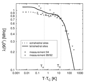
FIG. 20.: Experimental and theoretical results of the relaxation rate $\lambda$ for tetrahedral and octahedral muon sites with $\alpha=90^{o}$.

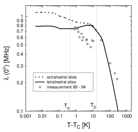
FIG. 21.: Experimental and theoretical results of the relaxation rate $\lambda$ for tetrahedral and octahedral muon sites with $\alpha=0^{o}$.

In Fig. 20 the initial polarization is inclined by an angle $\alpha=90^{o}$ with respect to the easy axis of magnetization. The solid line and dashed line are the theoretical result for the muon relaxation rate if the muons penetrating the sample are located at tetrahedral and octahedral interstitial sites, respectively. The comparison between theory and experiment favors tetrahedral sites. This is confirmed by $\mu$SR experiments with the initial polarization along the easy axis of magnetization (see Fig. 21). The ratio $\lambda_{z}(90^{o})/\lambda_{z}(0^{o})$ for $T\rightarrow T_{c}$ becomes $1.2$ and $0.7$ for octahedral and tetrahedral sites, respectively. The experiment is closer to the latter value.

B PAC and MS measurements

Here we consider those hyperfine interaction probes (ME, PAC, NMR), where the Fermi contact term gives the dominant contribution to the hyperfine field at the nucleus. Then the corresponding interaction Hamiltonian reduces to

$$H(t)=A_{\rm Fermi}\,{\bf I}\cdot{\bf S}(t)$$ (189)

where ${\bf I}$ denotes the nuclear and ${\bf S}$ the electronic spin. In hyperfine interaction experiments one observes the nuclear relaxation rate due to the surrounding fluctuating electronic magnetic moments. The standard experiments are performed in the motional narrowing regime, where the nuclear relaxation rate $\tau_{R}^{-1}$ is directly proportional to the (averaged) spin autocorrelation time $\tau_{c}$

$$\tau_{c}=\frac{1}{2}\int_{-\infty}^{\infty}dt\frac{1}{3}\sum_{\alpha}\Phi^{\alpha\alpha}({\bf x}=0,t),$$ (190)

where the spin autocorrelation function is given by

$$\Phi^{\alpha\alpha}({\bf R},t)=\frac{1}{2}\Bigl{\langle}\{S^{\alpha}({\bf x},t),S^{\alpha}({\bf 0},0)\}\Bigr{\rangle}.$$ (191)

Hence the above hyperfine interaction methods provide an integral property of the spin-spin correlation function. Upon using the fluctuation dissipation theorem (FDT) we get

$$\tau_{c}=\frac{k_{B}\,T}{V_{q}}\int_{\rm BZ}d^{3}{\bf q}\,\frac{1}{3}\sum_{\alpha}\frac{\chi_{\alpha}({\bf q};\xi,q_{{}_{D}},q_{{}_{A}})}{\Gamma_{\alpha}({\bf q};\xi,q_{{}_{D}},q_{{}_{A}})}.$$ (192)

The ${\bf q}$-integration extends over the Brillouin zone (BZ), the volume of which is $V_{q}$.

Important information about the behavior of the auto-correlation time can be gained from a scaling analysis. Upon using the static and dynamic scaling laws Eq. (192) can be written as

$$\tau_{c}\propto 4\pi\int dqq^{-z}{1\over 3}\sum_{\alpha}\frac{{\hat{\chi}}_{\alpha}\left({\hat{\bf q}};q\xi,q/q_{{}_{D}},q/q_{{}_{A}}\right)}{\gamma_{\alpha}\left({\hat{\bf q}};q\xi,q/q_{{}_{D}},q/q_{{}_{A}}\right)}\,,$$ (193)

where we have neglected the Fisher exponent $\eta$. If there were no dipolar interaction and no uniaxial anisotropy, one could extract the temperature dependence from the integral in Eq. (193) with the result $\tau_{c}\propto\xi^{z-1}$. This expression can be used to define an effective dynamical exponent $z_{\rm eff}(\tau)$, which depends on the correlation length by

$$\tau_{c}\propto\xi^{z_{\rm eff}-1}\propto\left({T-T_{c}\over T_{c}}\right)^{-w_{\rm eff}}\,.$$ (194)

with $w_{\rm eff}=\nu(z_{\rm eff}-1)$.

If dipolar interaction and uniaxial anisotropy are absent, one would expect to observe a critical exponent for the relaxation rate $w\approx 0.70\times(5/2-1)\approx 1.0$. Dipolar interaction is known to be a relevant perturbation with respect to the Heisenberg fixed point; it leads to asymptotic static critical exponents which are only slightly different from the corresponding Heisenberg values, but since dipolar interaction implies a non-conserved order parameter the asymptotic dynamic exponent becomes $z_{\rm D}\approx 2$. Hence dipolar interaction would induce a crossover from $w_{\rm I}\approx 1.0$ to $w_{\rm D}\approx 0.7$. Uniaxial interaction is also known to be a relevant perturbation with respect to the Heisenberg fixed point. Again, the static critical exponents are not changed very much, e.g. one finds $\nu_{\rm I}=0.63$, but the dynamic exponent becomes $z_{\rm I}\approx 4$ if the order parameter is conserved ($z_{\rm I}\approx 2$ otherwise). The corresponding exponent for the hyperfine relaxation rate would turn out to be $w_{\rm I}\approx 1.89$ and $w_{\rm I}\approx 0.63$ for conserved and non-conserved order parameter, respectively. According to these scaling arguments it is hard to think of any dynamic universality class which could lead to an effective exponent $w_{\rm eff}$ smaller than about $0.6$. Actually, however Mössbauer studies and PAC measurements on Gd show distinctly anomalous low values $w\approx 0.5$, which can not be explained by either of the above scenarios. This experimental puzzle can be resolved if one considers the combined effect of dipolar interaction and uniaxial anisotropy. As we have seen in our analysis of the static critical behavior of uniaxial dipolar ferromagnets, all the eigenvalues of the susceptibility matrix remain finite upon approaching the critical temperature except when the wave vector of the spin fluctuations is perpendicular to the easy axis of magnetization. Since this is only a region of measure zero in the Brillouin zone one actually expects that the relaxation rate Eq. (192) does no longer diverge upon approaching $T_{c}$, i.e., $w_{\rm UD}=0$. For a quantitative comparison with the experiment [28, 29, 30] we rewrite the auto correlation time in scaling form

$$\tau_{c} = \frac{2\pi\,k_{B}\,T}{J\,V\,A}\left(\xi^{-2}\!+\!q_{{}_{D}}^{2}\!+\!q_{{}_{A}}^{2}\right)^{-3/4}\int_{R_{0}}^{\infty}dR\,R^{1/2}$$ (196)

$$\times\int_{0}^{\pi}d\nu\sin\nu\,\frac{1}{3}\sum_{\alpha}\frac{1}{\hat{\lambda}_{\alpha}(\nu;{\bf R})\,\gamma^{\alpha}(\nu;{\bf R})},$$

where we have introduced polar coordinates. The lower cutoff is given by

$$R_{0}=\frac{1}{q_{{}_{\rm BZ}}}\sqrt{\xi^{-2}+q_{{}_{D}}^{2}+q_{{}_{A}}^{2}},$$ (197)

where $q_{\rm BZ}$ is the boundary of the Brillouin zone. In the critical region it can be disregarded and replaced by $R_{0}=0$, since $q_{{}_{\rm BZ}}\gg q_{{}_{D}},\,q_{{}_{A}}$ and the integrand in Eq. (196) is proportional to $\sqrt{R}$ for small $R$. For very small $\xi$ (outside the critical region) the cutoff reduces the autocorrelation time with respect to the critical value. One should note, that the dominant wave vectors contributing to the relaxation time $\tau_{c}$ in Eq. (196) are close to the zone center [27].

Let us now compare with hyperfine experiments on Gd mentioned above [29, 28, 30]. The autocorrelation time $\tau_{c}$ is shown in Figs. 22 and 23 for PAC experiments and Mössbauer spectroscopy, respectively. Both set of data are in good agreement with the results from mode coupling theory for $T-T_{c}<10K$. Note that besides the overall frequency scale there is no fit-parameter, since we have used the same set of values for the dipolar and uniaxial wave vector as for our comparison with $\mu$SR experiments. At higher temperatures the PAC data are above and the Mössbauer data below the theoretical prediction.

FIG. 22.: Experimental and theoretical results of the autocorrelation time $\tau_{c}$ for PAC experiments.

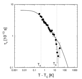
FIG. 23.: Experimental and theoretical results of the autocorrelation time $\tau_{c}$ for Mössbauer spectroscopy experiments.

The dipolar and uniaxial crossover temperatures indicated in the figures show that all the data are within the crossover regime between isotropic dipolar and uniaxial dipolar critical behavior. This explains the anomalous low value for the effective exponent $w\approx 0.5$. This result clearly shows for the first time that the universality class for the critical behavior of Gd is the uniaxial dipolar ferromagnet.

VI Summary and Conclusions

We have studied the critical dynamics of three-dimensional ferromagnets with uniaxial anisotropy taking into account exchange and dipole-dipole interaction. This analysis was mainly motivated by the puzzling experimental situation for the rare earth material Gd. Due to the fact that it is an S-state ion one would expect that it should have a vanishing magnetocrystalline anisotropy and therefore be an almost ideal model system for an isotropic Heisenberg ferromagnet (model J). But, the actual experimental observation shows large deviations from the expected behavior. As explained in detail in the main text, the way out of this puzzle is to realize that there is always a dipolar interaction between the magnetic moments in the material which in conjunction with the crystalline anisotropy can lead to anisotropy in the magnetic properties of the system.

The dipolar interaction and uniaxial anisotropy introduce two length scales, the dipolar wave vector $q_{{}_{D}}$ and the wave vector $q_{{}_{A}}$ measuring the uniaxial anisotropy. Note that there are two sources for the uniaxial anisotropy: magnetocrystalline (non S-state character of the magnetic ions) and dipolar. For Gd there is only the latter and hence $q_{{}_{D}}$ and $q_{{}_{A}}$ are not really independent but their ratio is fixed, $q_{{}_{D}}/q_{{}_{A}}=7.87$. Both length scales then have a common source, the dipole-dipole interaction.

The presence of these length scales leads to a quite complicated crossover scenario already for the static spin-spin correlation function. The essence of the physics, however, can already be seen within an Ornstein-Zernike approximation. Without uniaxial anisotropy two out of the three eigenmodes of the correlation function are critical, whereas the third correlation function starts to saturate once the wave vector becomes smaller than the dipolar wave vector $q_{{}_{D}}$. It is quite remarkable that due to the combined effect of dipolar and uniaxial anisotropy all eigenvalues of the susceptibilty matrix remain finite in the long wave length limit and upon approaching the critical temperature. Only if the angle $\nu$ between the easy axis of magnetization and the wave vector is $\nu=90^{o}$ the third eigenvalue (corresponding to the transverse mode when uniaxiality is neglected) becomes critical.

We have used mode coupling theory to derive a set of integral equations for the time-dependent spin-spin correlation functions. Using the Lorentzian approximation we have solved these equations numerically and determined the complete dynamic crossover scenario. Spezializing to Gd with a relatively weak uniaxial anisotropy (induced by the dipolar interaction) we find that the scaling functions for the line widths show a behavior which is similar to what is found for cubic dipolar systems (with no uniaxial anisotropy). The deviations become largest as the critical temperature is approached.

In the final section we have compared our results with $\mu$SR, PAC and Mössbauer experiments and find quantitative agreement with our theory. This explains the anomously low values of the critical exponents found in these experiments as a combined effect of lattice structure and dipolar interaction. From the quantitative agreement between theory and experiment the following conclusions can be drawn:

(i) The universality class of Gd is the uniaxial dipolar ferromagnet.

(ii) The dominant factor for the uniaxial anisotropy in Gd is solely the dipolar interaction.

(iii) The theory even allows us to predict that muons in Gd are located at tetrahedral interstitial sites close to $T_{c}$. We expect that the analysis presented in this paper will be valuable for interpreting dynamic measurements on the non-cubic magnetic system.

A Zero-field $\mu$SR depolarization rate and spin correlation functions

It can be shown [31] that the muon damping rate in longitudinal geometry is related to the spin-spin correlation function of the host material by a sum over all lattice sites

$$\lambda_{z} = \frac{\pi{\cal D}}{V^{2}}\sum_{i_{1}i_{2}}\sum_{\beta\gamma}\Biggl{[}G^{x\beta}({\bf r}_{i_{1}})G^{x\gamma}({\bf r}_{i_{2}})\Phi_{i_{1}i_{2}}^{\beta\gamma}$$ (A2)

$$\quad+G^{y\beta}({\bf r}_{i_{1}})G^{y\gamma}({\bf r}_{i_{2}})\Phi_{i_{1}i_{2}}^{\beta\gamma}\Biggr{]}$$

where ${\bf r}_{i}$ is the vector pointing from the interstitial position of the muon to the lattice site $i$. Here we have defined ${\cal D}=(\mu_{0}/4\pi)^{2}\gamma_{\mu}^{2}(g_{L}\mu_{B})^{2}$. Note that the sum is weighted by the coupling tensor $G^{\alpha\beta}({\bf r}_{i})$ of the muon and the spins of the magnet,

$$G^{\alpha\beta}({\bf r}_{i})=D^{\alpha\beta}({\bf r}_{i})+n_{\mu}\,H({\bf r}_{i})\delta_{\alpha\beta},$$ (A3)

with the dipolar contribution

$$D^{\alpha\beta}({\bf r}_{i})=v_{a}\left[\frac{3r_{i}^{\alpha}r_{i}^{\beta}}{r_{i}^{5}}-\frac{\delta_{\alpha\beta}}{r_{i}^{3}}\right]$$ (A4)

and the Fermi contact contribution $H_{{\bf r}_{i}}$, which equals $H$ for nearest-neighbor atoms and zero otherwise. The number of nearest neighbors equals $n_{\mu}$. $\Phi_{ij}^{\alpha\beta}$ is the symmetrized spin-spin correlation function between spins at sites $i_{1}$ and $i_{2}$ and zero frequency.

$$\Phi_{i_{1}i_{2}}^{\beta\gamma}\!=\!\frac{1}{2}[\langle S_{i_{1}}^{\beta}(\omega=0)S_{i_{2}}^{\gamma}\rangle\!+\!\langle S_{i_{2}}^{\gamma}(\omega=0)S_{i_{1}}^{\beta}(\omega=0)\rangle]$$ (A5)

Now we are going to rewrite Eq. (A2) in Fourier space. This leads to the evaluation of dipole sums

$$D^{\alpha\beta}({\bf q)}=\sum_{i}D^{\alpha\beta}({\bf r}_{i})e^{i{\bf q}\cdot{\bf r}_{i}}.$$ (A6)

How one deals with such dipole sums for cubic lattices has been described in Ref. [32]. Here we have to calculate the dipole sum for lattices with a hcp structure. This is most conveniently done by decomposing the lattice into four orthorombic sublattices such that each site is in exactly one sublattice [16]. The basis lattice vectors of the sublattices in terms of the basis vectors of the hcp lattice are given by

$${\bf a}_{1}={\bf a},\quad{\bf a}_{2}=2{\bf b}+{\bf a},\quad\text{and}\quad{\bf a}_{3}={\bf c}.$$ (A7)

The volume of an orthorhombic unit cell $v_{\rm ortho}$ is four times the volume $v_{hcp}$ per atom in gadolinium,

$$v_{\mathrm{hcp}}=\frac{1}{4}v_{\mathrm{ortho}}.$$ (A8)

A convenient choice of the origins of the four sublattices in terms of the basis vectors ${\bf a}_{1}$, ${\bf a}_{2}$ and ${\bf a}_{3}$ is

$${\bf R}_{0} = 0$$ (A9)

$${\bf R}_{1} = \frac{1}{2}{\bf a}_{1}+\frac{1}{2}{\bf a}_{2}$$ (A10)

$${\bf R}_{2} = \frac{1}{3}{\bf a}_{2}+\frac{1}{2}{\bf a}_{3}$$ (A11)

$${\bf R}_{3} = \frac{1}{2}{\bf a}_{1}+\frac{5}{6}{\bf a}_{2}+\frac{1}{2}{\bf a}_{3}.$$ (A12)

The muon can either be located at a tetrahedral site

$${\bf r}_{0}=\frac{3}{8}{\bf a}_{3},$$ (A13)

or a octahedral site

$${\bf r}_{0}=\frac{1}{2}{\bf a}_{1}+\frac{1}{6}{\bf a}_{2}+\frac{1}{4}{\bf a}_{3}.$$ (A14)

Putting things togehter we find

$$\lambda_{z}=\frac{\pi{\cal D}}{V^{2}}\sum_{l_{1}l_{2}}\sum_{i_{1}i_{2}}\sum_{\beta\gamma}\left[G^{x\beta}({\bf r}_{0}\!+\!{\bf i}_{1}\!+\!{\bf R}_{l_{1}})G^{x\gamma}({\bf r}_{0}\!+\!{\bf i}_{2}\!+\!{\bf R}_{l_{2}})+G^{y\beta}({\bf r}_{0}\!+\!{\bf i}_{1}\!+\!{\bf R}_{l_{1}})G^{y\gamma}({\bf r}_{0}\!+\!{\bf i}_{2}\!+\!{\bf R}_{l_{2}})\right]\Phi^{\beta\gamma}_{{\bf i}_{1}+{\bf R}_{l_{1}},{\bf i}_{2}+{\bf R}_{l_{2}}}$$ (15)

Introducing Fourier transformed spin variables for each of the sublattices

$$S^{\alpha}({\bf r}_{0}+{\bf i}+{\bf R}_{l})=\frac{1}{N}\sum_{{\bf q}}\exp[i{\bf q}\cdot({\bf r}_{0}+{\bf i}+{\bf R}_{l})]\,S^{\alpha}_{l}({\bf q})$$ (16)

where ${\bf R}_{l}$ are the lattice vectors of the $l$-th sublattice, one gets

$$\lambda_{z}=\pi\gamma_{\mu}^{2}\left(\frac{\mu_{0}}{4\pi}\right)^{2}\frac{(g_{L}\mu_{B})^{2}}{V^{2}}\sum_{{\bf q}}\sum_{\beta\gamma}\left[G^{x\beta}({\bf q})G^{x\gamma}(-{\bf q})+G^{y\beta}({\bf q})G^{y\gamma}(-{\bf q})\right]\Phi^{\beta\gamma}({\bf q}),$$ (17)

where the Fourier transform for the symmetrized spin-spin correlation function and the coupling tensor reads

$$G^{\alpha\beta}({\bf q}) = \sum_{l=0}^{3}\sum_{i}G^{\alpha\beta}({\bf r}_{0}+{\bf i}+{\bf R}_{l})\exp[i{\bf q}\cdot({\bf r}_{0}+{\bf i}+{\bf R}_{l})]$$ (18)

$$\Phi^{\beta\gamma}_{{\bf i}_{1}+{\bf R}_{l_{1}},{\bf i}_{2}+{\bf R}_{l_{2}}} = \frac{1}{N^{2}}\sum_{{\bf q}}\exp[i{\bf q}\cdot({\bf i}_{1}-{\bf i}_{2})]\exp[i{\bf q}\cdot({\bf R}_{l_{1}}-{\bf R}_{l_{2}})]\Phi^{\beta\gamma}({\bf q})$$ (19)

$$= \frac{1}{N^{2}}\sum_{{\bf q}}\exp[i{\bf q}\cdot(({\bf r}_{0}+{\bf R}_{l_{1}}+{\bf i}_{1})-({\bf r}_{0}+{\bf R}_{l_{2}}+{\bf i}_{2}))]\Phi^{\beta\gamma}({\bf q})$$ (20)

$$\Phi^{\beta\gamma}({\bf q}) = \frac{1}{2}\left[\langle S^{\beta}_{\bf q}(\omega=0)S^{\gamma}_{-{\bf q}}(\omega=0)\rangle+\langle S^{\gamma}_{-{\bf q}}(\omega=0)S^{\beta}_{\bf q}(\omega=0)\rangle\right]$$ (21)

The summation over ${\bf q}$ runs over the $N$ vectors in the first Brillouin zone. For sufficiently large $N$ the summation may be replaced by an integral

$$\lambda_{z}=\frac{\pi{\cal D}}{V}\int_{{\bf q}}\sum_{\beta\gamma}\left[G^{x\beta}_{\bf q}G^{x\gamma}_{-{\bf q}}+G^{y\beta}_{\bf q}G^{y\gamma}_{-{\bf q}}\right]\Phi^{\beta\gamma}({\bf q}).$$ (22)

In principle the damping rate $\lambda_{z}$ depends on the wave vector dependence of the coupling tensor and the symmetrized spin-spin correlation function over the whole Brillouin zone. It was shown, however, in Ref. [33] that in $\mu$SR measurements close to $T_{c}$ the dominant contribution to $\lambda$ comes from the vicinity of the Brillouin zone center. The coupling tensor $G^{\alpha\beta}({\bf q})$ can therefore be approximated by its limiting behavior near $q\to 0$.

Now we turn to the evaluation of the dipolar sums in the coupling tensor. The dipolar sums can be evaluated in Fourier space by the method of Ewald summation. The sum in Fourier space is divided in a sum over the direct lattice and a sum over the indirect lattice, so that both sums converge quickly.

With the decomposition into four orthorombic sublattices we get

$$D^{\alpha\beta}({\bf q}) = \sum_{l=0}^{3}\sum_{i}D^{\alpha\beta}({\bf r}_{i,l})\,\exp\left[i{\bf q}\cdot({\bf r}_{i,l})\right]$$ (23)

$$= \sum_{l=0}^{3}\sum_{i}D^{\alpha\beta}({\bf i}+{\bf R}_{l}-{\bf r}_{0})\,\exp\left[i{\bf q}\cdot({\bf i}+{\bf R}_{l}-{\bf r}_{0})\right]$$ (24)

$$= v_{{\rm hcp}}\sum_{l=0}^{3}\exp[i{\bf q}\cdot({\bf r}_{0}+{\bf R}_{l})]\left[\frac{\partial^{2}}{\partial x_{\alpha}\,\partial x_{\beta}}\left(\sum_{i}\frac{\exp(i{\bf q}\cdot{\bf i})}{|{\bf i}-{\bf x}|}\right)\right]_{{\bf x}={\bf r}_{0}-{\bf R}_{l}}.$$ (25)

The latter expression can be evaluated in the same way as for cubic lattices [32]. One finds [31]

$$D^{\alpha\beta}({\bf q}) = \frac{1}{4}\sum_{l=0}^{3}D_{l}^{\alpha\beta}({\bf q})=-4\pi\left[\frac{q_{\alpha}q_{\beta}}{q^{2}}-\frac{1}{4}\sum_{l=0}^{3}C_{l}^{\alpha\beta}({\bf q})\right]=-4\pi\left[\frac{q_{\alpha}q_{\beta}}{q^{2}}-C^{\alpha\beta}({\bf q})\right],$$ (26)

where

$$C_{l}^{\alpha\beta}({\bf q}) = 4\pi\frac{q_{\alpha}q_{\beta}}{q^{2}}\left[1-\exp\left(-\frac{q^{2}}{4\rho^{2}}\right)\right]-\frac{1}{4\rho^{2}}\sum_{{\bf K}\not=0}(K_{\alpha}+q_{\alpha})(K_{\beta}+q_{\beta})\varphi_{0}\left(\frac{({\bf q}+{\bf K})^{2}}{4\rho^{2}}\right)\exp[-i{\bf K}\cdot({\bf R}_{l}-{\bf r}_{0})]$$ (28)

$$+\frac{v\rho^{3}}{2\pi^{3/2}}\sum_{i}\Bigl{[}2\rho^{2}({\bf R}_{l}+{\bf i}-{\bf r}_{0})_{\alpha}({\bf R}_{l}+{\bf i}-{\bf r}_{0})_{\beta}\,\varphi_{3/2}(\rho^{2}r_{i}^{2})-\delta_{\alpha\beta}\,\varphi_{1/2}(\rho^{2}r_{i}^{2})\,\exp[i{\bf q}\cdot({\bf R}_{l}+{\bf i})-{\bf r}_{0}]\Bigr{]}.$$

To lowest order in $q$ this reduces to

$$D^{\alpha\beta}({\bf q}\to 0)=-4\pi\left[\frac{q_{\alpha}q_{\beta}}{q^{2}}-C^{\alpha\beta}({\bf q}=0)\right],$$ (29)

with

$$C^{\alpha\beta}({\bf q}=0)=\left(\begin{array}[]{ccc}0.3485&0&0\\ 0&0.3485&0\\ 0&0&0.3030\\ \end{array}\right)$$ (30)

for octahedral and

$$C^{\alpha\beta}({\bf q}=0)=\left(\begin{array}[]{ccc}0.3118&0&0\\ 0&0.3118&0\\ 0&0&0.3764\\ \end{array}\right)$$ (31)

for tetrahedral sites.

	$D^{xx}(=D^{yy})$	$D^{zz}$	$D^{xy}$	$D^{xz}(=D^{yz})$
$\beta_{1}^{\alpha\beta}$			0.44	0.53
$\beta_{2}^{\alpha}$	-0.16	-0.11
$\beta_{1}^{\alpha\alpha}-\beta_{3}^{\alpha}$	0.44	0.31
$\beta_{4}^{\alpha}$	4.12	4.32
$\beta_{z}$	-0.06

TABLE I.: Coefficients in the expansion of the dipolar tensor for a hcp lattice structure with $c=5.78\AA$, $a=3.62\AA$, and $c/a=1.59$, as appropriate for Gd bear $T_{c}$. Values are obtained from Ref. [16] upon multipying with the volume of the primitive cell $v_{a}$.

region	$\Gamma_{\perp}$	$\Gamma_{\parallel}$
UC	$q_{{}_{A}}^{{5/2}}$	$q_{{}_{A}}^{-{3/2}}q^{4}$
UH	$q_{{}_{A}}^{{5/2}}$	$q_{{}_{A}}^{-{3/2}}\,\xi^{-2}\,q^{2}$
IC	$q^{{5/2}}$	$q^{{5/2}}$
IH	$\xi^{-{1/2}}q^{2}$	$\xi^{-{1/2}}q^{2}$

C :	critical	U :	uniaxial
H :	hydrodynamic	I :	isotropic

TABLE II.: Analytic results for the asymptotic behavior of the transverse and longitudinal line widths for aniotropic ferromagnets with a uniaxial magneto-crystalline anisotropy, where the spins are coupled by short range exchange interaction only.

region	$\Gamma_{T}$	$\Gamma_{L}$
DC	$q_{{}_{D}}^{{1/2}}q^{2}$	$q_{{}_{D}}^{{5/2}}$
DH	$q_{{}_{D}}^{{1/2}}\,\xi^{-2}\,$	$q_{{}_{D}}^{{5/2}}$
IC	$q^{{5/2}}$	$q^{{5/2}}$
IH	$\xi^{-{1/2}}q^{2}$	$\xi^{-{1/2}}q^{2}$

C :	critical	D :	dipolar
H :	hydrodynamic	I :	isotropic

TABLE III.: Analytic results for the asymptotic behavior of the transverse and longitudinal linewidths for isotropic dipolar ferromagnets, where the spins are coupled by short-range exchange interaction and long-range dipolar interaction.

region	$\Gamma_{1}$	$\Gamma_{2}$	$\Gamma_{3}$
UDC $\nu\not=90^{o}$	$q_{{}_{A}}^{{5/2}}$	$q_{{}_{A}}^{{5/2}}$	$q_{{}_{A}}^{{5/2}}$
UDC $\nu=90^{o}$	$q_{{}_{A}}^{{5/2}}$	$q_{{}_{A}}^{{5/2}}$	$q_{{}_{A}}^{{1/2}}\,q^{2}$
DUC $\nu\not=90^{o}$	$q_{{}_{D}}^{{1/2}}\,q_{{}_{A}}^{2}$	$q_{{}_{D}}^{{5/2}}$	$q_{{}_{D}}^{{5/2}}$
DUC $\nu=90^{o}$	$q_{{}_{D}}^{{1/2}}\,q_{{}_{A}}^{2}$	$q_{{}_{D}}^{{5/2}}$	$q_{{}_{D}}^{{1/2}}\,q^{2}$
UDH $\nu\not=90^{o}$	$q_{{}_{A}}^{{5/2}}$	$q_{{}_{A}}^{{5/2}}$	$q_{{}_{A}}^{{5/2}}$
UDH $\nu=90^{o}$	$q_{{}_{A}}^{{5/2}}$	$q_{{}_{A}}^{{5/2}}$	$q_{{}_{A}}^{{1/2}}\,\xi^{-2}$
DUH $\nu\not=90^{o}$	$q_{{}_{D}}^{{1/2}}\,q_{{}_{A}}^{2}$	$q_{{}_{D}}^{{5/2}}$	$q_{{}_{D}}^{{5/2}}$
DUH $\nu=90^{o}$	$q_{{}_{D}}^{{1/2}}\,q_{{}_{A}}^{2}$	$q_{{}_{D}}^{{5/2}}$	$q_{{}_{D}}^{{1/2}}\,\xi^{-2}$
UC	$q_{{}_{A}}^{{5/2}}$	$q_{{}_{A}}^{{5/2}}$	$q_{{}_{A}}^{-{3/2}}\,q^{4}$
UH	$q_{{}_{A}}^{{5/2}}$	$q_{{}_{A}}^{{5/2}}$	$q_{{}_{A}}^{-{3/2}}\,\xi^{-2}q^{2}$
DC	$q_{{}_{D}}^{{1/2}}q^{2}$	$q_{{}_{D}}^{{5/2}}$	$q_{{}_{D}}^{{1/2}}q^{2}$
DH	$q_{{}_{D}}^{{1/2}}\,\xi^{-2}$	$q_{{}_{D}}^{{5/2}}$	$q_{{}_{D}}^{{1/2}}\,\xi^{-2}$
IC	$q^{{5/2}}$	$q^{{5/2}}$	$q^{{5/2}}$
IH	$\xi^{-{1/2}}q^{2}$	$\xi^{-{1/2}}q^{2}$	$\xi^{-{1/2}}q^{2}$

C :	critical	D :	dipolar	H :	hydrodynamic
U :	uniaxial	I :	isotropic

TABLE IV.: Analytic results for the asymptotic behavior of the linewidths in the eigendirections for ferromagnets with a uniaxial magneto-crystalline anisotropy, where the spins are coupled by short-range exchange interaction and long-range dipolar interaction.

REFERENCES

- [1] J. Kötzler, G. Kamleiter, and G. Weber, J. Phys. C. 9, L361 (1976).
- [2] F. Mezei, Phys. Rev. Lett. 49, 1096,1537(E) (1982).
- [3] J. Kötzler, Phys. Rev. Lett. 51, 833 (1983).
- [4] D. Görlitz and J. Kötzler, Euro. Phys. J. B (1998).
- [5] E. Frey and F. Schwabl, Advances in Physics 43, 577 (1994).
- [6] E. Frey et al., Phys. Rev. Lett. 79, 5142 (1997).
- [7] A. Larkin and D. Khmelnitskii, Sov. Phys. JETP 29, 1123 (1969).
- [8] A. Aharony, Phys. Rev. B 8, 3363 (1973).
- [9] A. Aharony and B. Halperin, Phys. Rev. Lett. 35, 1308 (1975).
- [10] E. Brezin and J. Zinn-Justin, Phys. Rev. B 13, 251 (1976).
- [11] E. Frey and F. Schwabl, Phys. Rev. B 42, 8261 (1990).
- [12] K. Ried, D. Köhler, and H. Kronmüller, J. Magn. Magn. Mater. 116, 259 (1992).
- [13] M. Cohen and F. Keffer, Phys. Rev. 99, 1128 (1955).
- [14] M. Born and K. Huang, Dynamical Theory of Crystal Lattices (Clarendon Press, Oxford, 1954).
- [15] A. Aharony and M. Fisher, Phys. Rev. B 8, 3323 (1973).
- [16] N. Fujiki, K. De’Bell, and D. Geldart, Phys. Rev. B 36, 8512 (1987).
- [17] L. Holmes, J. Als-Nielsen, and H. Guggenheim, Phys. Rev. B 12, 180 (1975).
- [18] E. Frey and F. Schwabl, Phys. Rev. B 43, 833 (1991).
- [19] K. Ried, Y. Millev, M. Fähnle, and H. Kronmüller, Phys. Lett. A 180, 370 (1996).
- [20] K. Ried, Y. Millev, M. Fähnle, and H. Kronmüller, Phys. Rev. B 51, 15229 (1996).
- [21] P. Résibois and C. Piette, Phys. Rev. Lett. 24, 514 (1970).
- [22] C. Bagnuls and C. Joukoff-Piette, Phys. Rev. B 11, 1986 (1975).
- [23] R. A. Ferrell et al., Phys. Rev. Lett. 18, 891 (1967).
- [24] R. A. Ferrell et al., Physics Letters 24A, 493 (1967).
- [25] C. Hohenemser, N. Rosov, and A. Kleinhammes, Hyperf. Int. 49, 267 (1989).
- [26] A. Denison, H. Graf, W. Kündig, and P. Meier, Helv. Phys. Acta 52, 460 (1979).
- [27] P. D. de Réotier and A. Yaouanc, Phys. Rev. Lett. 72, 290 (1994).
- [28] A. Chowdhury, G. Collins, and C. Hohenemser, Phys. Rev. B 30, 6277 (1984).
- [29] G. Collins, A. Chowdhury, and C. Hohenemser, Phys. Rev. B 33, 4747 (1986).
- [30] A. Chowdhury, G. Collins, and C. Hohenemser, Phys. Rev. B 33, 5070 (1986).
- [31] S. Henneberger, Doktorarbeit, Technische Universität München, Garching bei M nchen, 1996.
- [32] A. Yaouanc, P. D. de Réotier, and E. Frey, Phys. Rev. B 50, 3033 (1994).
- [33] P. D. de Réotier, A. Yaouanc, and E. Frey, Phys. Rev. B 50, 3033 (1994).