Magnetic Order-Disorder Transition in the Two-Dimensional Spatially Anisotropic Heisenberg Model at Zero Temperature

Low-dimensional spin systems described by quantum antiferromagnetic (AFM) Heisenberg models have attracted increasing attention, in particular with respect to the crossover from one to two dimensions [1, 2, 3, 4, 5]. In this context, one basic problem is the influence of spatial anisotropy on the staggered magnetization $m$ in the ground state of the two-dimensional (2D) spin-1/2 AFM Heisenberg model

$${\cal H}=\frac{J_{x}}{2}\Big{[}\sum_{\langle i,j\rangle_{x}}{\bf S}_{i}{\bf S}_{j}+R\sum_{\langle i,j\rangle_{y}}{\bf S}_{i}{\bf S}_{j}\Big{]}\,.$$ (1)

Here $R=J_{y}/J_{x}$ (throughout we set $J_{x}=1$), and $\langle i,j\rangle_{x,y}$ denote nearest neighbors (NN) along the $x$-, $y$-directions on a square lattice. In the model (1) there occurs a transition from a long-range ordered (LRO) Néel antiferromagnet at $R=1$ ($m=0.3074$ [6]) to a spin liquid with pronounced AFM short-range order (SRO) at $R=0$ ($m=0$). The essential question is whether the critical coupling ratio $R_{c}$ for the order-disorder transition is zero or has a finite value. Whereas the ordinary spin-wave theory [1] gives $R_{c}=0.034$ and the one-loop renormalization-group analysis of an effective spatially anisotropic nonlinear sigma model results in $R_{c}\simeq 0.047$ [7], the RPA spin-wave theories [8, 9] and the chain mean-field approaches [1, 10] yield $R_{c}=0$. From the Padé approximants to Ising expansions for $m$, $R_{c}\lesssim 0.02$ was suggested [3]. As stated by Affleck et al. [3], renormalization-group arguments do not give a definite answer whether or not the system orders for arbitrarily weak interchain coupling $J_{y}$. Recently, Sandvik [5] developed a multi-chain mean-field theory and presented quantum Monte Carlo (QMC) results for an effective 3-chain model and for full 2D lattices (at $R=0.1$ and $R=1$) which provide strong evidence for $R_{c}=0$.

Experimentally, in the quasi-1D antiferromagnets $\rm Sr_{2}CuO_{3}$ and $\rm Ca_{2}CuO_{3}$ a very small ordered moment and Néel temperature $T_{N}$ were observed and found to decrease with increasing anisotropy [11]. Based on a detailed estimate of the exchange integrals, Rosner et al. [9] obtained ratios of the order of $R\sim 10^{-2}$ and concluded that the previous theories overestimate both $m$ and $T_{N}$.

Motivated by this unsettled situation, in this Letter we examine the order-disorder transition and the spin correlation functions of arbitrary range in the 2D spatially anisotropic Heisenberg model by an analytical approach based on the Green’s-function projection method and by a finite-size scaling analysis of exact diagonalization (ED) data. Our results indicate a rather sharp crossover in the spatial dependence of the spin correlation functions in the model (1) at the coupling ratio $R_{0}\simeq 0.2$. To this end, we extend the spin-rotation-invariant theory of Refs. [12, 13], which yields a good description of spin correlation functions in the isotropic model ($R=1$), to the anisotropic case.

To determine the dynamic spin susceptibility $\chi^{+-}({\bf q},\omega)=-\langle\langle S_{\bf q}^{+};S_{-{\bf q}}^{-}\rangle\rangle_{\omega}$ by the projection method, we consider the two-time retarded matrix Green’s function $\langle\langle{\bf A};{\bf A}^{\dagger}\rangle\rangle_{\omega}$ in a generalized mean-field approximation [13]

$$\langle\langle{\bf A};{\bf A}^{\dagger}\rangle\rangle_{\omega}=[\omega-{\mathfrak{M}}^{\prime}{\mathfrak{M}}^{-1}]^{-1}{\mathfrak{M}}$$ (2)

with the moments ${\mathfrak{M}}=\langle[{\bf A},{\bf A}^{\dagger}]\rangle$ and ${\mathfrak{M}}^{\prime}=\langle[i\dot{\bf A},{\bf A}^{\dagger}]\rangle$.

We choose the two-operator basis ${{\bf A}=(S_{\bf q}^{+},i\dot{S}_{\bf q}^{+})^{T}}$ and get

$$\chi^{+-}({\bf q},\omega)=-\frac{M^{(1)}_{\bf q}}{\omega^{2}-\omega_{\bf q}^{2}}\,,$$ (3)

where $M_{\bf q}^{(1)}=\langle[i\dot{S}_{\bf q}^{+},S_{\bf q}^{-}]\rangle$ is given by

$$M_{{\bf q}}^{(1)}=-4C_{1,0}(1-\cos q_{x})-4RC_{0,1}(1-\cos q_{y})$$ (4)

with $C_{\bf r}=\langle S_{\bf 0}^{+}S_{\bf r}^{-}\rangle\equiv C_{n,m}$, and ${\bf r}=n{\bf e_{x}}+m{\bf e_{y}}$. The Néel ordering in the model (1) is reflected by the closure of the spectrum gap at ${\bf Q}=(\pi,\pi)$ and by the condensation of that mode. Thus, at $T=0$, we have

$$C_{\bf r}=\frac{1}{N}\sum_{{\bf q}(\neq{\bf Q})}\frac{M_{\bf q}^{(1)}}{2\omega_{\bf q}}\mbox{e}^{i{\bf q}{\bf r}}+C\mbox{e}^{i{\bf Q}{\bf r}}\,.$$ (5)

The condensation part $C$ results from (5) with ${\bf r}=0$ employing the sum rule $C_{0,0}=\frac{1}{2}$. Then the staggered magnetization is calculated as

$$m^{2}=\frac{1}{N}\sum_{\bf r}\langle{\bf S}_{\bf 0}{\bf S}_{\bf r}\rangle\mbox{e}^{-i{\bf Q}{\bf r}}=\frac{3}{2}C\,.$$ (6)

To obtain the spectrum $\omega_{\bf q}$ in the approximation $-\ddot{S}^{+}_{\bf q}=\omega_{\bf q}^{2}S^{+}_{\bf q}$, we take the site-representation and decouple the products of three spin operators in $-\ddot{S}^{+}_{i}$ along NN sequences, introducing vertex parameters in the spirit of the decoupling scheme proposed by Shimahara and Takada [12]:

$$S_{i}^{+}S_{j}^{+}S_{l}^{-}=\alpha^{x,y}_{1}\langle S_{j}^{+}S_{l}^{-}\rangle S_{i}^{+}+\alpha_{2}\langle S_{i}^{+}S_{l}^{-}\rangle S_{j}^{+}\,.$$ (7)

Here, $\alpha_{1}^{x}$ and $\alpha_{1}^{y}$ are attached to NN correlation functions along the $x$- and $y$-directions, respectively, and $\alpha_{2}$ is associated with longer ranged correlation functions. We obtain

$$\omega_{\bf q}^{2} = 1+R^{2}+2\alpha_{2}(C_{2,0}+4RC_{1,1}+R^{2}C_{0,2})$$ (14)

$$-[1+2\alpha_{1}^{x}C_{1,0}+4R\alpha_{1}^{y}C_{0,1}$$

$$+2\alpha_{2}(C_{2,0}+2RC_{1,1})]\cos q_{x}$$

$$-R[R+4\alpha_{1}^{x}C_{1,0}+2R\alpha_{1}^{y}C_{0,1}$$

$$+2\alpha_{2}(RC_{0,2}+2C_{1,1})]\cos q_{y}$$

$$+2\alpha_{1}^{x}C_{1,0}\cos 2q_{x}+2R^{2}\alpha_{1}^{y}C_{0,1}\cos 2q_{y}$$

$$+4R(\alpha_{1}^{x}C_{1,0}+\alpha_{1}^{y}C_{0,1})\cos q_{x}\cos q_{y}\,.$$

Note that our scheme preserves the rotational symmetry in spin space, i.e., $\chi^{zz}({\bf q},\omega)\equiv\chi({\bf q},\omega)=\frac{1}{2}\chi^{+-}({\bf q},\omega)$.

Considering the uniform static spin susceptibility $\chi=\lim_{{\bf q}\to 0}M_{\bf q}^{(1)}/2\omega_{\bf q}^{2}$, the ratio of the anisotropic functions $M_{\bf q}^{(1)}$ and $\omega_{\bf q}^{2}=c_{x}^{2}q_{x}^{2}+c_{y}^{2}q_{y}^{2}$ must be isotropic in the limit ${\bf q}\to 0$. That is, the condition

$$(c_{y}/c_{x})^{2}=RC_{0,1}/C_{1,0}$$ (15)

has to be fulfilled. The theory has nine quantities to be determined self-consistently (five correlation functions in $\omega_{\bf q}^{2}$, $m$, and three vertex parameters) and eight self-consistency equations (six Eqs. (5) including $C_{0,0}=1/2$, the LRO condition $\omega_{\bf Q}=0$, and Eq. (15)). If there is no LRO, we have $\omega_{\bf Q}>0$, and the number of quantities and equations is reduced by one. As an additional condition we treat three cases for the choice of the free $\alpha$ parameter: (i) In case A, we adjust the ground-state energy per site $\varepsilon(R)$ taken from the Ising-expansion results by Affleck et al. [3] (Fig.1). (ii) In case B, we fix the uniform susceptibility $\chi(R)$ by a linear interpolation between the exact value $\chi(0)=1/\pi^{2}$ and the QMC result $\chi(1)=0.0446$ [14] (star and open circle in the inset of Fig.1, respectively), which is justified by the ED data of Ref. [2]. (iii) In case C, we fit the free parameter to the QMC results for $m(R)$ of the 3-chain mean-field theory by Sandvik [5] (Fig.2).

Figure 1 compares the ground-state energy $\varepsilon(R)$ obtained by different approaches. Here the ED data is extrapolated using the scaling law $\varepsilon(N)-\varepsilon(\infty)\propto N^{-(R+2)/2}$, with an effective exponent agreeing with the known values in the 1D [15] and 2D [16] cases (note that the 2D scaling exponent $-3/2$ seems to be more appropriate down to $R\simeq 0.25$).

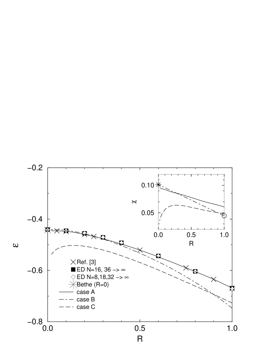
FIG. 1.: $R$-dependence of the ground-state energy per site $\varepsilon$ and the uniform static spin susceptibility $\chi$ (inset).

In order to reduce cluster-shape effects, we use two different groups of clusters of equal symmetry. Our ED data agrees with the Ising-expansion results by Affleck et al. [3] and, in particular, with the Bethe value $\varepsilon(0)=-0.4431$. In the region $R\lesssim 0.25$, the ground-state energy of case B approximately reproduces the exact data. Equivalently, at $R\lesssim 0.25$ the susceptibilities $\chi(R)$ in the cases A and B nearly coincide (see inset of Fig.1).

Our results for the order parameter $m$ plotted in Fig.2 indicate an order-disorder transition at the critical ratio $R_{c}\simeq 0.24$ (note that the cases A and B give very similar results for $R\lesssim 0.25$, cf. also Fig.1). The linear decrease of $m$ with $R$ in the region $0.6\lesssim R\lesssim 1$ in case B is ascribed to the crude (linear) interpolation of $\chi(R)$ in that case. To analyze the ED data for $m^{2}(N)$ calculated by Eq. (6), we use the finite-size scaling arguments given in Refs. [16] and [17] for the 2D (frustrated) Heisenberg antiferromagnet and fit the data to the scaling relation $m^{2}(N)-m^{2}(\infty)\propto N^{-1/2}$ (inset of Fig.2). Thereby, as noted in Ref. [17], the extrapolated $(N\to\infty)$ values for $m$ slightly depend on the factor in front of the sum in Eq. (6): $N^{-1}$ vs. $(N+2)^{-1}$. The finite-size extrapolation of $m$ for $N=16$, 36 depicted in Fig.1 ($1/N$ prefactor) and calculated with an $1/(N+2)$ prefactor agree, at $R=1$, with Ref. [17]. We find a transition to a spin-liquid phase at $R_{c}\simeq 0.24$ or $R_{c}\simeq 0.18$ depending on the chosen prefactor. Let us emphasize the coincidence of the critical coupling ratios obtained in cases A and B, and by Lanczos diagonalizations, where the critical ratio $R_{c}$ turns out to be nearly identical for both cluster sequences.

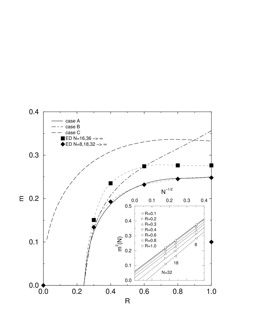
FIG. 2.: Staggered magnetization $m$ for different values of $R$. The short-dashed lines are fits to the ED data using $N=16$, 36 (squares) and tilted $N=8$, 16, 32 (diamonds) clusters with periodic boundary conditions, respectively. The inset demonstrates the deviation of the ED results from the $N^{-1/2}$ scaling law at $R\lesssim 0.3$ (solid lines are least-squares fits).

To illustrate the finite-size scaling in more detail, in the inset of Fig.2 we show the least-squares fits of our ED results. The $N^{-1/2}$ scaling [16], when applied to the small systems (up to $6\times 6$), breaks down for $R\lesssim 0.25$. As recently pointed out by Sandvik [5, 18], at $R\lesssim 0.2$ the QMC simulations reveal an anomalous (non-monotonic) scaling behavior for square lattices, where very large systems are needed to access the $N^{-1/2}$ law indicative of Néel order.

To capture the behavior of $m(R)$ with $R_{c}=0$, let us consider case C. The results for $\varepsilon(R)$ and $\chi(R)$ shown in Fig.1 strongly deviate, in the physically most interesting region of $R$, from those obtained in cases A and B. In particular, at $R\sim 0.2$, $\varepsilon(R)$ and $\chi(R)$ exhibit a strange maximum.

Our findings indicate a rather sharp change in the magnetic properties at $R_{0}\simeq 0.2$. Note that Affleck et al. [3] found a poor convergence of their Padé approximants just below $R\lesssim 0.2$. To shed more light into the crossover at $R_{0}$, we calculate the dependence on $R$ of the two-spin correlation functions depicted in Fig.3.

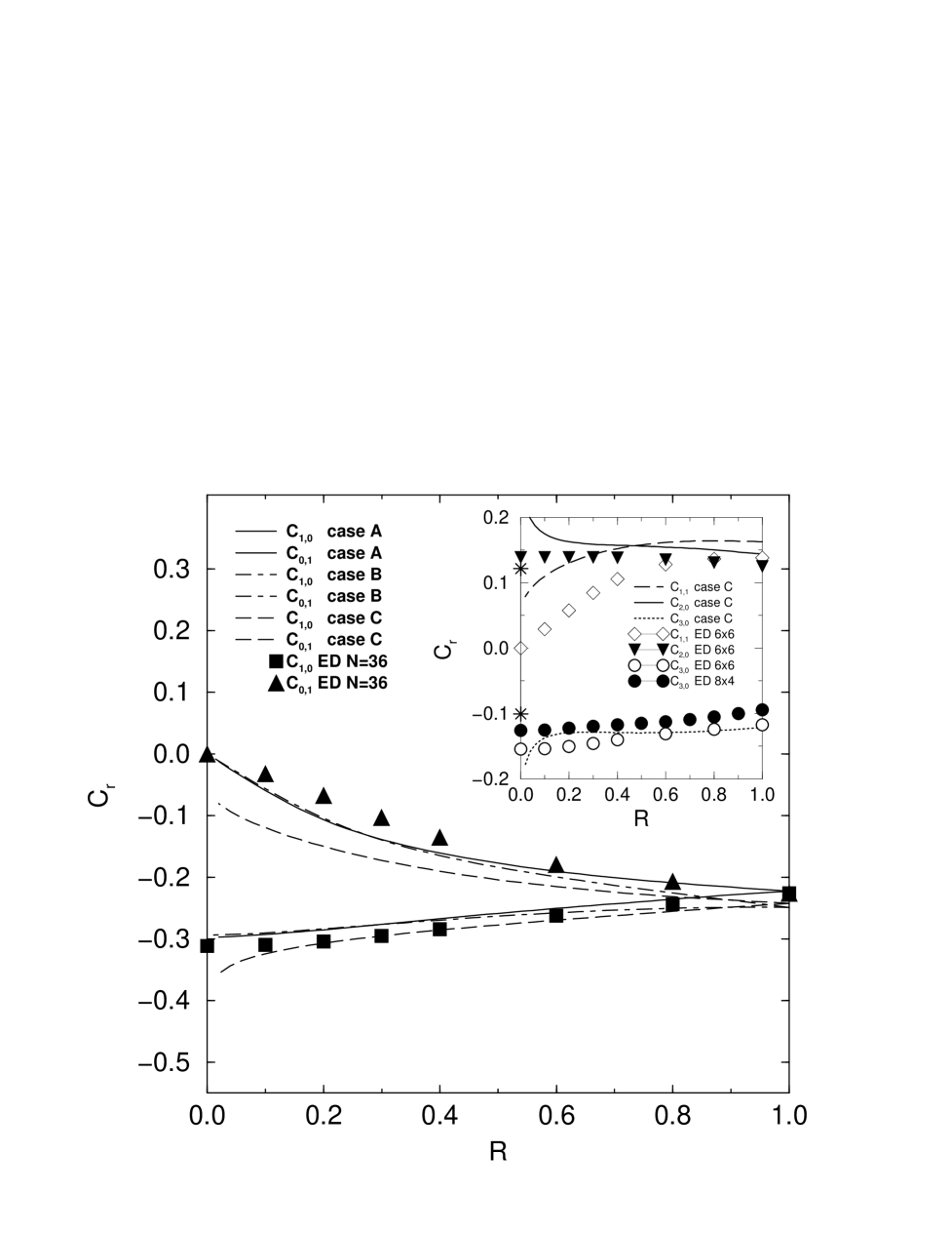
FIG. 3.: NN and longer ranged (inset) spin-correlation functions versus $R$. Theoretical results are compared with ED data obtained for different cluster sizes/shapes. In the inset, at $R=0$, stars denote the extrapolated values of the ED data for chains up to 32 sites using the scaling relation $C_{n,0}(N)-C_{n,0}(\infty)\propto N^{-2}$.

The NN correlation functions in cases A and B reasonably agree with the ED data for a $6\times 6$ system, whereas $C_{0,1}$ in case C notably deviates from those results for $R\lesssim 0.25$. That is, in the $R$ region, where a finite magnetization is incorporated (case C) as compared to the $m=0$ solution in the cases A and B, the SRO is described less well. The same qualitative behavior is found for the correlation functions $C_{1,1}$ and $C_{2,0}$ (see inset of Fig.3): At $R\lesssim 0.25$, the results in cases A and B are in better agreement with ED data than the curve in case C. Note that the ratio $C_{0,1}/C_{1,0}$ determining the anisotropy in the spin-wave velocities according to Eq. (15) does not show a decoupling transition ($C_{0,1}/C_{1,0}=0$) at a finite $R$ value, contrary to the suggestion by Parola et al. [2].

From our results we suggest the following characteristics of the crossover at $R_{0}\simeq 0.2$. In our self-consistent Green’s-function theory the short ranged magnetic correlations, in particular the fluctuations of the correlation functions about their LRO limit, are described rather well. On the other hand, the suppression of LRO by quantum spin fluctuations is overestimated. Moreover, if the correlation functions decrease slowly (subexponentially) towards their long-range limit, our theory does not capture this behavior. Equally, the ED data for the small systems cannot be described by the LRO scaling law $N^{-1/2}$. Our results indicate that this happens for $R<R_{0}\simeq 0.2$. Contrary, at $R>R_{0}$ the decrease of the correlation functions with distance is sufficiently strong so that the LRO limit is nearly reached at relatively short distances. This yields a reasonable scaling behavior of our ED data (inset of Fig.2). To sum up, our results indicate that the crossover at $R_{0}\simeq 0.2$ may be accompanied by a rather sharp change in the spatial dependence of spin correlation functions from strong to weak decrease with distance. At $R<R_{0}$, the system starts to sense the 1D behavior, characterized by an algebraic decrease of the correlation functions.

Finally, in Fig.4 we plot the spin-wave spectrum in the ordered state for the cases A ($R>R_{0}\simeq 0.24$) and C ($R>0$) scaled by $Z_{c}=c_{x}(R=1)/\sqrt{2}$, where $Z_{c}^{A}=1.36$ and $Z_{c}^{C}=1.58$. For $R=1$, in both cases we have $\omega_{\bf q}^{2}=4Z_{c}^{2}(1-\gamma_{\bf q}^{2})$ with $\gamma_{\bf q}=(\cos q_{x}+\cos q_{y})/2$. With decreasing $R$, the anisotropy in $\omega_{\bf q}$ develops gradually, where in case C the 1D limit $\omega_{q_{x}}=2\sqrt{-\alpha_{1}^{x}C_{1,0}}|\sin q_{x}|$ is approached. However, compared with the exact Bethe-ansatz result $\omega_{q_{x}}=\frac{\pi}{2}|\sin q_{x}|$, the spin-wave energy at $q_{x}=\pi/2$ is too high by a factor of about three.

To conclude, the strong evidence for the sharp crossover at the interchain coupling ratio $R_{0}\simeq 0.2$ found by analytical and numerical methods should be corroborated by further QMC studies, especially on the distance dependence of spin correlation functions. This is of particular interest in developing appropriate theories to explain the magnetism in quasi-1D quantum spin systems [9, 11].

FIG. 4.: Spin-wave dispersion $\omega_{\bf q}$ of the 2D spatially anisotropic AFM Heisenberg model along the major symmetry directions of the Brillouin zone.

We thank S.-L. Drechsler, R. Hayn, W. Janke, A. Klümper, J. Stolze, and J. Schliemann for useful discussions. Particularly we are indebted to A. W. Sandvik for putting his (unpublished) QMC data to our proposal. H. F. acknowledges the hospitality at the Universität Leipzig, granted by the graduate college “Quantum Field Theory”. The ED calculations were performed at the LRZ München, HLRZ Jülich, and the HLR Stuttgart.

REFERENCES

- [1] T. Sakai and M. Takahashi, J. Phys. Soc. Jpn. 58, 3131 (1989).
- [2] A. Parola, S. Sorella, and Q. F. Zhong, Phys. Rev. Lett. 71, 4393 (1993).
- [3] I. Affleck, M. P. Gelfand, and R. R. P. Singh, J. Phys. A 27, 7313 (1994); 28 1787 (E) (1995).
- [4] A. Fledderjohann, K.-H. Mütter, M.-S. Yang, and M. Karbach, Phys. Rev. B 57, 956 (1998).
- [5] A. W. Sandvik, cond-mat/9904218.
- [6] U.-J. Wiese and H.-P. Ying, Z. Phys. B 93, 147 (1994).
- [7] A. H. Castro Néto and D. Hone, Phys. Rev. Lett. 76, 2165 (1996); D. Hone and A. H. Castro Néto, J. of Superconductivity 10, 349 (1997).
- [8] N. Majlis, S. Selzer, and G. C. Strinati, Phys. Rev. B 45, 7872 (1992); ibid. 48, 957 (1993).
- [9] H. Rosner, H. Eschrig, R. Hayn, S.-L. Drechsler, and J. Marek, Phys. Rev. B 56, 3402 (1997).
- [10] H. J. Schulz, Phys. Rev. Lett. 77, 2790 (1996); Z. Wang, Phys. Rev. Lett. 78, 126 (1997).
- [11] K. M. Kojima et al., Phys. Rev. Lett. 78, 1787 (1997).
- [12] H. Shimahara and S. Takada, J. Phys. Soc. Jpn. 60, 2394 (1991).
- [13] S. Winterfeldt and D. Ihle, Phys. Rev. B 56, 5535 (1997); ibid. 59, 6010 (1999).
- [14] K. J. Runge, Phys. Rev. B 45, 12292 (1992).
- [15] C. J. Hamer, J. Phys. A 19, 3335 (1986).
- [16] H. Neuberger and T. Ziman, Phys. Rev. B 39, 2608 (1989).
- [17] H. J. Schulz, T. A. L. Ziman, and D. Poilblanc, J. Phys. I France 6, 675 (1996).
- [18] A. W. Sandvik, private communication.