Lattice-dynamics of a disordered solid-solid interface

Abstract

Generic properties of elastic phonon transport at a disordered interface are studied. The results show that phonon transmittance is a strong function of frequency and the disorder correlation length. At frequencies lower than the van Hove singularity the transmittance at a given frequency increases as the correlation length decreases. At low frequencies, this is reflected by different power-laws for phonon conductance across correlated and uncorrelated disordered interfaces which are in approximate agreement with perturbation theory of an elastic continuum. These results can be understood in terms of simple mosaic and two-colour models of the interface.

I Introduction

The transfer of phonons across the interface between two solids is crucial to the operation of a range of novel devices from semiconductor nanostructures, quantum-cascade lasers, vertical structures, superlattices, quantum dot arrays to the cryogenic phonon-mediated detectors of elementary particles. In such structures non-radiative transitions and hot-electron thermalization gives rise to fluxes of highly energetic phonons spanning the whole of the Brillouin zone.

In early studies [1], phonons were regarded as bulk elastic continuum waves so that transmission and reflection of energy at the interface between two materials were a consequence of acoustic mismatch. Such a macroscopic continuum theory describes generic low-frequency properties but does not account for important features such as phonon dispersion, the Debye cutoff and weak bonding at the interface, for which a lattice-dynamical model is required [2]. Most early investigations assume that the solid-solid interface possesses in-plane translational invariance, whereas, it is known that disorder-induced scattering can play a significant role [3, 4]. Within a lowest order perturbation theory [5], it is predicted that disorder can induce a strong frequency dependence in phonon transport coefficients with a power-law crossover determined by interface conditions. The aim of this paper is to go beyond this elastic continuum perturbative approach, by formulating an exact lattice-description valid for terahertz phonon transport, which includes features such as phonon dispersion and singularities in the phonon density of states.

To formulate the problem of phonon transmission (reflection) we consider two identical semi-infinite leads of uniform cross-section attached to a ’scattering region’. The two semi-infinite perfect crystals are treated as waveguides for incident and scattered phonons whose dynamics is described by the lattice equations of motion. The geometry analyzed is shown in Fig.1, where the scattering region consists of a single disordered atomic plane. Disorder at the planar interface is introduced microscopically as correlated or uncorrelated random variation of the on-site atomic masses and we assume that there are no significant anharmonic effects. To calculate transport properties of such a system, we use methods specifically developed to investigate electronic transport through phase-coherent structures [6, 7, 8]. Transport coefficients are calculated as a function of phonon frequency within the Landauer-Buttiker formalism [6] by employing an exact recursive Green function technique [8].

II Details of the calculation

In what follows we present the results for two lattice dynamical models: an fcc lattice with central-force nearest-neighbour interactions and a scalar square lattice. For the former the atomic masses $M_{lmn}$ are located at equilibrium positions ${\bf r}_{lmn}=(la,ma,na)$, where $l,m,n$ sum to an even number and $a{\sqrt{2}}$ is the nearest-neighbour spacing, whereas for the square lattice $a$ is the lattice constant and $n=0$. In the latter case we do not distinguish between phonon polarizations and hence, are not concerned about mode conversion due to scattering.

In the harmonic approximation the linearized equations of motion of an atom located at ${\bf r}_{lmn}$ is

$$M_{lmn}\ddot{u}_{lmn}^{\alpha}=-\sum_{\beta,l^{\prime}m^{\prime}n^{\prime}}K_{lmn,l^{\prime}m^{\prime}n^{\prime}}^{\alpha\beta}u_{l^{\prime}m^{\prime}n^{\prime}}^{\beta},$$ (1)

where $u_{lmn}^{\alpha}$ is the atomic displacement vector,

$$K_{lmn,l^{\prime}m^{\prime}n^{\prime}}^{\alpha\beta} = \kappa(s_{lmn,l^{\prime}m^{\prime}n^{\prime}}^{\alpha}s_{lmn,l^{\prime}m^{\prime}n^{\prime}}^{\beta}-4\delta_{lmn,l^{\prime}m^{\prime}n^{\prime}}\delta^{\alpha\beta}),$$ (2)

$$s_{lmn,l^{\prime}m^{\prime}n^{\prime}}^{\alpha} = \frac{{\bf r}_{l^{\prime}m^{\prime}n^{\prime}}^{\alpha}-{\bf r}_{lmn}^{\alpha}}{\left|{\bf r}_{l^{\prime}m^{\prime}n^{\prime}}-{\bf r}_{lmn}\right|},$$ (3)

and ${\bf r}_{l^{\prime}m^{\prime}n^{\prime}}-{\bf r}_{lmn}$ is taken from the first coordination sphere. The indices $\alpha,\beta$ label the $x,y,z$ components of displacements for the fcc model and should be dropped for the scalar model.

All atoms in the semi-infinite leads are of unit mass, whereas the random masses at the interface have mean value unity and standard deviation $\sigma$. For simplicity we allow the masses to fluctuate only along a single direction, which is chosen to be the [101] and [100] cubic crystallographic directions for the fcc and square lattice respectively. Henceforth, we refer to this as the ’disorder-line’ and denote masses at different positions along the line by $M_{j}$. Thus, even for a three dimensional lattice, due to the residual translational invariance, scattering is confined in the plane fixed by the disorder-line and the angle with respect to the interface determined by the conserved component of the incident phonon momentum. From this point of view our scattering problem is essentialy two dimensional.

An ensemble of $N$ positive masses, where $N$ is the number of atoms along the direction of the disorder-line in the lead cross-section, is generated as follows: First we introduce the correlated random numbers

$$\chi_{j}=\sum_{k}(a_{k}\cos(kj)+b_{k}\sin(kj)),$$ (4)

where $a_{k}$ and $b_{k}$ are Gaussian random numbers with zero mean value and $\langle a_{k}a_{k^{\prime}}\rangle=\langle b_{k}b_{k^{\prime}}\rangle=\delta_{kk^{\prime}}e^{-\frac{k^{2}\xi^{2}}{4}}$. $k$ is taken commensurate with the phonon wavenumbers determined by the boundary conditions in the transverse direction and $\xi$ denotes the correlation length. Random masses $M_{j}$ along the disorder-line with mean value unity and standard deviation $\sigma$ are obtained from $\chi_{j}$ by the linear transformation

$$M_{j}=1+\sigma\cdot\frac{\chi_{j}-\langle\chi_{j}\rangle}{\sqrt{\langle\chi_{j}^{2}\rangle-{\langle\chi_{j}\rangle}^{2}}}.$$ (5)

In order to isolate the effect of correlations, we compare phonon transmission (reflection) coefficients for such correlated interfacial disorder, with those of an uncorrelated disorder configuration obtained by randomly ’shuffling’ the above set.

III S-matrix and phonon interfacial transmittances

In the absence of inelastic scattering, phonon transport through an arbitrary scattering region can be described by the scattering matrix $S$ [6], which depends on the conserved phonon frequency and yields probabilities for all scattering transitions within a system described by a dynamical matrix $D_{lmn,l^{\prime}m^{\prime}n^{\prime}}^{\alpha\beta}=M_{lmn}^{-1/2}K_{lmn,l^{\prime}m^{\prime}n^{\prime}}^{\alpha\beta}M_{l^{\prime}m^{\prime}n^{\prime}}^{-1/2}$. If the scattering region is connected to external reservoirs by phonon waveguides with open channels labelled by quantum numbers $\nu$, then $S$-matrix elements $S_{\nu\nu^{\prime}}(\omega,D)$ are defined such that $|S_{\nu\nu^{\prime}}(\omega,D)|^{2}$ is the outgoing flux of phonons along channel $\nu$, arising from a unit flux incident along channel $\nu^{\prime}$. The scattering matrix defined this way is unitary, i.e., $SS^{\dagger}=1$, and since $S_{\nu\nu^{\prime}}(\omega,D)=S_{\nu^{\prime}\nu}(\omega,D^{\dagger})$, where $D$ is real, $S(\omega,D)$ is symmetric. If $\nu,\nu^{\prime}$ belong to the left (right) lead then the corresponding $S$-matrix elements are left (right) reflection amplitudes which we denote $r_{\nu\nu^{\prime}}=S_{\nu\nu^{\prime}}(r_{\nu\nu^{\prime}}^{\prime}=S_{\nu\nu^{\prime}})$, whereas, if $\nu,\nu^{\prime}$ belong to the right (left) and left (right) lead, the $S$-matrix elements are left (right) transmission amplitudes denoted $t_{\nu\nu^{\prime}}=S_{\nu\nu^{\prime}}(t_{\nu\nu^{\prime}}^{\prime}=S_{\nu\nu^{\prime}})$. It is evident that for an $N^{\prime}$-mode waveguide three distinct transmittances can be defined,

$$T_{\nu\nu^{\prime}}=|t_{\nu\nu^{\prime}}|^{2},\;\;T_{\nu^{\prime}}=\sum_{\nu=1}^{N^{\prime}}|t_{\nu\nu^{\prime}}|^{2},\;\;T=\sum_{\nu,\nu^{\prime}=1}^{N^{\prime}}|t_{\nu\nu^{\prime}}|^{2},$$ (6)

To isolate the frequency dependence of the overall phonon transmittance it is natural to normalize $T$ by the density of states. In the presence of finite-width leads this means averaging $T$ over all open scattering channels $N^{\prime}$ and is equivalent to the angle-averaged transmission coefficient,

$$\langle T(\omega,D)\rangle=T(\omega,D)/{N^{\prime}},$$ (7)

which is related to the corresponding reflection coefficient by

$$\langle R(\omega,D)\rangle=1-\langle T(\omega,D)\rangle.$$ (8)

In what follows the $S$-matrix is obtained by solving Dyson’s equation for the Green function at the surfaces of the two leads [7, 8] (see Fig.1 for definition of L,R), namely

$$G(\omega^{2})=\left(\begin{array}[]{cc}G(L,L;\omega^{2})&G(L,R;\omega^{2})\\ G(R,L;\omega^{2})&G(R,R;\omega^{2})\end{array}\right),$$ (9)

$$G(\omega^{2})=(g(\omega^{2})^{-1}-D_{eff}(\omega^{2}))^{-1},$$ (10)

where $g(\omega^{2})$ is the surface Green function of the semi-infinite leads

$$g(\omega^{2})=\left(\begin{array}[]{cc}g(L,L;\omega^{2})&0\\ 0&g(R,R;\omega^{2})\end{array}\right),$$ (11)

and $D_{eff}(\omega^{2})$ an effective dynamical matrix

$$D_{eff}(\omega^{2})=\left(\begin{array}[]{cc}D_{eff}(L,L;\omega^{2})&D_{eff}(L,R;\omega^{2})\\ D_{eff}(R,L;\omega^{2})&D_{eff}(R,R;\omega^{2})\end{array}\right).$$ (12)

The latter describes the effective (renormalized) coupling between the surfaces of the two leads, obtained by projecting out the internal degrees of freedom of the scatterer using the recursive Green function technique. The Green function $g(\omega^{2})$, the spectrum and structure of the allowed wavequide modes at fixed phonon density of states, as well as $S(\omega,D)$ are calculated using a general algorithm developed in Ref. [8].

IV Phonon transmittance at low frequencies

We present results for the average transmission coefficient $\langle T(\omega)\rangle_{c}$ where the subscript c denotes a configurational averaging. In Fig.2(a),(b) the frequency dependence of the overall transmission coefficient $\langle T(\omega)\rangle_{c}$ averaged over 10 realizations of the interfacial mass-disorder for the fcc lattice and over 500 for the scalar square lattice is shown. The width of the disorder-line is 29 and 100 nearest-neighbour spacings respectively, which corresponds to $3\times 29$ and $1\times 100$ degrees of freedom.

For the fcc model periodic boundary conditions in the lateral direction (disorder-line) were used, whereas for the scalar model we adopted fixed-end boundary conditions. The boundary conditions set the precise frequencies at which propagating waveguide modes become available in the external leads, but apart from features which scale inversely with the number of such modes do not affect the shape of the transmittance curves. Figure 2 shows that for both fcc and scalar lattices, phonon transmittances (reflectances) follow the same universal behaviour. At sufficiently low frequencies, the phonon transmittance for correlated disorder is lower than for uncorrelated interfacial disorder with the same mean mass and standard deviation $\sigma$.

At low frequencies the results of lattice-dynamical calculations in Fig.2(a),(b) are in good agreement with perturbation theory [5]. To model the disorder in [5] a thin layer of dissimilar material sandwiched between irregular boundaries was introduced. The density and elastic constants of this layer were assumed to differ from those of the bulk on either side of the layer. To make a comparison with the perturbative analysis we consider the case of no fluctuation in the elastic constants and a line of random masses at the location of the idealized interfacial plane $z=0$, i.e., $\Delta\rho({\bf x},z)=\Delta\rho\zeta({\bf x})\delta(z)=\Delta\rho({\bf x})\delta(z)$, with $\zeta({\bf x})$ a random function of lateral coordinate with zero mean value. Apart from lattice discreteness which plays no significant role in the long-wavelength limit there is no difference between our model of site-to-site mass disorder and the model of interfacial roughness of Ref. [5]. The following relation is useful when comparing the results

$$\langle{\left(\frac{\Delta M_{j}}{M}\right)}^{2}\rangle={\sigma}^{2}=\left(\frac{\Delta\rho}{\rho}\right)^{2}\;\frac{\langle{\zeta}^{2}\rangle}{a^{2}}.$$ (13)

For such a two dimensional model the perturbation theory [5] with uncorrelated disorder $\xi=a$ and $k\xi\ll 1$, where k is the phonon wavevector, yields

$$\langle T(\omega)\rangle_{c}^{unc}=1-\pi^{\frac{5}{2}}\;\sigma^{2}\;\left(\frac{\omega}{\omega_{max}}\right)^{3},$$ (14)

while for correlated disorder at sufficiently high frequencies so that $k\xi\gg 1$ the perturbative result is

$$\langle T(\omega)\rangle_{c}^{cor}=1-\pi^{2}\;\sigma^{2}\;\left(\frac{\omega}{\omega_{max}}\right)^{2}.$$ (15)

More generally for all $\omega$, Fig.2(c) shows the perturbative results for $\xi\rightarrow 0$ and $\xi\rightarrow\infty$. Equations (14) and (15) are in good agreement with the exact lattice-dynamical calculation. They both show lower transmittance for correlated disorder over a wide range of frequencies until the faster power dependence of phonon transmittance for uncorrelated disorder causes the two curves to cross at a frequency $\omega^{\star}$. According to the perturbative calculations $\omega^{\star}$ should be close to half the maximum phonon frequency $\omega_{max}$ independent of disorder characteristics, correlation length and strength. Despite the similarities, this is not evident in the lattice-dynamical calculations. Indeed, the crossing point is quite close to a singularity in the phonon density of states and thus using an elastic continuum model at frequencies of order $\omega^{\star}$ is an oversimplification.

Another simplifying assumption of the theory in Ref.[5] is the neglect of multiple scattering. This gives the power law $\langle R(\omega)\rangle_{c}^{unc}\sim\omega^{d+1}$ (Rayleigh scattering) with subsequent decrease by one (two) power(s) for correlated disorder in 2D (3D). A log-log plot of phonon reflectances showed that both lattice dispersion and multiple phonon scattering effects result in a change of the power exponents to a slightly different value. However, the drop by approximately one power for our 2D scattering problem in the case of correlated disorder prevails in all cases. The effect is attributed to the restrictions in the phase volume available for the scattered states, due to the correlation-induced finite width of the disordered spectral distribution.

V Spectral properties of phonon transmittance

Phonon transmittances over the whole frequency spectrum for the scalar model for two different values of disorder strength $\sigma$ are shown in Fig.3. In addition to the low frequency behaviour discussed in Sec. IV, the transmittance shows a cusp at a frequency corresponding to a van Hove singularity in the phonon density of states and rapidly drops to zero at the maximum frequency of the phonon spectrum $\omega_{max}$. At the van Hove singularity the difference between correlated and uncorrelated disorder realizations is much less pronounced. All these features are also seen for the fcc model but the exact behaviour at van Hove singularities is less clear due to the finite-size effects described in the previous section. To interpret the results we concentrate on the scalar model.

The general expression for the transmission amplitude from incident channel $\nu^{\prime}$ to channel $\nu$ for systems with nearest-neighbour interactions has been derived in [8]. The explicit expression for the scalar model with periodic boundary conditions is

$$t_{\nu\nu^{\prime}}=\frac{1}{N}(\sum_{m,m_{1},m^{\prime}=1}^{N}e^{-ik_{\nu}^{y}ma}G_{LR}(m,m_{1})W(m_{1},m^{\prime})e^{ik_{\nu^{\prime}}^{y}m^{\prime}a)})\sqrt{\frac{v_{\nu}}{v_{\nu^{\prime}}}}e^{-ik_{\nu}^{x}a}.$$ (16)

Here ${v_{\nu}}$ is the component of the group velocity in x-direction along the lead axis of the $\nu$-th channel mode, m labels sites at the interface (along lateral direction), and $G_{LR}$ has been defined in Eq.(9). The matrix W is given by [8]

$$W(m_{1},m^{\prime})=\frac{\omega_{max}^{2}}{8N}\sum_{\mu=1}^{N}e^{ik_{\mu}^{y}(m_{1}-m^{\prime})a}(e^{ik_{\mu}^{x}a}-e^{-ik_{\mu}^{x}a}).$$ (17)

In formulae (16,17), $k_{\nu}^{y}=\frac{2\nu\pi}{Na}$, as a result of transverse quantization with periodic boundary conditions, while $k_{\nu}^{x}$ denotes the wavenumber along the lead axis for phonons of fixed frequency $\omega$ of state $\nu$ ($\nu$-th channel).

Using the complete orthonormalized set of functions $\{\frac{1}{\sqrt{N}}e^{ik_{\mu}^{y}ja}\}$ describing the profile of modes in the transverse direction, $G_{LR}(m,m_{1})$ can be written

$$G_{LR}(m,m_{1})=\frac{1}{N}\sum_{\mu,\mu^{\prime}=1}^{N}e^{ik_{\mu}^{y}ma}G_{LR}(\mu,\mu^{\prime})e^{-ik_{\mu^{\prime}}^{y}m_{1}a}.$$ (18)

By substitution of Eq.(17),(18) to (16) one obtains

$$t_{\nu\nu^{\prime}}=\frac{\omega_{max}^{2}}{4}G_{LR}(\nu,\nu^{\prime})\;i\;sin(k_{\nu^{\prime}}^{x}a)\sqrt{\frac{v_{\nu}}{v_{\nu^{\prime}}}}e^{-ik_{\nu}^{x}a}.$$ (19)

Thus, to calculate the channel-to-channel transmittance ${\langle T_{\nu\nu^{\prime}}\rangle}_{c}={\langle|t_{\nu\nu^{\prime}}|^{2}\rangle}_{c}$ or generally the overall transmittance ${\langle T\rangle}_{c}$ one needs to consider the non-trivial statistically averaged product of two Green functions, ${\langle G_{LR}(\nu,\nu^{\prime})G_{LR}^{\ast}(\nu,\nu^{\prime})\rangle}_{c}$ or ${\langle G_{LR}(m,m^{\prime})G_{LR}^{\ast}(s,s^{\prime})\rangle}_{c}$.

In what follows, we shall demonstrate that generic features can be captured by considering the case of a regular array of atoms with mass $M^{\prime}$ located at the interface, thereby forming a linear(planar) defect in a two(three) dimensional system.

In this case, the full Green function $G_{LR}(\nu,\nu^{\prime})$ is of the form

$$G_{LR}(\nu,\nu^{\prime})=\frac{g_{o}(\nu,\nu^{\prime})e^{ik_{\nu^{\prime}}^{x}a}}{1-\sigma^{\prime}\omega^{2}g_{o}(\nu,\nu^{\prime})},$$ (20)

where $g_{o}(\nu,\nu^{\prime})=-4i\delta_{\nu,\nu^{\prime}}/(\omega_{max}^{2}sin(k_{\nu^{\prime}}^{x}))$ is the Green function of the infinite ideal lead at coinciding arguments, and $\sigma^{\prime}=\frac{M^{\prime}-M}{M}$ is the relative mass difference at the location of the defects. Substituting this result into Eq.(7) and (19) yields for the transmittance

$$\langle T\rangle=\frac{1}{N^{\prime}}\sum_{\nu(open)}\frac{sin^{2}(k_{\nu}^{x}a)}{sin^{2}(k_{\nu}^{x}a)+{\sigma^{\prime}}^{2}(\frac{2\omega}{\omega_{max}})^{4}}$$ (21)

Eq.(21) exhibits the following features: (i)$\langle T\rangle$ equals unity for an ideal interface with $\sigma^{\prime}=0$. (ii)At low frequencies both $\omega,k_{\nu}^{x}\rightarrow 0$, $sin(k_{\nu}^{x}a)\sim\omega$ and therefore $\langle T\rangle\rightarrow 1-\alpha\omega^{2}$, where $\alpha$ is numerical coefficient, in full agreement with the results of perturbation theory [5] and formula (15). (iii)At the end of the phonon spectrum $\langle T\rangle\rightarrow 0$ since propagating channels are closing with $sin(k_{\nu}^{x}a)$ approaching zero at the Brillouin zone boundaries. This effect is analogous to the total reflection by a single mass defect in one dimension. (iv)At the van Hove singularity all channels are open and Eq.(21) reduces to

$$\langle T\rangle=\frac{1}{N}\sum_{\nu=1}^{N}\frac{sin^{2}(\frac{2\nu\pi}{N})}{sin^{2}(\frac{2\nu\pi}{N})+4{\sigma^{\prime}}^{2}},$$ (22)

which suggests that for $\sigma^{\prime}<1$ the dependence on disorder strength is much weaker than at low frequencies. Also, $sin(k_{\nu}^{y}a)$ is small for a large number of contributing channels thereby yielding the characteristic cusp. (v)We also note that Eq.(21) has been derived for the [100] orientation of the interface but since the phonon group velocity along the lead axis is proportional to $sin(k_{\nu}^{x}a)$ the transmittance is in general anisotropic.

In Fig.4(a), we plot the phonon transmittance given by formula (21) for selected values of $\sigma^{\prime}$ along with the numerical results for correlated disorder realizations. Notice that in spite of the differences in the type of interfacial defect the curves look very similar. A natural way to explain this result is to view the interface for correlated disorder as a mosaic of clusters of average diameter $\sim\xi$. Suppose that within a particular cluster $i$ all sites are occupied by defects with the same mass and characteristic relative mass difference $\sigma^{\prime}_{i}$. As long as the phonon wavelength is smaller than the correlation length, i.e., $k\xi\gg 1$, the overall transmittance can be considered as the average over all clusters with local transmittances given by Eq.(21). In Fig.4(b) such an average is plotted for clusters with excess mass fully balanced by clusters with mass deficit. The relative mass difference is taken from a Gaussian distribution with width equal to the disorder strength $\sigma$. Clearly, this procedure gives a better fit to the correlated disorder curve, which suggests that the phonon transmittance across a correlated disordered interface can be split to a statistically averaged mean field contribution induced by mosaic grains and a fluctuating component. The latter is controlled by the rapid residual variations in the relative mass difference at the cluster boundaries as well as the fluctuations in cluster sizes.

The qualitative agreement between correlated disorder realizations and the mosaic picture prompts us to ask whether there exists a simple model for the case of uncorrelated disorder. To explore this possibility, we examine a two-colour disorder model where linear interfacial defects are built up from atoms with relative mass difference $\sigma^{\prime}$ which alternates sign every $L/a$ sites. This model is motivated by the observation that uncorrelated disorder contains all spatial harmonics with equal probability. In what follows, we compare the exact transmittance for uncorelated disorder with that of the two-colour model, averaged over many values of $L$. In Fig.5, we plot the mean arithmetic value of the phonon transmittances for $L=2,4,..,10a$ taken after averaging over 500 two-colour disorder realizations given by a Gaussian distribution with zero mean and $\sqrt{\langle{\sigma^{\prime}}^{2}\rangle}=\sigma$. The remarkable agreement with the calculations for the uncorrelated disorder over a wide range of frequencies suggests that the mean field contribution for this case can be calculated by picking up few elements from the basis set of the two-colour disorder model.

Finally, we compare the results of our calculation with the diffuse mismatch model DMM introduced in [9] and extensively used in studies of Kapitza conductance [4, 9, 10]. Application of the DMM at a boundary between two solids with identical acoustic properties gives a $50\%$ phonon transmittance independent of frequency. It can be easily demonstrated that the Kapitza conductance $\sigma_{K}$ for our model is larger than that predicted by the DMM. It is also less than the radiation limit which in this case would coincide with acoustic mismatch theory (total transmission). Moreover, $\sigma_{K}$ is larger for uncorrelated disorder than for correlated. Finally, one notes that the results of [2] which are valid for phonon transmission through the ideal interface between two different fcc crystals a transmittance which is frequency-independent over the whole spectrum up to a cut-off frequency corresponding to maximum phonon frequency in one of the crystals, whereas, in our model the phonon transmittance is a strong function of frequency.

VI Summary

In summary, generic properties of elastic phonon transport at a disordered interface were studied by computing the exact scattering properties of a single disordered atomic layer sandwiched between identical waveguides. The results show that phonon transmittance is a strong function of frequency and the disorder correlation length. At frequencies lower than the van Hove singularity the transmittance at a given frequency increases as the correlation length decreases. At low frequencies, this is reflected by different power-laws for phonon conductance across correlated and uncorrelated disordered interfaces which are in approximate agreement with perturbation theory of an elastic continuum [5]. We also investigated simple mosaic and two-colour models of the interface and showed that phonon transmittance through interfaces with correlated and uncorrelated disorder can be understood in terms of phonon conductances of structures with regular interfaces.

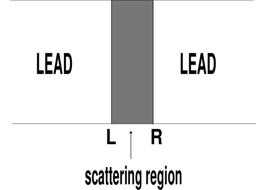
FIG. 1.: A typical scattering geometry, where L(R) refer to sites on the faces of left(right) lead.

FIG. 2.: Phonon transmittance for the (a)fcc model($\xi=5.65$), (b)square scalar model($\xi=20$), (c)estimates based on perturbation theory. In the (a) and (b) insets the corresponding normalised DOS versus $\omega$ is plotted. Frequency is measured in units of $\sqrt{\kappa/m}$. Inset (c) shows a single realization of $m_{j}$ versus j for a line of correlated and uncorrelated masses($\sigma=0.3$ in all plots).

FIG. 3.: Phonon transmittance for $\sigma=0.3$ and $0.1$. Curves (1), (2) correspond to correlated ($\xi=15$) and uncorrelated disorder for $\sigma=0.3$, whereas curves (3), (4) are for $\sigma=0.1$.

FIG. 4.: Phonon transmittance for correlated disorder and regular models as explained in the text. In both (a) and (b) curves (1) and (3) correspond to correlated disorder for $\sigma=0.3$ and $0.1$ ($\xi=15$). In (a), curves (2) and (4) are for the regular interlayer with $\sigma^{\prime}=0.3$ and $0.1$. The results of the mosaic model are shown in (2b) and (4b).

,

FIG. 5.: Phonon transmittance for uncorrelated disorder, curves (1) and (3) for $\sigma=0.3$ and $0.1$, and the two-colour disorder model.

REFERENCES

- [1] W.A. Little, Can. J. Phys. 37 (1959) 5080
- [2] D.A. Young and H.J. Maris, Phys. Rev. B 40 (1989) 3685
- [3] M.N. Wybourne and J.K. Wigmore, Rep. Prog. Phys. 51 (1988) 923
- [4] E.T. Swartz, R.O. Pohl, Rev. Mod. Phys. 61 (1989) 605
- [5] A.G. Kozorezov et al, Phys. Rev. B 57 (1998) 7411
- [6] M. Büttiker, Y. Imry, R. Landauer, S. Pinhas, Phys. Rev. B 31 (1985) 6207, and refs therein
- [7] C.J. Lambert, V.C. Hui and S.J. Robinson, J. Phys. : Condens. Matter 5 (1993) 4187
- [8] S. Sanvito, C.J. Lambert, J.H. Jefferson, A.M. Bratkovsky, submitted to Phys. Rev. B, also available on cond-mat/9808282
- [9] E.T Swartz and R.O. Pohl, Appl. Phys. Lett. 51 (1987) 2200
- [10] R.J. Stoner and H.J. Maris. Phys. Rev. B 48 (1993) 16373
,