Diffusion of two repulsive particles in a one-dimensional lattice

Abstract

The problem of the lattice diffusion of two particles coupled by a contact repulsive interaction is solved by finding analytical expressions of the two-body probability characteristic function. The interaction induces anomalous drift with a vanishing velocity, the average coordinate of each particle growing at large times as $t^{1/2}$. The leading term of the mean square dispersions displays normal diffusion, with a diffusion constant made smaller by the interaction by the non-trivial factor $1-1/\pi$. Space continuous limit taken from the lattice calculations allows to establish connection with the standard problem of diffusion of a single fictitious particle constrained by a totally reflecting wall. Comparison between lattice and continuous results display marked differences for transient regimes, relevant with regards to high time resolution experiments, and in addition show that, due to slowly decreasing subdominant terms, lattice effects persist even at very large times.

I Introduction

Whereas classical ordinary diffusion of a single particle is universally known, diffusion of interacting particles does not seem to have drawn much attention. A notable exception is the seminal paper by Fisher [1], which introduces basic ideas and solves, in various cases, the problem of finding the probability for the reunion of a given number of “drunken walkers” wandering on a one-dimensional lattice. The so-called tracer problem also received some attention, following the solution given by Harris [2] for the $1d$ case (recent bibliography on this subject can be found in Mallick’ thesis [3]). More recently, intensive work [4], [5] and references therein, has been done one the asymmetric simple exclusion process ([6]) which describes the biased motion of a lattice gas with hard-core interaction.

The interaction between diffusing particles appears to be relevant in many fields: one-dimensional hopping conductivity [7], ion transport in biological membranes [8], [9], channelling in zeolithes [10]. Generally speaking, the interactions are expected to play a dominant role in low-dimensionality systems and/or sytems with geometrical constraints. Such problems have been analyzed in the continuous space limit of the so-called single-file model [11], [12].

I here consider one of the simplest problems, namely that of two diffusing particles on a $1d$-lattice with a repulsive contact interaction, by directly solving the lattice master equation using elementary methods and obtaining the exact two-body probability at all times; this allows to find the behaviour $\forall\,t$ of the mean square dispersion of the coordinates. The totally asymmetric version of this problem (directed random walk in which each particle can move only in one direction) was treated in ref. [5] using a Bethe ansatz; among other results, these authors gave explicit asymptotic behaviour of the two first moments of the coordinates in the case of two diffusing particles.

The continuous space limit of the model here considered is simply related to the problem of a single fictitious particle subjected to a perfectly reflecting barrier, as shown below. On the other hand, working on a lattice seems to be usually the most natural approach on physical grounds and is even a necessity when no continuous limit exists; an example of such a situation is the pure growth problem, equivalent to a directed walk, for which continuous limit of the master equation generates a purely mechanical Liouville equation, in which diffusive effects have disappeared [13]. When the continuous limit exists, it is expected on physical grounds that both versions provide essentially the same results in the long time limit, when part of the microscopic details become irrelevant. Nevertheless, although leading terms are expected to coincide, subdominant corrections may play a rather important role, as shown below, since they usually follow power-laws in time with small exponents entailing that corrections are long-lived. When the relevant experimental timescale is short, results obtained by scaling hand-waving asymptotic arguments are of little physical interest and continuous models may even display serious shortcomings : as an example, as shown below, the velocity at short times turns out to be infinite in the continuous approximation whereas its lattice analogue is perfectly well defined and is finite. In addition, somewhat surprinsingly, lattice effects persist even in the final regime, as constrasted to the ordinary diffusion of a single particle. This is why, as a whole, lattice models in continuous time are worthy to investigate: the discreteness of space, appearent in the transient as well as in the long-time dynamics, is not a minor feature of the problem. To be sure, lattice problems are by nature less “universal” than continuous ones in the sense that most results obtained in such a framework usually depend on microscopic details such as the lattice structure ([14]); nevertheless, they usually contain much more physically relevant information than continuous ones and, as such, can suggest high-resolved in time new experiments.

II The model

The basic assumptions of the present lattice model are as follows : i) at some time ($t=0$), a pair of particles is located on two given adjacent lattice sites labelled $n=0$ and $1$. ii) when separated by more that one lattice spacing, each member of the pair has a symmetric diffusive motion, independently of the other; for simplicity, it is assumed that hopping can occur between one site and its nearest-neighbours. The hopping probability per unit time is denoted as $W$ and allows to define a diffusion constant $D=a^{2}W$, $a$ being the lattice spacing and $W^{-1}$ the diffusion time. iii) when the two particles are located on two adjacent sites, each of them can only move onto the empty available site: this models the contact interaction. As a consequence, the two particles cannot stand on the same site and cannot cross each other. Any initial condition thus definitely induces a left-right symmetry breaking. Conventionally, with the above initial condition, the particle located at $n=0$ (resp. $n=1$) at time $t=0$ will be given the label $1$ (resp. $2$).

With these assumptions, the master equation (M. E.) for the probability $p_{n,m}(t)$ to find the two particles located on sites $n$ and $m$ at time $t$ can be written following the standard procedure. One first considers the evolution of $p_{n,m}(t)$ between $t$ and $t+\Delta t$, where $\Delta t$ is a finite time interval, by exhausting all basic elementary jumps and expressing their probabilities in terms of the products $W\Delta t$; by forming the difference $p_{n,m}(t+\Delta t)-p_{n,m}(t)$, by dividing both sides by $\Delta t$ and taking the limit $\Delta t\rightarrow 0$, one eventually obtains the time-continuous following M. E. ($\delta_{n,m}$ is the Kronecker symbol):

$$\frac{{\rm d}}{{\rm d}t}\,p_{n,m}\, = \,-\,2W\,\left[2-(\delta_{n,m+1}+\delta_{n,m-1})\right](1-\delta_{n,m})\,p_{n,m}+\,W\,(p_{n+1,m}+p_{n,m-1})(1-\delta_{n,m-1})\,(1-\delta_{n,m})$$ (2.1)

$$+ \,W\,(p_{n-1,m}+p_{n,m+1})(1-\delta_{n,m+1})\,(1-\delta_{n,m})\enspace.$$ (2.2)

In such a way, as usual, all elementary steps involving two or more steps disappear (their probabilities scale as $(\Delta t)^{k}$ with $k\geq 2$). The $(1-\delta_{nm})$ factors account for the fact that the two particles cannot stand on the same site: when $p_{nn}(0)=0$ – which is the case for the chosen initial condition –, then $p_{nn}(t)$ remains equal to zero at all times.

Our aim is to solve eq. (2.2) in order to deduce the full probability distribution $\{p_{n,m}(t)\}$ and the related one-body (marginal, reduced) distributions $\{p_{n}(1,t)\}$ and $\{p_{m}(2,t)\}$ given by:

$$p_{n}(1,t)\,=\,\sum_{m=-\infty}^{+\infty}p_{n,m}(t)\hskip 28.45274ptp_{m}(2,t)\,=\,\sum_{n=-\infty}^{+\infty}p_{n,m}(t)\enspace.$$ (2.3)

Eq. (2.2) can be solved by first introducing the generating (characteristic) function $f(\phi,\psi,t)$ defined as:

$$f(\phi,\psi,t)\,=\,\sum_{n,m=-\infty}^{+\infty}p_{n,m}(t)\,{\rm e}^{\rm in\phi}\,{\rm e}^{\rm im\psi}\enspace.$$ (2.4)

allowing to find each $p_{n,m}$ by inverse Fourier transformation or to get the marginal distributions by setting one of the arguments $\phi$ or $\psi$ equal to zero, and to find directly all the moments by successive derivations. It is readily seen that the characteristic function $f$ satisfies the following homogeneous integro-differential equation:

$$\frac{\partial}{\partial t}f(\phi,\psi,t)\, = \,-2W(2-\cos\phi-\cos\psi)f(\phi,\psi,t)+2W\,\int_{0}^{2\pi}\,\frac{{\rm d}\phi^{\prime}}{2\pi}\,[2-\cos\phi^{\prime}-\cos(\phi+\psi-\phi^{\prime})]f(\phi^{\prime},\phi+\psi-\phi^{\prime},t)$$ (2.5)

$$+ 2W\,\int_{0}^{2\pi}\,\frac{{\rm d}\phi^{\prime}}{2\pi}\,[2-\cos(\phi-\phi^{\prime})-\cos\phi-\cos\psi]f(\phi^{\prime},\phi+\psi-\phi^{\prime},t)\enspace.$$ (2.6)

The above stated initial condition writes $f(\phi,\psi,t=0)={\rm e}^{\rm i\psi}$ and entails that $p_{n,m}(t)=0$ for $n\geq m$. By subsequently making a Laplace transformation:

$$f_{\rm L}(\phi,\psi,z)\,=\,\int_{0}^{+\infty}\,{\rm d}t\,{\rm e}^{-zt}f(\phi,\psi,t)\enspace,$$ (2.7)

it is found that the function $f_{\rm L}$ obeys the following homogeneous integral equation:

$$zf_{\rm L}(\phi,\psi,z)\,-\,{\rm e}^{\rm i\psi}\, = \,-2W(2-\cos\phi-\cos\psi)f_{\rm L}(\phi,\psi,z)+2W\,(2-\cos\phi-\cos\psi)\int_{0}^{2\pi}\,\frac{{\rm d}\phi^{\prime}}{2\pi}\,f_{\rm L}(\phi^{\prime},\phi+\psi-\phi^{\prime},z)$$ (2.8)

$$+ 4W\,(\sin\phi-\sin\frac{\phi+\psi}{2}\,\cos\frac{\phi+\psi}{2})\,\int_{0}^{2\pi}\,\frac{{\rm d}\phi^{\prime}}{2\pi}\,\sin\phi^{\prime}\,f_{\rm L}(\phi^{\prime},\phi+\psi-\phi^{\prime},z)$$ (2.9)

$$+ 4W\,(\cos\phi-\cos^{2}\frac{\phi+\psi}{2})\int_{0}^{2\pi}\,\frac{{\rm d}\phi^{\prime}}{2\pi}\,\cos\phi^{\prime}\,f_{\rm L}(\phi^{\prime},\phi+\psi-\phi^{\prime},z)\enspace.$$ (2.10)

This is a Fredholm equation with a degenerate kernel; as such, its solution is a linear combination of the three auxiliary quantities $M(\theta)$, $X(\theta)$ and $Y(\theta)$ ($\theta=\phi+\psi$) defined as:

$$M(\theta)\, = \,\int_{0}^{2\pi}\,\frac{{\rm d}\phi^{\prime}}{2\pi}\,f_{\rm L}(\phi^{\prime},\phi+\psi-\phi^{\prime},z)$$ (2.11)

$$X(\theta)\, = \,\int_{0}^{2\pi}\,\frac{{\rm d}\phi^{\prime}}{2\pi}\,\cos\phi^{\prime}\,f_{\rm L}(\phi^{\prime},\phi+\psi-\phi^{\prime},z)$$ (2.12)

$$Y(\theta)\, = \,\int_{0}^{2\pi}\,\frac{{\rm d}\phi^{\prime}}{2\pi}\,\sin\phi^{\prime}\,f_{\rm L}(\phi^{\prime},\phi+\psi-\phi^{\prime},z)$$ (2.13)

$M$, $X$ and $Y$ satisfy an inhomogeneous system which can be written down after a somewhat lengthy but straightforward calculation:

$$(1-c_{11})M-c_{12}X-c_{13}Y=c_{10}$$ (2.14)

$$-c_{21}M+(1-c_{22})X-c_{23}Y=c_{20}$$ (2.15)

$$-c_{31}M-c_{32}X+(1-c_{33})Y=c_{30}$$ (2.16)

where the various coefficients are equal to:

$$c_{10} = \frac{{\rm e}^{\rm i\theta/2}\,{\rm e}^{-u}}{4W\cos(\theta/2)\,\sinh u}\hskip 40.0ptc_{20}=\frac{{\rm e}^{\rm i\theta}+{\rm e}^{-2u}}{8W\mid\cos(\theta/2)\mid\,\sinh u}\hskip 40.0ptc_{30}=\frac{{\rm e}^{\rm i\theta}-{\rm e}^{-2u}}{8\rm iW\mid\cos(\theta/2)\mid\,\sinh u}$$ (2.17)

$$c_{11} = \frac{1-{\rm e}^{-u}\mid\cos(\theta/2)\mid}{\mid\cos(\theta/2)\mid\,\sinh u}\hskip 40.0ptc_{12}=\frac{{\rm e}^{-u}-\mid\cos(\theta/2)\mid}{\sinh u}\hskip 60.0ptc_{13}=\frac{\tan(\theta/2)}{\sinh u}({\rm e}^{-u}-\mid\cos(\theta/2)\mid)$$ (2.18)

$$c_{21} = \frac{{\rm e}^{-u}}{\sinh u}(1-\cosh u\,\mid\cos(\theta/2)\mid)\hskip 90.0ptc_{22}={\rm e}^{-u}\,\frac{\sinh u+\cos^{2}(\theta/2)\,({\rm e}^{-u}-\mid\cos(\theta/2)\mid)}{\mid\cos(\theta/2)\mid\sinh u}$$ (2.19)

$$c_{23} = c_{32}=\frac{{\rm e}^{-u}\sin(\theta/2)}{2\sinh u\,\mid\cos(\theta/2)\mid}({\rm e}^{-u}-\mid\cos(\theta/2)\mid)\hskip 40.0pt$$ (2.20)

$$c_{31} = \frac{{\rm e}^{-u}\tan(\theta/2)}{\sinh u}(1-\cosh u\,\mid\cos(\theta/2)\hskip 70.0ptc_{33}={\rm e}^{-u}\,\frac{\sinh u+\sin^{2}(\theta/2)\,({\rm e}^{-u}-\mid\cos(\theta/2)\mid)}{\mid\cos(\theta/2)\mid\sinh u}$$ (2.21)

In these equations, the quantity $u$ is defined as follows:

$$\cosh u\,=\,\frac{z+4W}{4W\,\mid\cos(\theta/2)\mid}\enspace.$$ (2.22)

$u$ is a function of $z$ and $\theta$, uniquely defined by continuity from the branch assuming real positive values when $z$ is a real positive number.

The solution of the above system allows eventually to write down the Laplace transform of the generating function (2.7) as the following ($Z=z/4W$) :

$$f_{\rm L}(\phi,\psi,z)\,=\,\frac{1}{4W}\,\frac{{\rm e}^{\rm i\psi}\,\mid\cos\frac{\phi+\psi}{2}\mid}{Z+1-\frac{1}{2}(\cos\phi+\cos\psi)}\,\frac{R(\phi+\psi,Z)\,{\rm e}^{\rm i(\phi-\psi)/2}-\mid\cos\frac{\phi+\psi}{2}\mid}{R(\phi+\psi,Z)-\cos^{2}\frac{\phi+\psi}{2}}\enspace,$$ (2.23)

where:

$$R(\theta,Z)\,\,=\,Z+1-\left[(Z+1)^{2}-\cos^{2}(\theta/2)\right]^{1/2}\enspace.$$ (2.24)

This is a first writing of the full solution of the present problem, since it allows to find all the moments of the two-body distribution $\{p_{n,m}(t)\}$ in their Laplace representation. In addition, Laplace inversion of eq. (2.23) gives the characteristic function in the time domain:

$$f(\phi,\psi,t)\,\, = \,{\rm e}^{i\psi}\,\frac{\beta(1-\alpha){\rm e}^{i(\phi-\psi)/2}+\beta^{2}-\alpha}{\beta^{2}-2\alpha+1}\,{\rm e}^{4(\alpha-1)Wt}$$ (2.25)

$$+ \,{\rm e}^{i\psi}\,(1-\beta\,{\rm e}^{i(\phi-\psi)/2})\,{\cal P}\int_{-\beta}^{+\beta}\frac{dx}{\pi}\frac{{\rm e}^{4Wt(x-1)}}{x-\alpha}\frac{(\beta^{2}-x^{2})^{1/2}}{\beta^{2}-2x+1}\enspace.$$ (2.26)

In eq. (2.26), ${\cal P}$ denotes the Cauchy principal part and :

$$\alpha\,=\,\cos\frac{\phi+\psi}{2}\,\cos\frac{\phi-\psi}{2}\hskip 28.45274pt\beta\,=\,\mid\cos\frac{\phi+\psi}{2}\mid\enspace.$$ (2.27)

Moreover, by setting $\psi=0$ (resp $\phi=0$) in eq. (2.23) one readily obtains the Laplace transform of the characteristic function for the reduced (marginal) one-body distribution for the particle labelled $1$ (resp. $2$), $f_{1,\,\rm L}(\phi,z)$ (resp. $f_{2,\,\rm L}(\psi,z)$); their expressions for $-\pi\leq\phi\leq+\pi$ writes:

$$f_{1,\,\rm L}(\phi,z)\,\frac{1}{4W}\,\frac{\cos\frac{\phi}{2}}{Z+\sin^{2}\frac{\phi}{2}}\,\frac{R(\phi,Z)\,{\rm e}^{\rm i\phi/2}-\cos\frac{\phi}{2}}{R(\phi,Z)-\cos^{2}\frac{\phi}{2}}\enspace.$$ (2.28)

$$f_{2,\,\rm L}(\psi,z)\,=\,{\rm e}^{\rm i\psi}[f_{1,\,\rm L}(\psi,z)]^{*}\enspace.$$ (2.29)

The complex conjugation expresses the bias induced by the initial condition and simply means that the particle $1$ tends, on the average, to move in one direction and the particle $2$ in the opposite one. A first derivation at $\phi=0$ of (2.28) gives the Laplace transform of the averaged coordinate of the particle $1$, when the other can be found anywhere else:

$$x_{1,\,1}(z)\,=\,\frac{a}{4z}\,\left[1-\left(1+\frac{8W}{z}\right)^{1/2}\right]\enspace.$$ (2.30)

A second derivation gives the second moment:

$$x_{1,\,2}(z)\,=\,\frac{a^{2}}{4z}\left(1+\frac{8W}{z}\right)^{1/2}\,\left[\left(1+\frac{8W}{z}\right)^{1/2}-1\right]\enspace.$$ (2.31)

Inverse Laplace transformation now yields the exact expressions of the two first moments for the “left” particle (the one labelled $1$) :

$$<x_{1}>(t)\,=\,\frac{a}{4}\,\left\{1-{\rm e}^{-T}\,\left[(1+2T)I_{0}(T)+2T\,I_{1}(T)\right]\right\}\enspace.$$ (2.32)

$$<x_{2}>(t)=a\,-<x_{1}>(t)\enspace.$$ (2.33)

$$<x_{1}^{2}>(t)\,=\,\frac{a^{2}}{2}\,T+\,\frac{a^{2}}{4}\,\left\{1-{\rm e}^{-T}\,\left[(1+2T)I_{0}(T)+2T\,I_{1}(T)\right]\right\}\enspace.$$ (2.34)

In these equations, $T$ is the dimensionless time $T=4Wt$, whereas the $I$’s denote the modified Bessel functions. The two mean square dispersions coincide and can be written in the symmetric form :

$$\Delta x_{1}^{2}(t)\,=\,\Delta x_{2}^{2}(t)\,=\,2a^{2}Wt\,+\,<x_{1}>(t)<x_{2}>(t)\enspace.$$ (2.35)

It results that the mean distance between the two particles, $d(t)=a-2<x_{1}>(t)$, is given by :

$$d(t)\,=\,\frac{a}{2}\,\left\{1+{\rm e}^{-T}\,\left[(1+2T)I_{0}(T)+2T\,I_{1}(T)\right]\right\}\enspace.$$ (2.36)

At large times ($Wt\gg 1$), the preceding expressions have the following expansions :

$$<x_{1}>(t)\,=\,-a\,\left(\frac{2}{\pi}Wt\right)^{1/2}+\frac{a}{4}+\ldots\enspace.$$ (2.37)

$$\Delta x_{1}^{2}(t)\,=\,\Delta x_{2}^{2}(t)\,=\,2a^{2}\left(1-\frac{1}{\pi}\right)Wt\,-a^{2}\,\left(\frac{Wt}{2\pi}\right)^{1/2}+\frac{3a^{2}}{16}+\ldots\enspace.$$ (2.38)

Equation (2.37) shows that, due to repeated collisions with the other particle, the average position of one particle eventually goes to infinity, although quite slowly ($\sim t^{1/2}$) – and so does the average distance $d(t)$: the repulsion induces an effective drift, characterized by a vanishing velocity at large times. Equation (2.38) displays the fact that the diffusion constant of each particle is reduced by the factor ($1-1/\pi$): the repulsive interaction partially inhibits the spreading, all the more since the first correction to the linear term is negative.

On the opposite, for short times, $t\ll W^{-1}$, one has :

$$<x_{1}>(t)\,\simeq\,-a\,Wt\hskip 56.9055pt<x_{2}>(t)\,\simeq\,a\,(1+Wt)\enspace,$$ (2.39)

$$\Delta x_{1}^{2}(t)\,=\,\Delta x_{2}^{2}(t)\,\simeq\,a^{2}\,Wt\enspace.$$ (2.40)

Thus, at short times, the repulsion induces a normal drift with a finite velocity $aW$, whereas the diffusion constant is simply halved as compared to its value in the absence of interaction, since then each particle can essentially diffuse in half-space only, as in a directed walk. The two first moments in the lattice model are plotted in Fig. 1 (solid curves) for the “left” particle, using the exact expressions (2.32), (2.34) and (2.35).

The above results can be compared with those given by Sasamoto and Waditi [5] for the simplified version of the model in which each particle can move in one direction only (directed random walk). In such a case, each particle has obviously a finite velocity, as opposed to the present model where jumps can occur in both directions: the contact interaction induces for each particle a fluctuating boundary condition which gives rise to anomalous drift, the average coordinate increasing at all times as $t^{1/2}$. More direct comparison can be done by considering the mean square dispersion. The quantities $<X>$ and $<X^{2}>$ introduced by these authors (their eq. (4. 11)) are related to the above moments and are such that:

$$<X^{2}>-<X>^{2}\,=\,\frac{1}{2}(\Delta x_{1}^{2}+\Delta x_{2}^{2})\,+\,\frac{a^{2}}{4}\enspace.$$ (2.41)

From (2.38), it is seen that, at large times and for the present model:

$$<X^{2}>-<X>^{2}\,\simeq\,2a^{2}\left(1-\frac{1}{\pi}\right)Wt\enspace,$$ (2.42)

whereas the result of these authors for the directed walk reads:

$$<X^{2}>-<X>^{2}\,\simeq\,2a^{2}\left(\frac{3}{2}-\frac{1}{\pi}\right)Wt\enspace.$$ (2.43)

This shows that, as compared to the case without interaction, the diffusion coefficient is enhanced for the directed walk analyzed by Sasamoto and Waditi [5] whereas it is reduced for the both-way usual random walk model.

III The continuum limit

The continuous space limit is worthy to analyze, although it cannot provide, by nature, the whole information contained in the lattice version and fails to represent transient regimes; the continuous space limit defines an oversimplified framework and can only claim to describe features on large space and time scales. More precisely, if $a$ is the order of magnitude of the underlying lattice and if $\tau_{{{\rm d}iff}}$ denotes the diffusion time, wave vectors $k$ and time-conjugate Laplace variables $z$ are physically sensible only if they satisfy $k\ll a^{-1}$ and $\mid z\mid\ll\tau_{{{\rm d}iff}}^{-1}$.

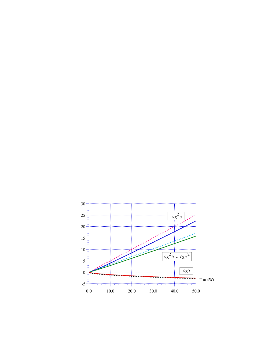
FIG. 1.: Comparison of the two first moments for the reduced one-body probability (left particle) in the lattice (solid lines, eqs. (2.32), (2.34), (2.35)) and continuous framework (dashed lines, eqs. (3.10), (3.12)).

Generally speaking, the transition to continuous isotropic space is achieved from the square lattice framework by setting $W\,=\,D/a^{2}$ and by formally taking the limit $a\rightarrow 0$. Let us set $\phi=k_{1}a$, $\psi=k_{2}a$; when the latter limit is taken, eq. (2.26) generates the Laplace transform of the characteristic function of the two-particle density, $\tilde{f_{\rm L}}(k_{1},k_{2},z)$:

$$\tilde{f_{\rm L}}(k_{1},k_{2},z)\,=\,\frac{1}{\left[z+(D/2)\,(k_{1}+k_{2})^{2}\right]^{1/2}}\,\frac{1}{\left[z+(D/2)\,(k_{1}+k_{2})^{2}\right]^{1/2}\,+\,\rm i\sqrt{D/2}\,(k_{1}-k_{2})}\enspace.$$ (3.1)

This expression is much simpler than its analogous of the discrete version (comp. eq. (2.26)). It can be reexpressed in terms of the total (center-of-mass momentum) $K=k_{1}+k_{2}$ and the relative (reduced) momentum $k=(k_{1}-k_{2})/2$ :

$$\tilde{f_{\rm L}}(k_{1},k_{2},z)\,=\,\frac{1}{\left[z+(D/2)\,K^{2}\right]^{1/2}}\,\frac{1}{\left[z+(D/2)\,K^{2}\right]^{1/2}\,+\,\rm i\sqrt{2D}\,k}\enspace.$$ (3.2)

displaying the fact that the diffusion constant for the center of mass motion is $D/2$, whereas the relative motion has a doubled diffusion constant $2D$ (indeed $D$ plays the same role of an inverse mass in the reduction of a dynamical two-body problem). By using now the Efrös theorem [15], one easily obtains:

$$\tilde{f}(k_{1},k_{2},t)\,=\,{\rm e}^{-DK^{2}t/2}\,\int_{0}^{+\infty}\,\frac{{\rm d}\tau}{\sqrt{\pi\tau}}\,{\rm e}^{-\tau^{2}/(4t)}\,{\rm e}^{-\rm i\sqrt{2D}\,k\tau}\enspace.$$ (3.3)

and Fourier inversion eventually yields the full two-body density probability $P(x_{1},x_{2},t)$ :

$$P(x_{1},x_{2},t)\,=\,\Theta(x_{2}-x_{1})\,\frac{1}{2\pi Dt}\,\mbox{exp}{\left[-\frac{x_{1}^{2}+x_{2}^{2}}{4Dt}\right]}\enspace.$$ (3.4)

where $\Theta(x)$ is the Heaviside unit step function. This expression, obtained as the continuum limit of expression (2.26) is self-evident: provided that the inequality $x_{1}<x_{2}$ is satisfied, each particle has a free diffusion, independently of the other. Obviously, due to the (repulsive) interaction, $P(x_{1},x_{2},t)$ is not the product of two functions, one for each particle. Indeed, $P(x_{1},x_{2},t)$ is an integral of such products:

$$P(x_{1},x_{2},t)\,=\,\lim_{\varepsilon\rightarrow 0}\,\frac{1}{2\rm i\pi^{2}Dt}\,\int_{-\infty}^{+\infty}\,{\rm d}q\,\frac{{\rm e}^{\rm iq(x_{2}-x_{1})}}{q-\rm i\varepsilon}\,{\rm e}^{-(x_{1}^{2}+x_{2}^{2})/(4Dt)}\enspace,$$ (3.5)

exhibiting the obvious fact that the two particles are correlated at all times.

The interparticle correlations are most simply expressed by the correlator $C(t)$, which is readily calculated from eq. (3.4):

$$C(t)\,=\,<(x_{1}-<x_{1}>)\,(x_{2}-<x_{2}>)>\,=\,<x_{1}>^{2}\,=\,\frac{2}{\pi}\,Dt\enspace,$$ (3.6)

showing that the normalized correlator $C(t)/<x_{i}>^{2}$ is constant in time: the correlations induced by the interaction never die out in one dimension.

FIG. 2.: Reduced one-body density for the left particle in the continuous aproximation (see (3.7)). The diffusion constant $D$ is taken as unity and each curve is labelled by the value of time; the asymmetry is less and less pronounced as time increases.

From eq. (3.4), the marginal probabilities in space-time for one particle, obviously asymmetric, are found to be :

$$P_{1,2}(x,t)\,=\,\int_{-\infty}^{+\infty}\,{{\rm d}x^{\prime}}\,P(x,x^{\prime},t)\,=\,\frac{{\rm e}^{-x^{2}/(4Dt)}}{\sqrt{4\pi Dt}}\,\left[1\pm\Phi(x/\sqrt{4Dt})\right]\enspace$$ (3.7)

where the $+$ (resp $-$) sign refers to the right (resp. left) particle and where $\Phi$ denotes the probability integral [16]. The left particle marginal density is plotted in Fig. 2. Setting $k_{2}=0$ (resp. $k_{1}=0$) in eq. (3.3) yields the characteristic functions of the marginal densities:

$$\tilde{f}_{1}(q,t)\,=\,{\rm e}^{-Dq^{2}t/2}\,\int_{0}^{+\infty}\,\frac{{\rm d}\tau}{\sqrt{\pi\tau}}\,{\rm e}^{-\tau^{2}/(4t)}\,{\rm e}^{-{\rm i}\sqrt{D/2}\,q\tau}\enspace,$$ (3.8)

$$\tilde{f}_{2}(q,t)\,=\,[\tilde{f}_{1}(q,t)]^{*}\enspace.$$ (3.9)

These functions give all the moments by successive derivations at $q=0$; thus, at all times:

$$<x_{1}>(t)\,=\,-<x_{2}>(t)\,=\,-\sqrt{\frac{2}{\pi}Dt}\enspace$$ (3.10)

$$<x_{1}^{2}>(t)\,=\,<x_{2}^{2}>(t)\,=\,2Dt\enspace$$ (3.11)

$$\Delta x_{1}^{2}(t)\,=\,\Delta x_{2}^{2}(t)\,=\,2(1-\frac{1}{\pi})\,Dt\enspace$$ (3.12)

These expressions themselves reveal the simplifications carried out by the continuous approximation (comp. (2.32), (2.34) and (2.35)); they also display the expected fact that the exact results at all times of the continuous version coincide with the leading asymptotic terms of the lattice version (see (2.37) and (2.38)); indeed, once the dimensionless time $T=4Wt$ in (2.32) and (2.34) is replaced by $4D/a^{2}$, the limit $a\rightarrow 0$ automatically picks out the first leading term in the asymptotic expansion of the Bessel functions. Note however that lattice effects persist even at very large times: plots given in Fig. 1 allow the comparison between the lattice results (solid curves) and the continuous ones (dashed curves). For the mean square dispersion, the relative “error” decreases slowly as $(Wt)^{-1/2}$: it still amounts to 10% for $Wt=100$. The lattice effects indeed go to zero at infinite times, but in such a slow manner that subdominant terms cannot be neglected on reasonably large times.

On the opposite, with no surprise, the behaviours at short times are markedly different (see (2.39) and Fig.3); for instance, the finite initial drift velocity in the lattice model (see (2.39), which could be observed with high-time resolution experiments, is infinite in the continuous approximation (eq. (3.10)).

Note that the distribution function for the left particle (3.7) satisfies the conservation equation:

$$\frac{\partial P_{1}(x,t)}{\partial t}\,\,=\,-\frac{\partial J(x,t)}{\partial x}\enspace,$$ (3.13)

with:

$$J(x,t)\,=\,-D\,\left[\frac{\partial P_{1}(x,t)}{\partial x}\,+\,2G^{2}_{D}(x,t)\,\right]\enspace,$$ (3.14)

where $G_{D}$ denotes the normal density with a diffusion constant $D$. The additional term to the current is negative for all $x$, as it must clearly be.

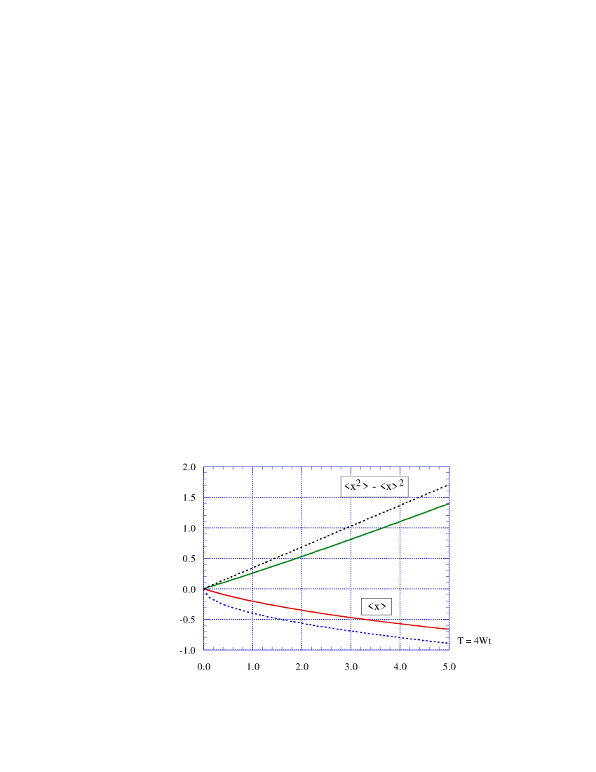
FIG. 3.: Comparison at short times of the two first moments for the reduced one-body probability (left particle) in the lattice (solid lines), and in the continuous framework (dashed lines).

Obviously enough, the results of the continuum approximation are related to the simpler problem of a single fictitious brownian particle in the presence of a perfectly reflecting wall. For the two particles 1 and 2, the diffusion equation writes:

$$\frac{\partial}{\partial t}P(x_{1},x_{2},t)\,=\,D\left(\frac{\partial^{2}}{\partial x_{1}^{2}}+\frac{\partial}{\partial x_{2}^{2}}\right)\,P(x_{1},x_{2},t)\hskip 14.22636pt\forall x_{1}\,\neq\,x_{2}\enspace,$$ (3.15)

the solution here satisfying the initial and boundary conditions $P(x_{1},x_{2},t=0)=\delta(x_{1}+0)\,\delta(x_{2}-0)$, ${P(x_{1},x_{2},t)=0}\hskip 5.69054pt{\forall x_{1}\,\geq\,x_{2}}$. An easy way to solve such an equation is to transform to the center-of-mass frame by setting $\quad x\,=\,x_{2}-x_{1}$, $X\,=\,\frac{1}{2}(x_{1}+x_{2})$, $P(x_{1},x_{2},t)\,=\,\Pi(x,X,t)$; indeed, the diffusion constant $D$ plays the same role as an inverse mass in a mechanical two-body problem. This allows to rewrite the diffusion equation (3.15) as the following :

$$\frac{\partial}{\partial t}\Pi(x,X,t)\,=\,\left(\frac{D}{2}\frac{\partial^{2}}{\partial X^{2}}+2D\frac{\partial}{\partial x^{2}}\right)\,\Pi(x,X,t)\hskip 14.22636pt\forall x\,\neq\,0\enspace.$$ (3.16)

with $\Pi(x,X,t)=0\quad\forall x<0$, $\forall X\in\mbox{\bf R}$.

Equation (3.16) displays the diffusion of the center-of-mass (with a constant $D/2$), decoupled from the diffusion of the relative coordinate (with a constant $2D$) in the presence of a perfectly reflecting barrier at the origin. This means that the problem can be solved in two steps, by considering first the diffusive motion of a single fictitious particle with a doubled diffusion constant and by subsequently adding the effect of the center-of-mass motion. As a whole, the solution of the present problem in its continuous version is given by :

$$P(x_{1},x_{2},t)\,=\,G_{D/2}\left(X=\frac{1}{2}(x_{1}+x_{2}),t\right)\,P_{2D}(x=x_{1}-x_{2},t)\enspace$$ (3.17)

where $G_{D/2}$ is the normalized gaussian function describing the free diffusive motion of the center of mass with the diffusion constant $D/2$, whereas $P_{2D}$ is the solution for the single particle (fictitious) constrained by the reflecting wall. As well known (Gardiner, 1990), if the fictitious particle stands at $x=x_{0}>0$ with probability one at $t=0$, one has:

$$P_{2D}(x,t)\,=\,\Theta(x)\,\int_{0}^{+\infty}\,\frac{2}{\pi}\,dk\,\cos kx_{0}\cos kx\,{\rm e}^{-2Dk^{2}t}\enspace.$$ (3.18)

By taking $x_{0}=0+$, by using (3.17) and by performing all the integrations, one recovers the expression given in (3.4), directly obtained as the limit taken from the lattice version.

Note however that the present problem cannot be considered as a single particle one: the separation of the center-of-mass motion is trivial in the sense that it happens as the consequence of discrete space homogeneity, but this center-of-mass, itself having a diffusive motion (not a purely kinematical one), does participate to the spreading in such a way that correlations are always present; this is the reason why $P(x_{1},x_{2},t)$ does not factor out (see (3.4) and (3.5)) and sustains never-ending correlations, as simply expressed by (3.6). On a deeper level, it is seen that the stochastic motion of each particle is no more Markoffian: the Fourier transforms (3.8), (3.9) are not of the form ${\rm e}^{-A\mid q\mid^{\alpha}}$ and do not satisfy the Bachelier - Smoluchovski - Chapman - Kolmogorov chain equation. The presence of one particle thus strongly alters the nature of the motion of the other.

IV Conclusions

The simple problem of two particles diffusing on a lattice with contact repulsive interaction was fully solved at all times by finding the two-particle characteristic function, from which marginal one-particle densities and moments can be easily derived. At short times, the repulsion induces a linear increase of the position for each particle, associated to a finite velocity, and a linear variation of the second cumulant, with a diffusion constant which is halved for obvious physical reasons. In the final regime, each particle still has an effective anomalous drift, its coordinate growing like $t^{1/2}$, associated to a vanishing velocity. On the other hand, the mean square dispersion asymptotically follows a normal diffusion law; nevertheless, by comparison with its value in the absence of interaction, the diffusion constant is reduced by the non-trivial factor $1-1/\pi$. As a whole, there is a cross-over between two normal diffusion regimes, the diffusion constant varying from $D/2$ at short times to $(1-1/\pi)D$ at large times. Independently of the long-lived subdominant terms, it is seen that each particle does not recover its “free” diffusion constant, even at infinite times. For sure, this is a low-dimensionnality effect.

Taking the limit of continuous space first allows to make explicit connection with the problem of a fictitious particle in the presence of a totally reflecting barrier. Second, by analyzing this limit, it can be seen that marked differences exist between the lattice and the continuous versions. With no surprise, behaviours at short times are very different (the initial drift is finite in the lattice, infinite in the continuum). In addition, due to weakly decreasing subdominant terms, behaviours still substantially differ in both frameworks, even at large times: it can be said that lattice effects persist for physically relevant times, formally vanishing only at infinite times. Thus, when it is a given physical feature, the discreteness of space cannot be ignored.

Figure Captions

1. Comparison of the two first moments for the reduced one-body probability (left particle) in the lattice (solid lines, eqs. (2.32), (2.34), (2.35)) and continuous framework (dashed lines, eqs. (3.10), (3.12)).

2. Reduced one-body density for the left particle in the continuous aproximation (see (3.7)). The diffusion constant $D$ is taken as unity and each curve is labelled by the value of time; the asymmetry is less and less pronounced as time increases.

3. Comparison at short times of the two first moments for the reduced one-body probability (left particle) in the lattice (solid lines), and in the continuous framework (dashed lines).

REFERENCES

• [1] M. E. Fisher, J. Stat. Phys., 34 667–729, 1984
• [2] T. E. Harris, J. Appl. Prob., 2 323, 1965
• [3] K. Mallick, SystΓ¨mes hors d’équilibre: quelques rΓ©sultats exacts (unpublished, 1996)
• [4] B. Derrida and K. Mallick, J. Phys. A, 30 1031–1046, 1997
• [5] T. Sasamoto and M. Wadati, J. Phys. A, 31 6057–6071, 1998
• [6] T. M. Liggett, Interacting Particle Systems (New York: Springer, 1985)
• [7] P. M. Richards, Phys. Rev. B, 16, 1393, 1977
• [8] E. Nener, Science,256 498, 1992
• [9] B. Sackman, Science, 256 503, 1992
• [10] V. Kukla, J. Kornatowski, K. Demuth, I. Girnus, H. Pfeifer, L. V. C. Rees, S. Schunk, K. K. Unger and J. K. KΓ€rger, Science 272 702,1996
• [11] C. RΓΆdenbeck, J. KΓ€rger and K. Hahn, Phys. Rev. E, 57 4382–4397, 1998
• [12] Cl. Aslangul, Europhys. Let., 44 284–289, 1998
• [13] C. W. Gardiner, Handbook of Stochastic Methods for Physics, Chemistry and the Natural Sciences (Berlin: Springer, 1990)
• [14] E. W. Montroll and B. J. West, in Fluctuation Phenomena, ed E W Montroll and J L Lebowitz (Amsterdam: North Holland, 1979)
• [15] M. Lavrentiev and B. Chabat, MΓ©thodes de la thΓ©orie des fonctions d’une variable complexe (Moscow: Mir,1972)
• [16] I. S. Gradshteyn and I. M. Ryzhik, Table of Integrals, Series and Products (New York: Academic Press,1980)