Suppression of Kondo effect in a quantum dot by external irradiation

Abstract

We demonstrate that the external irradiation brings decoherence in the spin states of the quantum dot. This effect cuts off the Kondo anomaly in conductance even at zero temperature. We evaluate the dependence of the DC conductance in the Kondo regime on the power of irradiation, this dependence being determined by the decoherence.

The Kondo effect have drawn recently a considerable attention in connection with the experiments on quantum dots[1, 2, 3]. Due to the Kondo effect, the temperature dependence of the linear conductance across a dot becomes non-monotonous: Upon lowering the temperature, the conductance first drops due to the conventional Coulomb blockade, but below certain temperature starts growing again[1, 2]. The increase of the conductance is associated with the many-body resonance formed at the Fermi energy. This resonance manifests itself as a peak in the differential conductance $G(V)$ at $V=0$ (zero-bias anomaly) [1, 2, 3, 4, 5]. In a magnetic field, the resonant peak in the density of states and therefore the zero-bias peak in $G(V)$ are split in two; the inter-peak spacing is proportional to the Zeeman energy of the localized spin[1, 2, 3, 5]. These results are similar to the effects considered previously in the context of tunneling through junctions carrying Kondo impurities[6].

Quantum dot devices are highly controllable, and can be operated in regimes inaccessible in the conventional magnetic impurity systems, that were used previously for studying the Kondo effect. Kondo anomaly is a manifestation of a quantum-coherent many-body state. Irradiation of a quantum dot with an AC field offers a new, clever way of affecting its dynamics, which enables one to study the Kondo anomaly in essentially non-equilibrium conditions. The anomaly modified by the irradiation can be investigated by the measurements of the DC $I-V$ characteristics.

Despite a considerable amount of work[7, 8, 9, 10, 11], the physical picture of the influence of irradiation on the Kondo conductance still needs clarification. Nordlander et al.[9] have conjectured that the result of irradiation is qualitatively different in two frequency domains of the AC field: At sufficiently high frequency, irradiation may cause ionization of the quantum dot; loss of the localized spin leads to a suppression of the Kondo anomaly in $G(V)$. At frequencies below the ionization threshold, irradiation induces satellite peaks[7, 8, 9, 10] in the differential conductance at $eV=n\hbar\omega$, where $\omega$ is the frequency of the irradiation. The Kondo effect in these conditions, according to [9, 10], is not suppressed. At zero temperature, it is “redistributed” between the usual equilibrium Kondo peak at $eV=0$, and its satellites[10]: The zero-bias conductance departs from the unitary limit, and the satellite peaks appear at its expense; this departure is weak as long as the amplitude of AC modulation of the dot’s energy $eV_{\omega}$ is small.

In this paper we pinpoint the principal effect of the irradiation on the Kondo anomaly. This effect consists in the irradiation-induced decoherence of the localized spin state. Contrary to the picture outlined in the previous paragraph, the decoherence occurs even if the irradiation is not able to ionize the dot. We find the dominant mechanism of decoherence at the frequencies of AC field below the ionization threshold. This mechanism, “spin-flip cotunneling”, leads to a significant deviation of the linear conductance from the unitary limit. Upon the increase of the AC field frequency to the ionization threshold, there is a crossover between the decoherence caused by spin-flip cotunneling and by dot ionization. However, the variation of the conductance in this crossover region is parametrically small. Starting from fairly low frequencies, the suppression of the Kondo conductance by decoherence is more important than the redistribution of the conductance over the high-frequency satellites.

The system we study is a quantum dot attached to two leads by high-resistance junctions so that the charge of the dot is nearly quantized. We describe this system by the Anderson impurity Hamiltonian

$$\hat{H} = \!\sum_{k,\sigma,\alpha}(\xi_{k}+eV_{\alpha})c^{\dagger}_{k\sigma\alpha}c^{\phantom{\dagger}}_{k\sigma\alpha}+\!\sum_{k,\sigma,\alpha}v_{\alpha}(c^{\dagger}_{k\sigma\alpha}d^{\phantom{\dagger}}_{\sigma}+d^{\dagger}_{\sigma}c^{\phantom{\dagger}}_{k\sigma\alpha})$$ (2)

$$+ \sum_{\sigma}(-E_{d}+eV_{\omega}\cos\omega t)d^{\dagger}_{\sigma}d^{\phantom{\dagger}}_{\sigma}+Ud^{\dagger}_{\uparrow}d^{\phantom{\dagger}}_{\uparrow}d^{\dagger}_{\downarrow}d^{\phantom{\dagger}}_{\downarrow}\;;$$ (4)

$$\quad V_{L,R}=\pm\textstyle\frac{1}{2}V\;,\quad\Gamma_{\alpha}\equiv 2\pi\nu v_{\alpha}^{2}\;.$$

Here the first two terms describe non-interacting electrons in the two leads ($\alpha=L,R$), and tunneling of free electrons between the dot and the leads, respectively; we assume tunneling matrix elements $v_{\alpha}$ are real, without reducing the generality of the Hamiltonian. The dot is described by the third and fourth terms of the Hamiltonian, $E_{d}$ and $U-E_{d}$ are the ionization and the electron addition energy, respectively. The tunneling matrix elements $v_{\alpha}$ are related to the widths $\Gamma_{\alpha}$ by Eq. (4), where $\nu$ is the density of states in a lead. The external irradiation is applied to the gate, which is coupled to the dot capacitively, and modulates the energy of the electron localized in the dot. We assume that the leads are DC-biased, neglecting the possible “leakage” of the irradiating AC field to the leads. The generalization onto the case of nonzero AC bias is straightforward.

In the present paper we consider the dot in the Kondo regime, $U-E_{d},\,E_{d}\gg\Gamma_{L,R}$. We assume the applied DC and AC fields are small, $eV,eV_{\omega}\ll E_{d},U-E_{d}$. We are primarily interested in the irradiation effects in the domain $\omega<E_{d},U-E_{d}$, where neither dot ionization nor the photon-assisted tunneling [12] occur. Under such conditions, one can make the Schrieffer-Wolff transformation [13] (more precisely, its modification for the time-dependent case) to convert the Hamiltonian (4) to the Kondo form:

$$\hat{H}_{K} = \hat{H}_{0}+\hat{H}_{t}\;,\quad\hat{H}_{0}=\sum_{k,\sigma,\alpha}\xi_{k}^{\phantom{\dagger}}c^{\dagger}_{k\sigma\alpha}c^{\phantom{\dagger}}_{k\sigma\alpha}\;,$$ (5)

$$\hat{H}_{t} = \!\sum_{\parbox{21.68121pt}{$k,\sigma,\alpha$\\ $k^{\prime}\!,\sigma^{\prime}\!\!,\alpha^{\prime}$}}\!{\cal J}_{\alpha\alpha^{\prime}}(t)\left(\textstyle\frac{1}{4}\delta_{\sigma\sigma^{\prime}}+\hat{S}_{j}s^{j}_{\sigma\sigma^{\prime}}\right)c^{\dagger}_{k\sigma\alpha}c^{\phantom{\dagger}}_{k^{\prime}\sigma^{\prime}\alpha^{\prime}}\;,$$ (6)

where ${\hat{\bf s}}$ and ${\hat{\bf S}}$ are the spin operators of the delocalized electrons in the leads and of the electron on the isolated level, respectively; we assume summation over the repeating indices $j=x,y,z$. The applied bias is accounted for by the time dependence of the coupling term $\hat{H}_{t}$. The Hamiltonian (5) operates within the band $-E_{d}<\xi_{k}<U-E_{d}$, see Ref. [14]. The coupling constants ${\cal J}$ are given by

$${\cal J}_{\alpha\alpha^{\prime}}(t)=\frac{\sqrt{\Gamma_{\alpha}\Gamma_{\alpha^{\prime}}}}{4\pi\nu}\exp\left[\frac{ie}{\hbar}(V_{\alpha}-V_{\alpha^{\prime}})t\right]$$ (7)

$$\times\sum_{n_{1},n_{2}}J_{n_{1}}\left(\frac{eV_{\omega}}{\hbar\omega}\right)J_{n_{2}}\left(\frac{eV_{\omega}}{\hbar\omega}\right)\exp[i(n_{1}-n_{2})\omega t]$$ (8)

$$\times\left[\frac{1}{E_{d}+n_{1}\hbar\omega}+\frac{1}{U-E_{d}+n_{1}\hbar\omega}\right.$$ (9)

$$\left.\;\;\;\;\;\;+\frac{1}{E_{d}+n_{2}\hbar\omega}+\frac{1}{U-E_{d}+n_{2}\hbar\omega}\right]\;,$$ (10)

where $J_{n}(x)$ are the Bessel functions.

To calculate the differential DC conductance $G(V)$, we employ the non-equilibrium Keldysh technique in the time representation. In this formalism

$$G(V)=\frac{\partial}{\partial V}\langle{\sf S}(-\infty,0)\hat{I}{\sf S}(0,-\infty)\rangle_{0}\;,$$ (11)

where $\hat{I}$ is the current operator, and ${\sf S}(t_{2},t_{1})$ is the evolution matrix determined by $\hat{H}_{t}$.

In the perturbation expansion of (11) in powers of the coupling constant ${\cal J}_{\alpha\alpha^{\prime}}$, the logarithmic divergences appear starting from the terms of the third order in ${\cal J}_{\alpha\alpha^{\prime}}$. A representative term has the following structure:

$$\frac{e^{2}}{\pi\hbar}\frac{\left[{\cal J}_{LR}^{\rm(0)}\right]^{2}{\cal J}_{RR}^{\rm(0)}}{\hbar^{3}}\int_{-\infty}^{0}dt_{1}\int^{0}_{t_{1}}dt_{2}\langle\hat{S}_{j}(0)\hat{S}_{k}(t_{1})\hat{S}_{l}(t_{2})\rangle\varepsilon^{jkl}$$ (12)

$$\qquad\times\left[t_{1}\cos(eVt_{1}/\hbar)+t_{2}\cos(eVt_{2}/\hbar)\right]$$ (13)

$$\qquad\times\sum_{k_{1},k_{2},k_{3}}G_{k_{1}}(-t_{2})G_{k_{2}}(t_{2}-t_{1})\bar{G}_{k_{3}}(t_{1})\;,$$ (14)

$$\mbox{where}\quad{\cal J}_{\alpha\alpha^{\prime}}^{\rm(0)}\equiv\frac{\sqrt{\Gamma_{\alpha}\Gamma_{\alpha^{\prime}}}}{\pi\nu\tilde{E}_{d}},\quad\tilde{E}_{d}\equiv\frac{(U-E_{d})E_{d}}{U}\;,$$ (15)

$G_{k}(t)$ and $\bar{G}_{k}(t)$ are the time-ordered and anti-time-ordered Green functions of free electrons in the leads, and $\varepsilon^{jkl}$ is the antisymmetric unit tensor. This and other terms of the same structure yield the Kondo divergency in the conductance. If there is no spin decoherence, the averages $\langle\hat{S}_{j}(t_{1})\hat{S}_{k}(t_{2})\hat{S}_{l}(t_{3})\rangle$ are independent on time and equal $(i/4)\varepsilon_{jkl}$. The AC field introduces decoherence in the dynamics of the impurity spin, which results in a decay of the correlation function:

$$\langle\hat{S}_{j}(t_{1})\hat{S}_{k}(t_{2})\hat{S}_{l}(t_{3})\rangle=(i/4)\varepsilon_{jkl}\exp(-t_{max}/\tau)\;,$$ (16)

$$t_{max}\equiv\max\{|t_{1}-t_{2}|,|t_{2}-t_{3}|,|t_{1}-t_{3}|\}\;.$$ (17)

After summing over the electron states $k_{i}$, performing the integration over $t_{2}$ in Eq. (14), and adding up all the cubic in ${\cal J}^{\rm(0)}$ terms, we arrive at

$$G^{(3)}(V)=12\pi^{2}\frac{e^{2}}{\pi\hbar}\nu^{3}\left[{\cal J}_{LR}^{\rm(0)}\right]^{2}\left[{\cal J}_{RR}^{\rm(0)}+{\cal J}_{LL}^{\rm(0)}\right]$$ (18)

$$\quad\times\int^{0}_{-\infty}\!\!dt\,\frac{(-t)\cos(eVt/\hbar)\exp(-|t|/\tau)}{\sinh^{2}(\pi Tt/\hbar)+(T/D_{0})^{2}}\left(\frac{\pi T}{\hbar}\right)^{2}.$$ (19)

The effective bandwidth here is $D_{0}\equiv\sqrt{E_{d}(U-E_{d})}$ [14]. In the absence of spin decoherence, the integral in Eq. (19) equals $\ln(D_{0}/\max\{T,eV\})$, and diverges logarithmically at low temperature and bias, signaling the Kondo anomaly. The leading effect of the irradiation is in cutting off this divergency. The decay of the spin correlation function (17) makes $G^{(3)}(V)$ finite even at $T,V\to 0$. We will show that the spin decoherence by external irradiation does not require ionization of the impurity level, and therefore exists at arbitrary low frequencies of the applied AC field. The suppressing effect of the irradiation on the Kondo conductance, $G^{(3)}\propto\left[{\cal J}^{\rm(0)}\right]^{3}\ln(D_{0}\tau/\hbar)$, is not analytic in the intensity of the AC field, and cannot be obtained by a finite-order perturbation theory.

In the absence of the dot ionization, the decoherence rate can be calculated with the help of the Hamiltonian (5)–(10). In the case of weak modulation, $eV_{\omega}<\hbar\omega$, it is sufficient to account for the single-photon processes only. The part of Hamiltonian (5)–(10) responsible for such processes corresponds to four terms labeled by $n_{1}=0$, $n_{2}=\pm 1$, and $n_{1}=\pm 1$, $n_{2}=0$ in the sum (10), and is given by

$$\hat{H}_{t}^{(1)}=-\frac{eV_{\omega}\cos\omega t}{2\tilde{E}_{d}}\sum_{\parbox{21.68121pt}{$k,\sigma,\alpha$\\ $k^{\prime}\!,\sigma^{\prime}\!\!,\alpha^{\prime}$}}{\cal J}_{\alpha\alpha^{\prime}}^{\rm(0)}\hat{S}_{j}s^{j}_{\sigma\sigma^{\prime}}c^{\dagger}_{k\sigma\alpha}c^{\phantom{\dagger}}_{k^{\prime}\sigma^{\prime}\alpha^{\prime}}\;.$$ (20)

In deriving Eq. (20), we expanded the Bessel functions of Eq. (10) up to the first order in $eV_{\omega}/\hbar\omega$.

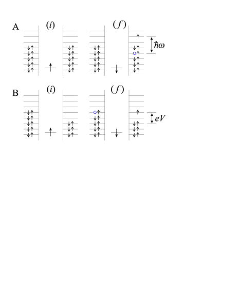
FIG. 1.: Spin-flip cotunneling: the coherence of the spin state of the dot can be lost when an electron interacting with it hops from a state below the Fermi level to a state above the Fermi level. Additional energy, needed for such a transition, can be taken either from the AC field or from the applied bias. The figure shows the initial $(i)$ and final $(f)$ states of the system for the decoherence processes driven by an AC field (A) and by a finite bias (B).

The process of spin-flip cotunneling (spin flip without ionization of the dot) induced by the irradiation is shown schematically in Fig. 1A. In terms of the Kondo Hamiltonian (5), an electron, which interacts with the dot spin, absorbs a photon and hops to a state above the Fermi level, while the spin of the dot flips. Within the lowest-order perturbation theory, the rate of this process can be calculated with the Fermi Golden Rule applied to Hamiltonian (20):

$$\frac{\hbar}{\tau}=\frac{1}{2\pi}\hbar\omega\left[\frac{\Gamma_{L}+\Gamma_{R}}{\tilde{E}_{d}}\right]^{2}\left[\frac{eV_{\omega}}{\tilde{E}_{d}}\right]^{2}\;.$$ (21)

The spin-flip cotunneling persists at arbitrary low frequencies, leading to the decoherence of the dot spin state.

As we pointed out earlier, the Kondo anomaly is a manifestation of a quantum-coherent many-body state. The loss of spin coherence suppresses the Kondo anomaly. At $T,V\to 0$, it is the spin decoherence time $\tau$ what cuts off the logarithmic divergency in the integral (19). After the first logarithmic correction (19) to the conductance is found, we can proceed with the derivation of the Renormalization Group equation, which yields the conductance $G$ in the leading logarithm approximation. For the present non-equilibrium problem, we have to modify the “poor man’s” technique[15] in order to apply it directly to $G$, rather than to the scattering amplitudes. This need emerges from the kinetic nature of the problem at hand. The resulting formula for the peak conductance, which is valid in the domain $\hbar/\tau\gtrsim T_{K}$, can be cast in the form

$$G_{\rm peak}=\frac{e^{2}}{\pi\hbar}\frac{4\Gamma_{L}\Gamma_{R}}{(\Gamma_{L}+\Gamma_{R})^{2}}\frac{3\pi^{2}}{8}\left[\ln\frac{\hbar}{\tau T_{K}}\right]^{-2}.$$ (22)

The width of the conductance peak is $V^{*}\sim\hbar/e\tau$. Here the Kondo temperature $T_{K}$ is defined as [14]

$$T_{K}=\gamma\sqrt{\frac{(\Gamma_{L}+\Gamma_{R})U}{\pi}}\exp\left[-\frac{\pi\tilde{E}_{d}}{2(\Gamma_{L}+\Gamma_{R})}\right]\;,$$ (23)

with $\gamma\sim 1$.

At $\hbar/\tau\gg T_{K}$, one can expand Eq. (22) into the series of powers of $[(\Gamma_{L}+\Gamma_{R})/\tilde{E}_{d}]\ln(D_{0}\tau/\hbar)$. The zero-order term of the series is the conductance calculated in the Born approximation, and the next term yields the lowest order Kondo correction given by Eq. (19). At $\hbar/\tau\lesssim T_{K}$, we expect, in the spirit of the renormalizability of the Kondo problem, that the $(\ln x)^{-2}$ function in Eq. (22) can be replaced by some universal function ${\cal F}(x)$. In the limit of no irradiation, ${\cal F}(0)=8/3\pi^{2}$ (unitary limit of the Kondo scattering).

As the frequency $\omega$ of the AC field grows, the rate of the decoherence processes increases, and the height of the zero bias conductance peak $G_{\rm peak}$ drops. The dependence of $G_{\rm peak}$ on $\omega$ can be found from Eq. (22). For a relatively weak AC field, $eV_{\omega}\ll\tilde{E}_{d}$, the decoherence time $\tau$ is given by Eq. (21) for the frequencies below the ionization threshold $\varepsilon_{i}$, and by $\hbar/\tau=(\Gamma/2)(eV_{\omega}/\tilde{E}_{d})^{2}$ above the threshold. One can easily check that the crossover between these two regimes leads only to parametrically small relative variations in the peak conductance, as $\omega$ increases, say, from $\varepsilon_{i}/2$ to $2\varepsilon_{i}$.

Another effect of external irradiation on the differential conductance $G(V)$ is in producing satellite peaks at $eV=n\hbar\omega$. If an external AC field is applied, then, at $eV=n\hbar\omega$, a tunneling electron can hop from a state at the Fermi level in one lead to a state at the Fermi level in the other lead, emitting or absorbing $n$ photons. Thus at finite bias the external irradiation can effectively put a tunneling electron into zero-bias conditions, and the Kondo anomaly in the conductance is revived. The height of these peaks can be calculated from the formula (11) similarly to Eq. (19). Here we give the results for the first satellite peak. At low enough irradiation level, $eV_{\omega}<\hbar\omega$, it is sufficient to consider only one-photon processes, accounted for by the Hamiltonian (20). The resulting correction to the conductance at $e|V|$ close to $\hbar\omega$ has the form

$$G^{(3)}_{\rm sat}(V)=3\pi^{2}\frac{e^{2}}{\pi\hbar}\nu^{3}\left[{\cal J}_{LR}^{\rm(0)}\right]^{2}\left[{\cal J}_{RR}^{\rm(0)}+{\cal J}_{LL}^{\rm(0)}\right]\left[\frac{eV_{\omega}}{\tilde{E}_{d}}\right]^{2}$$ (24)

$$\times\int^{0}_{-\infty}\!\!dt\,(-t)\exp(-|t|/\tau_{\rm sat})$$ (25)

$$\times\left(\frac{\pi T}{\hbar}\right)^{2}\frac{\cos[(eV/\hbar+\omega)t]+\cos[(eV/\hbar-\omega)t]}{\sinh^{2}(\pi Tt/\hbar)+(T/D_{0})^{2}}\;.$$ (26)

When $eV\neq\pm\,\hbar\omega$, the cosine functions cut off the logarithmic divergences. However, when $eV\to\pm\,\hbar\omega$, one of the two cosine terms becomes essentially constant [cf. Eq. (19) at $V\to 0$], and the differential conductance has a peak again. At $T\to 0$, the height of the conductance peak is determined by the spin decoherence rate $\hbar/\tau_{\rm sat}$. We must mention that $\tau_{\rm sat}$ may be significantly shorter than $\tau$ given by Eq. (21). The time $\tau$ characterizes the spin decoherence at zero bias, whereas the satellite corresponds to a finite bias $eV=\pm\hbar\omega$. In this case, the spin decoherence occurs mostly due to the tunneling of electrons through the dot (see Fig. 1B, and also [5]). The rate of this process is given by

$$\frac{\hbar}{\tau_{\rm sat}}=\frac{1}{2\pi}\,\hbar\omega\,\frac{\Gamma_{L}\Gamma_{R}}{\tilde{E}_{d}^{2}}\;.$$ (27)

Equations (26)–(27) yield the formula for the satellite peak shape, provided $\hbar/\tau_{\rm sat}\gg T_{K}$. The shape of the satellite peak in the conductance is given by

$$G_{\rm sat}(eV-\hbar\omega)=\frac{3}{\pi}\frac{e^{2}}{\pi\hbar}\frac{\Gamma_{L}\Gamma_{R}}{(\Gamma_{L}+\Gamma_{R})^{2}}\left[\frac{eV_{\omega}}{\tilde{E}_{d}}\right]^{2}$$ (28)

$$\times\left[\frac{\Gamma_{L}+\Gamma_{R}}{\tilde{E}_{d}}\right]^{3}\ln\frac{D_{0}}{\sqrt{(\hbar/\tau_{\rm sat})^{2}+(eV-\hbar\omega)^{2}}}\;,$$ (29)

and its width is of the order of $\hbar/e\tau_{\rm sat}$.

At $T\to 0$, i.e., when the unitary limit of tunneling is approached, the formation of the satellite peaks is best viewed as redistribution of the Kondo anomaly between the elastic tunneling processes and the tunneling with absorption/emission of photons[16]. This transfer of spectral weight reduces the height of the zero-bias conductance peak[10]. To compare this mechanism with the spin-flip cotunneling, we note that the redistribution of the Kondo anomaly results from the changes in the single-particle dynamics. To produce a significant deviation of the zero-bias conductance from the unitary limit in this way, one therefore needs to apply an AC field with amplitude

$$V_{\omega}\sim\frac{\tilde{E}_{d}}{e}\;.$$

The spin-flip cotunneling directly affects the many-body state which produces the Kondo anomaly. Due to the fragility of this many-body state, it can be destroyed by a relatively weak AC field; the Kondo effect is suppressed already at

$$\frac{\hbar}{\tau(V_{\omega})}\gtrsim T_{K}\;,$$

with $\tau(V_{\omega})$ given by Eq. (21). Comparing these two conditions on $V_{\omega}$, we find that the decoherence yields the leading effect of AC field on the zero-bias DC conductance starting from parametrically small frequencies, $\hbar\omega>T_{K}(E_{d}/\Gamma)^{2}$ of the AC field.

In conclusion, we have demonstrated that the irradiation suppresses the DC Kondo conductance across a quantum dot. This suppression is an essentially non-perturbative phenomenon. Irradiation brings decoherence into the spin dynamics of the dot, even if the photon energy is insufficient to ionize the dot. Finite lifetime of the Kondo resonance, resulting from the irradiation-induced decoherence, is the main cause of the suppression of the Kondo effect. For suppression to occur, it is sufficient that the spin decoherence time $\tau$, given by Eq. (21), is shorter than characteristic scale $\hbar/T_{K}$ defined by the Kondo temperature $T_{K}$ [Eq. (23)]. The spin decoherence leads to saturation of the low-temperature conductance at $\tau\lesssim\hbar/T$. The condition $\tau\lesssim\hbar/T_{K}$ is readily satisfied at a relatively small amplitude of the AC field, when the redistribution of the differential conductance from the zero-bias peak to the satellite peaks is negligible.

The work at the University of Minnesota was supported by NSF Grant DMR 97-31756. LG acknowledges the hospitality of the Delft University of Technology. LG and AK acknowledge also the hospitality of Institute of Theoretical Physics supported by NSF Grant PHY 94-07194 at University of California at Santa Barbara, where a part of the work was performed. The authors are grateful to L.P. Kouwenhoven, D. Goldhaber-Gordon and Y. Meir for useful discussions.

REFERENCES

- [1] D. Goldhaber-Gordon et al., Nature 391, 156 (1998).
- [2] S.M. Cronenwett, T.H. Oosterkamp, L.P. Kouwenhoven, Science 281, 540 (1998).
- [3] J. Schmid, J. Weis, K. Eberl, K. von Klitzing, Physica B 256–258, 182 (1998).
- [4] S. Hershfield, J.H. Davies, J.W. Wilkins, Phys. Rev. Lett. 67, 3720 (1991).
- [5] Y. Meir, N.S. Wingreen, P.A. Lee, Phys. Rev. Lett. 70, 2601 (1993); N.S. Wingreen, Y. Meir, Phys. Rev. B 49, 11 040 (1994).
- [6] J. Appelbaum, Phys. Rev. Lett. 17, 91 (1966); Phys. Rev. 154, 633 (1967); L.Y.L. Shen, J.M. Rowell, Solid State Commun. 5, 189 (1967); Phys. Rev. 165, 566 (1968).
- [7] M.H. Hettler, H. Schoeller, Phys. Rev. Lett. 74, 4907 (1995).
- [8] T.-K. Ng, Phys. Rev. Lett. 76, 487 (1996).
- [9] P. Nordlander, N.S. Wingreen, Y. Meir, D.C. Langreth, cond-mat/9801241.
- [10] R. López, R. Aguado, G. Platero, C. Tejedor, Phys. Rev. Lett. 81, 4688 (1998).
- [11] Y. Goldin, Y. Avishai, Phys. Rev. Lett. 81, 5394 (1998).
- [12] L.P. Kouwenhoven et al., Phys. Rev. B 50, 2019 (1994); Phys. Rev. Lett. 73, 3443 (1994).
- [13] J.R. Schrieffer, P.A. Wolff, Phys. Rev. 149, 491 (1966).
- [14] F.D.M. Haldane, J. Phys. C 11, 5015 (1978).
- [15] P.W. Anderson, J. Phys. C 3, 2436 (1970).
- [16] P.K. Tien, J.P. Gordon, Phys. Rev. 129, 647 (1963).