Theory of monolayers with boundaries: Exact results and Perturbative analysis

Abstract

Domains and bubbles in tilted phases of Langmuir monolayers contain a class of textures known as boojums. The boundaries of such domains and bubbles may display either cusplike features or indentations. We derive analytic expressions for the textures within domains and surrounding bubbles, and for the shapes of the boundaries of these regions. The derivation is perturbative in the deviation of the bounding curve from a circle. This method is not expected to be accurate when the boundary suffers large distortions, but it does provide important clues with regard to the influence of various energetic terms on the order-parameter texture and the shape of the domain or bubble bounding curve. We also look into the effects of thermal fluctuations, which include a sample-size-dependent effective line tension.

I Introduction

Monolayers of insoluble surfactant molecules confined to the air/water interface possess complex phase structures [1]. In the “tilted” phases, the long axes of the surfactant molecules in the monolayer are uniformly tilted with respect to the normal and the molecular tilt azimuth organizes spontaneously on macroscopic length scales. The structures adopted by the molecular tilt azimuth are referred to as textures. There is no long-range order of the tilt azimuth in the liquid expanded ($LE$) and the gaseous ($G$) phases. Tilted phases can coexist with the $LE$ and $G$ (isotropic) phases and form micron-sized domains. Alternatively, bubbles of an isotropic phase may appear against a background of a tilted phase. Nontrivial textures in the domains, and around the bubbles, have been observed in the $L_{2}/LE$ and $L_{2}/G$ coexistence region, where the $L_{2}$ phase is one of the tilted phases. Boojum textures, similar to those seen in superfluid ³He[2] and smectic-$I$ (Sm-$I$) droplets in liquid-crystal films[3], have been observed in the interior of $L_{2}$ domains [4]. An “inverse boojum,” which is the texture around the bubble analogous to the boojum in the case of the domain, has been identified [5]. The domains and bubbles associated with boojums are not circular. Among the nontrivial domain shapes seen are protrusions on both bubbles and domains, at times sharp enough to be characterized as “cusps”[4, 5] and indentations in domain boundaries which impart a cardioid appearance to the domain [6, 7]. Such domains and bubbles with unusual textures and shapes ought to be observable in other tilted phases as well.

The above textures can be understood in terms of continuum elastic theories of smectic liquid crystals[8]. The bulk energy is controlled by elastic moduli that quantify the energy cost of bend and splay distortions. There are also contributions to the boundary energy, known as the line tension, that depend on the relative angle between the boundary normal and the tilt azimuth. In equilibrium, the texture in a domain or surrounding a bubble, and the shape of the boundary between condensed and expanded regions, adjust so as to minimize the total energy of the monolayer. Domains with nontrivial textures and shapes represent the compromise arising from the competition between the bulk energy and the line tension.

Simultaneous determination of the texture and the boundary of the domain poses a calculational challenge. Earlier studies include the exact result discovered by Rudnick and Bruinsma for a domain with isotropic elastic energy and only the first anisotropic contribution in the Fourier expansion of the line tension $\sigma(\phi)$ [9], and the perturbation about the exact result in terms of coefficient of the second anisotropic term in the expansion[9]. Galatola and Fournier have approached the problem of domains with elasticity and line-tension anisotropies by searching numerically for the equilibrium domain shapes and positions of domains in a fixed texture background [10]. Rivière and Meunier [4] have attributed their experimental findings on domain shapes and textures to elasticity anisotropy in the same manner as in Ref. [10]. In the work of Fang et al. [5], nontrivial boundary shapes for both domains and bubbles, as well as the “inverse boojum” textures in the $L_{2}$ phase surrounding the bubbles, have been reported. A brief account of the theoretical understanding of the bubbles has also been presented in Ref. [5].

In this work, we extend the effort of Rudnick and Bruinsma [9] to analyze the problem of domains with anisotropic elastic energy in addition to the line-tension anisotropy. We also generalize the approach to the problem of bubbles and provide a detailed derivation of the results that have been published in Ref. [5]. Careful analysis reveals that although protrusions can be expected to form on the boundary of a domain of the $L_{2}$ phase, a “cusp” in the form of a discontinuity in the slope of the bounding curve surrounding the domain will not appear in the parameter regime that is appropriate to the analysis that has been carried out [9, 10, 5]. The conclusion in Ref. [9] that a cusp exists is due to an approximation[12] that affects the qualitative results of the analysis. The fact that the cusp does not exist and the condition for the existence of cusps on the boundary were first pointed out by Galatola and Fournier [10]. A formal derivation of the conditions for the appearance of a cusp will be provided in this paper. Perturbative results, which yield the effects of small anisotropies on the textures and boundaries, are obtained. The reliability of the perturbative approach when the boundary is significantly different from a circle is not obvious. Nevertheless, one is provided with useful insights with regard to the influence of various contributions to the energy of the Langmuir monolayer. In addition, we examine the effect of thermal fluctuations. We are led to a renormalized line tension that depends on the radius of the boundary[11].

We have also implemented a numerical program using finite element methods for evaluation of the equilibrium texture and boundary simultaneously. With the use of this approach, we are able to explore regions of the parameter space that are not accessible to the perturbative technique. A brief report on the numerical work has already appeared [13]. A full description of this method and a systematic review of the results of its implementation are deferred to a future article.

The organization of this paper is as follows. In Sec.  II, we describe the approach in general. In Sec. III, we summarize the exact analytic results. Section IV displays the perturbative analysis of the relation between the texture and the boundary. Sections V and VI describe the analysis for the cases of domains and bubbles that results from perturbing about the exact solutions. In Sec. VII, we analyze the effect of thermal fluctuations. Concluding remarks are contained in Sec. VIII.

II The Approach

We describe the monolayer by an ordered phase with $XY$-like order parameter $\hat{c}(x,y)=\hat{x}\cos\Theta(x,y)+\hat{y}\sin\Theta(x,y)$, a two-dimensional unit vector indicating the direction of the projection onto the substrate of the tilted hydrophobic tail of the surfactant forming the Langmuir monolayer. The quantity, $\Theta(x,y)$, is the angle that $\hat{c}(x,y)$ makes with the $x$ axis. When a region $\Omega$ contains an ordered phase which is invariant under in-plane reflection, the free energy of the system takes the general form [8]

$$H[\Theta(x,y)]= \int_{\Omega}{\cal H}_{b}\;dA+\oint_{\Gamma}\sigma[\vartheta-\Theta(x,y)]ds,$$ (1)

where

$${\cal H}_{b}= \frac{K_{s}}{2}|\nabla\cdot\hat{c}(x,y)|^{2}+\frac{K_{b}}{2}|\nabla\times\hat{c}(x,y)|^{2},$$ (2)

$$\sigma(\phi)= \sigma_{0}+\sum_{n=1}a_{n}\cos n\phi.$$ (3)

Here, $K_{s}$ and $K_{b}$ are, respectively, the splay and bend elastic moduli, and $\vartheta$ is the angle between the outward normal of the boundary and the $x$ axis. The quantity $\sigma_{0}>0$ is the isotropic line tension. The first integral is over the area, $\Omega$, of the system, while the second is over the boundary, $\Gamma$, as indicated. The setup of the problem in plane-polar coordinates is shown in Fig. 1.

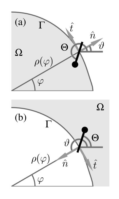
FIG. 1.: The geometry of the calculations for (a) domains and (b) bubbles in plane-polar coordinates where the boundary $\Gamma$ is parametrized by $\rho(\varphi)$. The gray area is the bulk designated by $\Omega$. $\hat{n}$ and $\hat{t}$ are the outward normal and the tangent, respectively. $\Theta$ is the angle between the $\hat{c}$ director and the $x$ axis and $\vartheta$ is the angle between the outward normal of the boundary and the $x$ axis.

Minimization of the energy leads to equations for $\Theta(x,y)$ and the bounding curve $\Gamma$. $\Theta(x,y)$ satisfies

$$-\nabla^{2}\Theta+b\left[\left(\Theta_{xx}-\Theta_{yy}\right)\cos 2\Theta+2\Theta_{xy}\sin 2\Theta\right.$$ (4)

$$\left.+\left(-\Theta_{x}^{2}+\Theta_{y}^{2}\right)\sin 2\Theta+2\Theta_{x}\Theta_{y}\cos 2\Theta\right] =0$$ (5)

in $\Omega$ and

$$\kappa\Theta_{n}\left[1-b\cos 2(\vartheta-\Theta)\right]+$$ (6)

$$\kappa b\Theta_{t}\sin 2(\vartheta-\Theta)-\sigma^{\prime}(\vartheta-\Theta) =0$$ (7)

along $\Gamma$, where $\Theta_{n}=\hat{n}\cdot\nabla\Theta$, $\Theta_{t}=\hat{t}\cdot\nabla\Theta$, $\hat{n}$ and $\hat{t}$ are, respectively, the outward normal and tangential vectors, and

$$\kappa=\frac{K_{s}+K_{b}}{2},$$ (8)

$$b=\frac{K_{s}-K_{b}}{K_{s}+K_{b}}.$$ (9)

The primes attached to functions denote derivatives, e.g., $\sigma^{\prime}(\phi)=d\sigma(\phi)/d\phi$. The extremum equation for the bounding curve $\Gamma$, implicitly in terms of $\Theta_{n}$, $\Theta_{t}$, and $d\vartheta/ds$, is

$${\cal H}_{b}-\sigma^{\prime}(\vartheta-\Theta)\Theta_{n}-\sigma^{\prime\prime}(\vartheta-\Theta)\Theta_{t}$$ (10)

$$+\left[\sigma(\vartheta-\Theta)+\sigma^{\prime\prime}(\vartheta-\Theta)\right]\frac{d\vartheta}{ds}+\lambda =0,$$ (11)

where $ds$ is the length element of $\Gamma$ traversing in the positive direction of $\Omega$ and $\lambda$ is a Lagrange multiplier that enforces the condition of constant enclosed area. The set of equations, Eqs. (5), (7), and (11), are highly nonlinear. It appears, in general, impossible to find general analytical solutions to this set of equations. However, there are full analytical solutions for special cases.

III Exact solutions

We start with the assumption of a circular boundary. We restrict our considerations to isotropic elastic moduli, i.e., $b=0$. Additionally, we assume that the anisotropic line tension, as given by the expansion in Eq. (3), contains only one term, in that $a_{n}=0$ for all $n\neq p$. We will take $a_{p}>0$. This is because the texture with $a_{p}<0$ can be trivially obtained by rotating all $\hat{c}(x,\,y)$ simultaneously by $(2m+1)\pi/p$, where $m$ is an integer $\in$ $[0,p-1]$, due to the symmetry in the line tension. In this special case, Eq. (5) reduces to Laplace’s equation

$$\nabla^{2}\Theta=0,$$ (12)

and Eq. (7) in the plane-polar coordinate system becomes

$$\kappa\Theta_{\rho}-\sigma^{\prime}(\varphi-\Theta) = 0,$$ (13)

$$\kappa\Theta_{\rho}+\sigma^{\prime}(\pi+\varphi-\Theta) = 0,$$ (14)

where Eq.(13) applies to the case of a domain while Eq. (14) is appropriate to the case of a bubble. In two dimensions, the solution to Laplace’s equation can be written in general as

$$\Theta(k,\varphi)=\frac{1}{i}[f(\mbox{e}^{k+i\varphi})-f(\mbox{e}^{k-i\varphi})],$$ (15)

with $f(z)$ an analytic function of $z=\mbox{e}^{k+i\varphi}$ in the region of interest, $\Omega$ for our case. In the case of a circular domain of radius $R_{0}$ centered at the origin, it is shown in Appendix C that

$$\Theta_{0}(k,\varphi) = \frac{1}{i}\left[f_{0}(\mbox{e}^{k+i\varphi})-f_{0}(\mbox{e}^{k-i\varphi})\right],$$ (16)

$$f_{0}(z) = \frac{1}{p}\ln(1-\alpha_{p}z^{p}),$$ (17)

$$\alpha_{p}R_{0}^{p} = -\epsilon+\sqrt{1+\epsilon^{2}},$$ (18)

satisfy Eq. (13). We have defined here a dimensionless parameter $\epsilon=\kappa/(pa_{p}R_{0})$. Figure 2 illustrates such solutions for $p=1,\;2,\;3,\mbox{ and }4$. Also displayed in the figure on the background of each plot is a simulation of the image that would be obtained by Brewster angle microcopy (BAM). The BAM reflectance depends on the exact experimental setup and the properties of the monolayer. A detailed discussion on the computation of the BAM reflectance can be found in Ref. [14]. In the case of all simulated images presented in Fig. 2 and elsewhere in this paper, the Brewster angle is taken to be that of water $\Theta_{B}=53.12^{\circ}$, the angle of the analyzer $\alpha$ is equal to $90^{\circ}$, the thickness of the monolayer is assumed to be $d=0.3\;nm$, the tilt $\Psi$ is $30^{\circ}$, the dielectric constants of the monolayer are $\epsilon_{\perp}=2.31$ and $\epsilon_{\parallel}=2.53$, and it is assumed that the wavelength of the light $\lambda=514\;nm$. Figure 3 shows the order-parameter distribution along the boundary for the solution for $p=1$. The plot of the order-parameter distribution along the boundary is an effective way to examine the texture quantitatively.

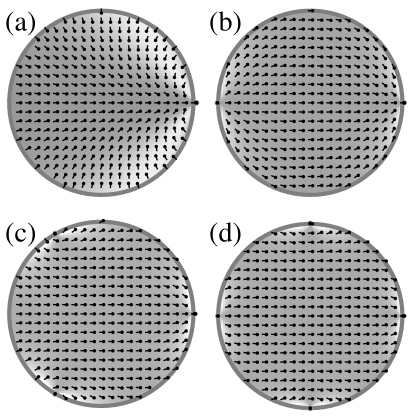
FIG. 2.: The $\hat{c}$ director distribution and the BAM reflectance in a domain computed for $\kappa=1$, $R_{0}=20$, and $a_{p}=1.6$, where $p=1$ in (a), $p=2$ in (b), $p=3$ in (c), and $p=4$ in (d).

When $p=1$, the resulting texture is referred to as the boojum texture. It corresponds to a defect with winding number +2 [15] lying a distance $R_{B}=1/\alpha_{1}$ from the center of the domain. As $\epsilon\rightarrow\infty$, the virtual defect retreats to infinity. As $\epsilon\rightarrow 0$, corresponding to a very strong anisotropic surface energy, or a very large domain, the virtual defect approaches the edge of the domain. However, the distance of the virtual singularity from the boundary of a very large domain remains nonzero, approaching the limit $\kappa/a_{1}$ as $\epsilon\rightarrow\ 0$.

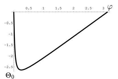
FIG. 3.: The order-parameter distribution along the boundary shown as a plot of $\Theta_{0}$ versus $\varphi$, where $\varphi$ is the polar angle in the plane-polar coordinates. The parameters are $\kappa=1$, $R_{0}=20$, and $a_{1}=1.6$

For the case of a bubble, instead of Eq. (15), we make use of

$$\Theta(k,\varphi)=\frac{1}{i}\left[f\left(\mbox{e}^{-k+i\varphi}\right)-f\left(\mbox{e}^{-k-i\varphi}\right)\right],$$ (19)

as a solution to Laplace’s equation. We find that

$$\Theta_{i}(k,\varphi) = \frac{1}{i}\left[f_{0}\left(\mbox{e}^{-k+i\varphi}\right)-f_{0}\left(\mbox{e}^{-k-i\varphi}\right)\right]+\pi,$$ (20)

$$\frac{\alpha_{p}}{R_{0}^{p}} = -\epsilon+\sqrt{1+\epsilon^{2}},$$ (21)

satisfy Eq. (14) in the case of a circular bubble of radius $R_{0}$ centered at the origin. $\Theta_{i}$ is show in Fig. 4 for $p=1,\;2,\;3,\;\mbox{ and }4$. Also shown in the background of each plot is the intensity distribution that would be recorded in a BAM image.

When $p=1$, $\Theta_{i}$ in Eq. (20) can be characterized as an inverse boojum texture, in that it is obtained by replacing $k$ by $-k$ in $\Theta_{0}$. This corresponds to a defect with winding number $-2$ located at a distance $R_{B}=\alpha_{1}$ from the center of the bubble. When $\epsilon=\infty$, the defect is at the origin. As $\epsilon\rightarrow 0$, it moves towards the edge of the bubble and approaches a distance, $\kappa/a_{1}$, from the boundary.

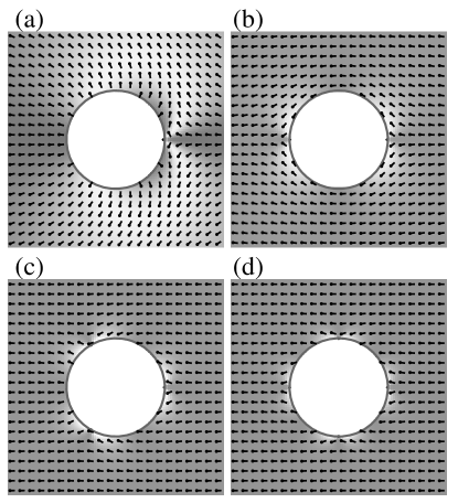
FIG. 4.: The $\hat{c}$ director distribution and the BAM reflectance for bubble computed for $\kappa=1$, $R_{0}=20$, $a_{p}=1.6$, where $p=1$ in (a), $p=2$ in (b), $p=3$ in (c), and $p=4$ in (d).

Note that in the above discussion the domain and the bubble have been assumed to be circular. There is no a priori assurance that this shape minimizes the energy of the system.

As the next step, we determine the equilibrium shape of the domain or bubble. Rewriting $\Gamma$ as $\rho(\varphi)\equiv\mbox{e}^{k(\varphi)}$, that is, in polar coordinates, we transform Eq. (11) into

$$\pm{\cal H}_{b}\mbox{e}^{k}+\left\{-\sigma^{\prime}(\vartheta-\Theta)\Theta_{k}-\sigma^{\prime\prime}(\vartheta-\Theta)\Theta_{\varphi}+\left[\sigma^{\prime}(\vartheta-\Theta)\Theta_{\varphi}-\sigma^{\prime\prime}(\vartheta-\Theta)\Theta_{k}\right]k^{\prime}\right.$$ (22)

$$\left.+\left[\sigma(\vartheta-\Theta)+\sigma^{\prime\prime}(\vartheta-\Theta)\right]\left(1-\frac{k^{\prime\prime}}{1+k^{\prime 2}}\right)\right\}\frac{1}{\sqrt{1+k^{\prime 2}}}+\lambda =0,$$ (23)

where

$$\vartheta=\left\{\begin{array}[]{ll}\varphi-\tan^{-1}k^{\prime}&\mbox{for domains}\\ \pi+\varphi-\tan^{-1}k^{\prime}&\mbox{for bubbles.}\end{array}\right.$$ (26)

In Eq. (23), $+$ applies in the case of a domain while $-$ is appropriate to the case of a bubble. Equation (23) is a nonlinear second-order differential equation, and there is no indication that an analytic solution is possible. However, for the specific case of domain in which $b=0$ and $a_{n\neq 1}=0$ except $a_{1}$, it can be verified that a circular boundary centered at the origin is indeed a solution. Furthermore, such a texture-boundary combination has been shown [16] to be a locally stable configuration. Interestingly, a circular boundary with the inverse boojum texture fails to satisfy Eq. (23) in the case of a bubble.

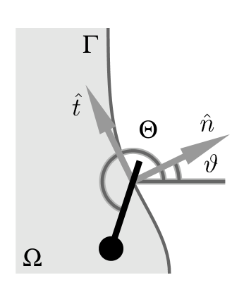
FIG. 5.: The geometry of the calculations for domains and bubbles in Cartesian coordinates. The gray area is the bulk designated by $\Omega$. $\hat{n}$ and $\hat{t}$ are the outward normal and the tangent, respectively. $\Theta$ is the angle made between the $\hat{c}$ director and the $x$ axis and $\vartheta$ is the angle made by the outward normal of the boundary and the $x$ axis.

IV Texture and Boundary Shape

In this section, we assume that the virtual boojum singularity lies close to the boundary between a domain or bubble and the neighboring medium, and we focus on the boundary in the immediate neighborhood of the singularity. This allows us to treat the two regions as semi-infinite. The anisotropic phase is taken to occupy (approximately) the half-space for which $x$ is negative. The setup of the computation is depicted in Fig. 5. We first fix the boundary to lie along the $y$ axis. We then determine the texture in the anisotropic phase when $b=0$ and all the $a_{n}$’s except $a_{1}$ are equal to zero. The order-parameter field $\Theta(x,y)$ will be of the form displayed in Eq. (15), satisfying the boundary condition

$$\left[\kappa\Theta_{x}+a_{1}\sin(-\Theta)\right]_{x=0}=0.$$ (27)

This boundary condition is satisfied by the following expression:

$$\Theta_{C0}(x,y) = \frac{1}{i}[f_{0}(x+iy)-f_{0}(x-iy)],$$ (28)

where $f_{0}(z)$ is as given in Eq. (17) and $\alpha=a_{1}/\kappa$. This texture in fact corresponds to that of a domain in polar coordinates. Inspection of the boundary condition Eq. (27) leads us to another solution $\Theta_{Ci}=-\Theta_{C0}$, which corresponds to the texture of a bubble in cylindrical geometry. Figures 6(a) and 6(b) show the distributions of the order parameter and the computed BAM image in this geometry for the domain and the bubble, respectively. The correspondence between $\Theta_{C0}$ and $\Theta_{0}$ for the case of domains can be observed in Fig. 6(a) in that the $\hat{c}$ directors tend to point towards each other around the $x$ axis. Figure 6(b) corresponds to Fig. 4(a) for the case of bubbles in that the $\hat{c}$ directors fan out in the direction of the outward normal of the boundary near the $x$ axis.

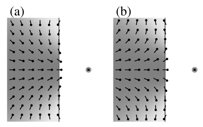
FIG. 6.: The order-parameter distribution and the BAM reflectance when the boundary $\Gamma$ is a straight line for $\kappa=1$ and $a_{1}=1.6$, where (a) shows $\Theta_{C0}$ for the case of a domain while (b) shows $\Theta_{Ci}$ for the case of a bubble.

To investigate the equilibrium condition for the boundary $\Gamma$, we parametrize $\Gamma$ in Cartesian coordinates by $x=\eta(y)$. The equilibrium condition for $\Gamma$ can then be written as

$$\frac{\kappa}{2}\left|\nabla\Theta\right|^{2}+\sigma^{\prime}(\vartheta-\Theta)\frac{\eta^{\prime}\Theta_{y}-\Theta_{x}}{\sqrt{1+\eta^{\prime 2}}}+\frac{d\vartheta}{d\eta^{\prime}}\sigma^{\prime\prime}(\vartheta-\Theta)\left(\Theta_{y}+\eta^{\prime}\Theta_{x}\right)\sqrt{1+\eta^{\prime 2}}$$ (29)

$$-\left[\sigma(\vartheta-\Theta)+\sigma^{\prime\prime}(\vartheta-\Theta)\right]\frac{\eta^{\prime\prime}}{\sqrt{1+\eta^{\prime 2}}^{3}}+\lambda =0,$$ (30)

and for the boundary condition at $y=0$

$$\eta^{\prime}=\frac{d\vartheta}{d\eta^{\prime}}\left(1+\eta^{\prime 2}\right)\frac{\sigma^{\prime}(\vartheta)}{\sigma(\vartheta)},$$ (31)

where $\vartheta=-\tan^{-1}\eta^{\prime}$ is the angle between the outward normal $\hat{n}$ of $\Gamma$ and the $x$ axis.

A cusplike singularity occurs when $\eta^{\prime}(0)\neq 0$. As a result of the symmetry of the problem, $\eta(-y)=\eta(y)$ and $\eta^{\prime}(-y)=-\eta^{\prime}(y)$. The possible values of $\eta^{\prime}(0)$ can be obtained by solving Eq. (31). That $\eta^{\prime}(0)=0$ is a solution follows from the fact that $\sigma^{\prime}(0)=0$. In order that a nonzero $\eta^{\prime}(0)$ solves Eq. (31), the slope of the right-hand side of Eq. (31) at the origin must be greater than unity, or

$$\frac{d}{d\eta^{\prime}}\left[\frac{d\vartheta}{d\eta^{\prime}}(1+\eta^{\prime 2})\frac{\sigma^{\prime}(\vartheta)}{\sigma(\vartheta)}\right]_{\eta^{\prime}=0}\geq 1,$$ (32)

which leads us to the cusp condition $\sigma(0)\;[\sigma(0)+\sigma^{\prime\prime}(0)]\leq 0$. We will exclude such a condition from our discussion, as it requires either $|a_{1}|\geq\sigma_{0}$ or $3a_{2}\geq\sigma_{0}$. Such conditions are incompatible with the parameter regime on which we focus.

It can be shown that $x=0$ or the $y$ axis is a solution to Eq. (30) when $\Theta_{C0}$ is used as the texture (for the case of domain) while this is not so for the case of the bubble, or when the texture is $\Theta_{Ci}$. We continue to investigate perturbatively the response to the texture when the boundary deviates slightly from $x=0$. Let the texture, $\Theta(x,y)$, be of the form of Eq. (15) with

$$f(z)\approx f_{0}(z)+\xi(z)f^{\prime}_{0}(z).$$ (33)

Both $\eta(y)$, the deviation of the boundary from the straight line $x=0$, and $\xi(z)$ in Eq. (33) are small quantities. They possess the following properties:

$$\eta(x)=\eta(-x)$$ (34)

$$\xi(z)=\xi^{*}(z^{*})$$ (35)

The boundary condition can then be expressed as

$$\left.\kappa\left(\frac{\partial}{\partial x}+\eta\frac{\partial^{2}}{\partial x^{2}}-\vartheta\frac{\partial}{\partial y}\right)\Theta\right|_{x=0}+$$ (36)

$$\left.\rule{0.0pt}{14.45377pt}a_{1}\sin(\vartheta-\Theta)\right|_{x=\eta} \approx 0,$$ (37)

where $\vartheta\approx-\eta^{\prime}$. To first order in $\eta,\xi$ and their derivatives, we obtain the following equations:

$$\frac{2\alpha y\xi^{\prime}(iy)}{1+\alpha^{2}y^{2}}=-\frac{2\alpha^{2}y\eta(y)}{1+\alpha^{2}y^{2}}\pm\vartheta,$$ (38)

where $+$ corresponds to the case of domain and $-$ corresponds to the case of bubble. The relation between $\eta$ and $\xi$ is readily derived:

$$\xi(iy)=\int^{iy}_{0}\frac{1+\alpha^{2}y^{\prime 2}}{2\alpha y^{\prime}}\left[-\frac{2\alpha^{2}y^{\prime}\eta(y^{\prime})}{1+\alpha^{2}y^{\prime 2}}\pm\vartheta\right]dy^{\prime}.$$ (39)

Here, we distinguish the primes attached to functions which denote derivatives and those attached to variables within the integrals which indicate that they are variables of integration. Primes will be used in this fashion from now on. The function $\xi$ obtained from Eq. (39) is defined along the $y$ axis. We now analytically continue $\xi$ to the entire $x-y$ plane. Up to this point, we have expressed the distortion of the texture in terms of a fixed boundary deviation from the exact solution given in the beginning of the section. To examine the solution Eq. (39), it is necessary to determine the textural deformation associated with $\eta(y)=\eta_{0}$ for domain. We find

$$\xi(z)=-\alpha\eta_{0}z.$$ (40)

The resulting texture

$$\Theta(x,y) \approx \frac{1}{i}[f_{0}(x-\eta_{0}+iy)-f_{0}(x-\eta_{0}-iy)]$$ (41)

is identical to the domain texture given in Eq. (28) except that the position of the virtual defect is translated by an amount $\eta_{0}$ in the positive $x$ direction.

Under a small boundary distortion, $x=\eta(y)$ away from the $y$ axis, the function $f(z)$ given in Eq. (33) and its derivative are approximated as

$$f(\eta+iy) = \ln(1-i\alpha y)-\frac{\alpha\xi(iy)}{1-i\alpha y},$$ (42)

$$f^{\prime}(\eta+iy) = -\frac{\alpha}{1-i\alpha y}-\frac{\alpha\xi^{\prime}(iy)}{1-i\alpha y}-$$ (44)

$$\qquad\frac{\alpha^{2}\left[\eta+\xi(iy)\right]}{(1+i\alpha y)^{2}},$$

where $\xi(iy)$ is given in Eq. (38). When these expressions are substituted into Eq. (30) we obtain, for $\Theta=\Theta_{C0}$, which corresponds to the case of domain,

$$\eta^{\prime\prime}=\frac{2\delta\alpha}{1+\alpha^{2}y^{2}}\left[\alpha\eta+\xi^{\prime}(iy)\right],$$ (45)

while, for $\Theta=\Theta_{Ci}$, which corresponds to the case of bubbles,

$$\eta^{\prime\prime}= \delta\left[\frac{4\alpha\left(1-\alpha^{2}y^{2}\right)}{\left(1+\alpha^{2}y^{2}\right)^{2}}+\frac{2\alpha^{2}\left(3-10\alpha^{2}y^{2}+3\alpha^{2}y^{4}\right)}{\left(1+\alpha^{2}y^{2}\right)^{3}}\eta+\frac{8i\alpha^{3}y\left(3-\alpha^{2}y^{2}\right)}{\left(1+\alpha^{2}y^{2}\right)^{3}}\xi(iy)+\frac{2\alpha\left(3-\alpha^{2}y^{2}\right)}{\left(1+\alpha^{2}y^{2}\right)^{2}}\xi^{\prime}(iy)\right],$$ (46)

where $\delta\equiv a_{1}/\sigma_{0}$. We can see that the right-hand side of the equation for the distorting effect of the texture appropriate to a domain, i.e., Eq. (45), starts at first order in $\eta$ while the corresponding equation, Eq. (46), for a bubble starts at zeroth order in $\eta$. This provides further confirmation that there is no simple inversion symmetry between the domain and bubble.

V Domains

We have established that the boojum texture together with a circular boundary is an exact solution for the case in which $b=0$ and only $a_{1}\neq 0$. This leads us to the conclusion that nonzero $b$ and/or higher harmonics in the expansion Eq. (3) must be present if the boundary is to be noncircular. We now attempt to analyze the situation in which $a_{1}$, $a_{2}$, and $b$ are all nonzero. We do this by perturbing about the boojum solution in terms of small parameters $b$ and $\gamma$, where $\gamma\equiv a_{2}/a_{1}$.

We note here that the sign of $a_{1}$ does not affect any of the following analysis. As has been mentioned in Sec. II, if $\Theta_{0}$ is an equilibrium texture for $a_{1}>0$, then $\Theta=\Theta_{0}+\pi$, representing a reflection of the $\hat{c}$ directors about the $x$ axis, will be the corresponding texture for $a_{1}<0$. The equilibrium boundary is circular in both cases. Furthermore, contributions of $b$ and $a_{2}$ appear in the form of $\Theta_{z}\mbox{e}^{i2\Theta}$, which is invariant under reflection of the $\hat{c}$ directors about the $x$ axis. $\Theta_{z}$ represents derivatives of $\Theta$ with respect to the variable $z$ which can be $x$, $y$, or any linear combination of the two. Hence, the effect of $a_{2}$ and $b$ is independent of the sign of $a_{1}$. In the upcoming discussions, we will assume $a_{1}>0$ for convenience. The inequality $\gamma>0$ refers to the case in which the $\hat{c}$ directors along the boundary prefer to lie tangent to it while $\gamma<0$ applies when the $\hat{c}$ directors prefer to point along the normal to the boundary, $\pm\hat{n}$. When $b>0$, bend textures are preferred; splay is preferred when $b<0$.

We first find the textural response to $\gamma$ and $b$ by making use of Eq. (15) with

$$f(z)=f_{0}(z)+f_{1}(z).$$ (47)

It can be shown that Eq. (5) is satisfied even with $f_{1}(z)=0$. We continue to investigate the boundary condition of the texture assuming that the bounding curve is a circle of radius $R_{0}$. Equation (7) requires a nonzero $f_{1}(z)$ satisfying

$$\kappa[zf_{1}^{\prime}(z)-z^{-1}f_{1}^{\prime}(z^{*})]+\frac{a_{1}}{2}\left[\left(-\frac{z-\alpha}{1-\alpha z}-\frac{1-\alpha z}{z-\alpha}\right)f_{1}(z)+\left(\frac{z-\alpha}{1-\alpha z}+\frac{1-\alpha z}{z-\alpha}\right)f_{1}(z^{*})\right]$$ (48)

$$+\frac{\kappa b\alpha}{R_{0}}\left[\frac{1-\alpha z}{z(1-\alpha z^{*})^{2}}-\frac{z(1-\alpha z^{*})}{(1-\alpha z)^{2}}\right]+a_{2}\left[\left(\frac{z-\alpha}{1-\alpha z}\right)^{2}-\left(\frac{1-\alpha z}{z-\alpha}\right)^{2}\right] =0.$$ (49)

In contrast to the notation used in Eqs. (17) and (18), we have redefined $z\equiv\mbox{e}^{i\varphi}$ and absorbed $R_{0}$ into $\alpha\equiv R_{0}\alpha_{1}$. Equation (49) can be separated into two equations:

$$zf^{\prime}_{1}(z)-\frac{1}{2\epsilon}\left(\frac{z-\alpha}{1-\alpha z}+\frac{1-\alpha z}{z-\alpha}\right)f_{1}(z)=b\alpha\frac{z-\alpha}{z(1-\alpha z)^{2}}-\frac{\gamma}{\epsilon}\left(\frac{z-\alpha}{1-\alpha z}\right)^{2}$$ (50)

and an identical equation with $z$ replaced by its complex conjugate $z^{*}$. Each of these equations is solvable by standard methods. One finds

$$f_{1}(z) = \frac{\gamma}{\alpha(\alpha+\epsilon)}\frac{z-\alpha}{1-\alpha z}-\frac{\epsilon(b\alpha-2\gamma)}{\alpha+\epsilon}\frac{(z-\alpha)}{1-\alpha z}\;\/_{2}F_{1}(1,\alpha/\epsilon+1;\alpha/\epsilon+2;-\alpha z),$$ (51)

where ${}_{2}F_{1}(\nu,\mu;\mu+1;z)$ is a hypergeometric function[17]. With $f_{1}(z)$ included, $\Theta(x,y)$ now satisfies Eq. (5) up to first order in $\gamma$ and $b$.

The full analytical solution of Eq. (23) is difficult when $\gamma$ and $b$ are both nonzero. However, one can attempt a solution as an expansion in the small parameters $\gamma$, $b$, $k$, and $k^{\prime}$. We recall the definition of $\rho(\varphi)\equiv\mbox{e}^{k(\varphi)}\approx 1+k(\varphi)$. If one ignores terms beyond first order in these quantities, it is possible to solve for the bounding curve, $\Gamma$, analytically. The algebraic manipulations are dramatically simplified if we further approximate $\Theta_{n}\approx\Theta_{k}/R_{0}$ and $\Theta_{t}\approx\Theta_{\varphi}/R_{0}$, which is equivalent to neglecting the first-order contributions of $k^{\prime}(\varphi)$. The error of the analysis is then of order $\sim O(\delta k^{\prime})$, where $\delta\equiv a_{1}/\sigma_{0}$, which has been defined earlier in Sec. IV. The equation for the boundary $\Gamma$,

$${\cal H}_{b}R_{0}+\left\{-\sigma^{\prime}(\varphi-\Theta)\Theta_{k}-\sigma^{\prime\prime}(\varphi-\Theta)\Theta_{\varphi}\right.$$ (52)

$$\left.+\left[\sigma(\varphi-\Theta)+\sigma^{\prime\prime}(\varphi-\Theta)\right]\left(1-k^{\prime\prime}\right)\right\}+\lambda =0,$$ (53)

can then be reduced to

$$k^{\prime\prime}(\varphi)=k_{1}^{\prime\prime}(\varphi)+k_{2}^{\prime\prime}(\varphi)+k_{3}^{\prime\prime}(\varphi),$$ (54)

where $k^{\prime\prime}$ has been separated into various components, as shown below, for convenience,

$$k_{1}^{\prime\prime}(\varphi) = \frac{\delta b\alpha^{2}(-z+\alpha+\epsilon)}{(1-\alpha z)^{2}}+\mbox{c.c.},$$ (55)

$$k_{2}^{\prime\prime}(\varphi) = -\delta\alpha\gamma\left(\frac{z}{1-\alpha z}+\frac{3}{z-\alpha}+\frac{3}{2\alpha}-\frac{1}{\epsilon z}\right)\left(\frac{z-\alpha}{1-\alpha z}\right)^{2}+\mbox{c.c.},$$ (56)

$$k_{3}^{\prime\prime}(\varphi) = \delta\alpha\left[\frac{1}{1-\alpha z}-\frac{z}{z-\alpha}-\frac{1}{2\epsilon z}\left(\frac{z-\alpha}{1-\alpha z}+\frac{1-\alpha z}{z-\alpha}\right)\right]f_{1}(z)+\mbox{c.c.}$$ (57)

$k_{1}(\varphi)$ consists of terms that depend on $b$, $k_{2}(\varphi)$ contains terms that depend on $\gamma$, and $k_{3}(\varphi)$ has terms that depend on both $b$ and $\gamma$ through the textural correction $f_{1}$ given in Eq.  (51). The functions $k^{\prime}(\varphi)$ and $k(\varphi)$ can then be obtained by integrating Eq. (54) with respect to $\varphi$. They are

$$k_{1}^{\prime}(\varphi) = \frac{\delta b\alpha^{2}}{i}\left[-(\epsilon+\alpha)\ln(1-\alpha z)+\frac{1-\alpha^{2}-\alpha\epsilon}{\alpha(\alpha z-1)}\right]-\mbox{c.c.},$$ (58)

$$k_{2}^{\prime}(\varphi) = -\frac{\delta\alpha\gamma}{i}\left\{\left[\frac{1}{2\alpha}+\frac{3\alpha^{2}}{2}-\frac{1-\alpha^{4}}{\epsilon}\right]\ln(1-\alpha z)+\right.$$ (60)

$$\left.\left[\frac{1}{2\alpha}-\frac{3\alpha}{2}+\frac{1-\alpha^{2}}{\epsilon}\right]\frac{1-\alpha^{2}}{\alpha z-1}+\frac{\left(1-\alpha^{2}\right)^{2}}{2\alpha(\alpha z-1)^{2}}\right\}-\mbox{c.c.},$$

$$k_{3}^{\prime}(\varphi) = -\frac{\delta\alpha}{i\epsilon}\left(b\alpha-\frac{2\gamma}{\delta}\right)g(\alpha z)-\mbox{c.c.},$$ (61)

where

$$g(z) = -\frac{\epsilon}{\alpha+\epsilon}\int^{z}\frac{{}_{2}F_{1}\left(1,\alpha/\epsilon+1;\alpha/\epsilon+2;-z^{\prime}\right)}{z^{\prime}}dz^{\prime}.$$ (62)

One more integration yields

$$k_{1}(\varphi) = \delta b\alpha^{2}\left[\left(\epsilon-\frac{1}{\alpha}+\alpha\right)\ln(1-\alpha z)-(\epsilon+\alpha)\mbox{Li}_{2}(\alpha z)\right]+\mbox{c.c.},$$ (63)

$$k_{2}(\varphi) = \frac{\delta\gamma}{\alpha}\left\{-\left[\frac{2}{\alpha}+\frac{3\alpha^{3}}{2}-\frac{1-\alpha^{4}}{\epsilon}\right]\mbox{Li}_{2}(\alpha z)\right.+$$ (65)

$$\left.\left[-\alpha(1-\alpha^{2})+\frac{\left(1-\alpha^{2}\right)^{2}}{\epsilon}\right]\ln(1-\alpha z)-\frac{\left(1-\alpha^{2}\right)^{2}}{2\alpha(\alpha z-1)}\right\}+\mbox{c.c.},$$

$$k_{3}(\varphi) = -\frac{\delta\alpha}{\epsilon}\left(b\alpha-\frac{2\gamma}{\delta}\right)h(\alpha z)+\mbox{c.c.},$$ (66)

where

$$h(z)=\int^{z}g(z^{\prime})/z^{\prime}dz^{\prime}$$ (67)

and Li${}_{2}(z)$ is the polylogarithmic function defined as

$$\mbox{Li}_{n}(x) =\sum_{k=1}^{\infty}\frac{x^{k}}{k^{n}}.$$ (68)

Numerical integrations can be utilized for the evaluation of $k(\varphi)$. However, as we can see from the following,

$$\int^{z}_{0}\frac{z^{\prime\alpha/\epsilon}}{1-\alpha z^{\prime}}dz^{\prime}=-\frac{\epsilon z^{\alpha/\epsilon+1}}{\alpha+\epsilon}\/_{2}F_{1}(1,\alpha/\epsilon+1;\alpha/\epsilon+2;-\alpha z),$$ (69)

the integrand oscillates strongly as $\alpha/\epsilon\rightarrow\infty$ as a result of the factor $z^{\prime\alpha/\epsilon}$ and numerical integrations become inefficient. Further observation reveals that $g(z)$ and $h(z)$ can be evaluated analytically if $\alpha/\epsilon\equiv n$ is an integer. Equation (69) simplifies as follows:

$$\int^{z}_{0}\frac{z^{\prime n}}{1-\alpha z^{\prime}}dz^{\prime}=-\alpha^{-n-1}\left[\sum^{n}_{i=1}\frac{(\alpha z)^{i}}{i}+\ln(1-\alpha z)\right].$$ (70)

When the above simplification is substituted into Eq. (62), the integration can be performed and yields the analytic form of $g(z)$:

$$g(z)= \sum_{k=1}^{n}\left[-\frac{1}{n-k+1}+\frac{1}{n+1}\right]\frac{1}{kz^{k}}+\frac{\ln(1-z)}{n+1}\left[1-\frac{1}{z^{n+1}}\right].$$ (71)

$h(z)$ can be evaluated analytically in the same manner and we get

$$h(z)= \sum_{k=1}^{n}\frac{1}{(n-k+1)k^{2}z^{k}}-\sum_{k=1}^{n}\left[\frac{1}{(n+1)^{2}k}+\frac{1}{(n+1)k^{2}}\right]\frac{1}{z^{k}}$$ (73)

$$+\frac{\ln(1-z)}{(n+1)^{2}z^{n+1}}-\frac{\ln(1-z)}{(n+1)^{2}}-\frac{\mbox{Li}_{2}(z)}{n+1}.$$

The boundary of the domain $\displaystyle{k(\varphi)=\sum_{j=1}^{3}k_{j}(\varphi)}$ is smooth and has continuous derivatives. Typical $k(\varphi)$, $k^{\prime}(\varphi)$, and $k^{\prime\prime}(\varphi)$’s are shown in Fig. 7(a). The corresponding boundary $\Gamma$ parametrized by $\rho(\varphi)=1+k(\varphi)$ is depicted in Fig. 7(b). We have thus arrived at an approximate expression for $\Gamma$ as a function of the line-tension anisotropy coefficient $\gamma$ and the elastic anisotropy coefficient $b$. This expression is useful when we are interested in the response of $\Gamma$ for small values of the these anisotropic parameters.

We first examine the boundary response to $\gamma$ while keeping $b=0$. We find indentations and protruding features on the domain boundary for $\gamma<0$ and $\gamma>0$, respectively. The progressive change of the boundary response when $a_{2}$ changes from $-0.5$ to $0.5$ is illustrated in Fig. 8. The results are in qualitative agreement with those presented in Ref. [10]. We have also examined the dependence of the boundary at fixed $\gamma$ on domain size, $R_{0}$. Figure 9 show boundaries for domains of sizes $R_{0}=0.2$ to $10$. When $R_{0}<1$, the domains appear slightly flattened and elongated if $\gamma>0$. This is in accord with the intuitive notion that the second-harmonic term in the line tension becomes important as the variation in the texture vanishes, i.e., in the limit that the order parameter is uniform. As the domain gets larger, the boojum singularity moves closer to the edge of the domain and the boundary correction moves towards the axis connecting the center of the domain and the boojum. Cusplike features start to appear when the domain is larger than a “threshold” size, $R_{0}=1$ for the domains in Fig. 9. We note that we have used large values of $\gamma\leq 0.3$ to illustrate the nontrivial boundary that we have obtained for the domains. It has been numerically verified [13] that the qualitative behavior of the boundary response is indeed preserved up to much larger values of $\gamma$.

It has been shown in Sec. IV that the boundaries of the domains are strictly smooth and continuous in the parameter regime upon which we focus. We are, however, able to find domains with cusplike features in the context of the perturbative analysis described in this paper. Such domains can be characterized by an excluded angle $\Psi_{0}$ defined in Fig. 10(a). Domains with boundaries that resemble those with cusplike features are observed experimentally. The domain-size dependence of $\Psi_{0}$ is shown in Fig. 10(b) [5]. There is no rigorous mathematical definition of $\Psi_{0}$ for a continuous boundary. It is, nevertheless, possible to devise a systematic way of identifying such an excluded angle for a smooth boundary. One first evaluates $\Psi\equiv-2\tan^{-1}dx/dy$ along the boundary. The value of $\Psi$ at the straightest part of the boundary, which is indicated by $d^{2}x/dy^{2}\rightarrow 0$, is a likely candidate for $\Psi_{0}$. Figures 11(a) and 11(b) show the plot of $\Psi$ and $d^{2}x/dy^{2}$ versus $\varphi$, respectively. The values of $\Psi$ in the plateau region in Fig. 11(a) represent the range in which the measured excluded angles are likely to fall. These values of $\Psi$ are found in the region near the $\Psi$ axis of the plot of $\Psi$ versus $d^{2}x/dy^{2}$ shown in Fig. 11(c). A plot of $\Psi$ versus $I\equiv I_{0}\exp[-(d^{2}x/dy^{2})^{2}]$, as shown in Fig. 11(d), highlights the range of the values of $\Psi$ that is most likely to contain the measured excluded angle. Figure 11(e) displays $I$ as the intensity (inverted, in that the brightest corresponds to the smallest value of I). Figure 11(f) shows the value of $\Psi$ at which $I=I_{\mbox{max}}$ by the dark line and the region in which $I>I_{\mbox{max}}/2$, or the full-width-at-half-maximum (FWHM), by the gray band. Figures 11(e) and 11(f) are useful for describing the selection process by which one is led to the most likely values of the excluded angle. Figures 12(a) and 12(b) illustrate such plots. The experimental result is superposed in Fig. 12(b). The parameters are adjusted in order to obtain a by-eye fit. The values of the parameters are $\kappa/a_{1}=4\;\mu$m, $\delta=0.4$, and $\gamma=0.5$

The perturbative analysis generates results that are in good agreement with experimental observations [5] for large domains. It has also captured qualitatively the essential features, namely the onset and the maximum of the domain size dependence of the excluded angle. As displayed in Fig. 12(b), the maximum and the onset of $\Psi_{0}$ are quantitatively different in the perturbative analysis and in the experimental data in the intermediate $R_{0}$ regime. In particular, the experimental maximum of $\Psi_{0}$ cannot be obtained from the analysis even though $\gamma=0.5$ has been used. We shall defer the discussion on this to the end of this section after elaborating on the effect of the elastic anisotropy $b$. We also note that $\gamma=0.5$ is very large as a perturbative parameter. Although there is no a priori guarantee of the accuracy of the results, it is evident from our numerical studies[13] that the qualitative behavior of the boundary as a function of the domain size is preserved in the perturbative analysis up to at least $\gamma=0.5$.

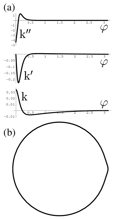
FIG. 7.: (a) Plot of $k^{\prime\prime}(\varphi)$, $k^{\prime}(\varphi)$, and $k(\varphi)$ for $\kappa=1$, $R_{0}=5$, $\sigma_{0}=4$, $a_{1}=1.6$, and $a_{2}$=0.5. (b) The corresponding domain shape $\Gamma$ parametrized as $\rho(\varphi)\approx 1+k(\varphi)$.

We now proceed to examine the effect of $b$ on the boundary $\Gamma$. The coefficient of the anisotropic line tension $\gamma$ is kept at zero and the boundary response is proportional to $b$. Figure 13 shows the plot of $k(\varphi)/b$. In contrast to the results obtained by Galatola and Fournier[10], the boundary acquires a denting correction when $b<0$, indicated by a maximum in $k(\varphi)/b$ at $\varphi=0$. This perturbative result is confirmed for small values of $b$ (=0.1) by our numerical studies [18]. At such small values of $b$, the boundary is practically circular. We shall restrict our discussion to the effect on $\Gamma$ of small values of $b$, in that higher-order corrections of $b$, which are not taken into account in this first-order perturbative analysis, change the qualitative behavior of the boundary response, as reflected by our numerical studies [13].

FIG. 8.: Domain shapes computed for $\kappa=1$, $R_{0}=5$, $\sigma_{0}=4$, $a_{1}=1.6$. and (a) $a_{2}=-0.5$, (b) $a_{2}=-0.3$, (c) $a_{2}=-0.1$, (d) $a_{2}=0.1$, (e) $a_{2}=0.3$, and (f) $a_{2}=0.5$.

FIG. 9.: Domain shapes computed for $\kappa=1$, $\sigma_{0}=4$, $a_{1}=1.6$, $a_{2}=0.6$, and (a) $R_{0}=0.2,0.25,0.33,0.5,1$ and (b) $R_{0}=2,2.5,3.3,5,10$.

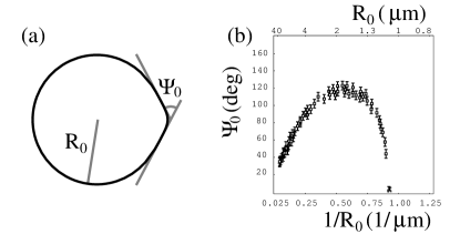
FIG. 10.: (a) The definition of the excluded angle $\Psi_{0}$. (b) Experimental measurements of the domain-size dependence of $\Psi_{0}$ observed in $L_{2}$ domains surrounded by LE phase taken from Ref. [5].

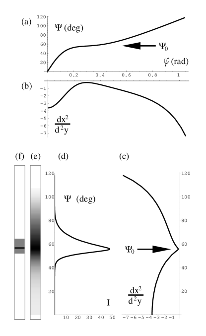
FIG. 11.: (a) Plot of $\Psi\equiv-2\tan^{-1}dx/dy$ versus $\varphi$ for $\kappa=1$, $R_{0}=5$, $\sigma_{0}=4$, $a_{1}=1.6$, and $a_{2}=0.6$. (b) Plot of $d^{2}x/dy^{2}$ versus $\varphi$ for the same parameter. (c) Plot of $\Psi$ versus $d^{2}x/dy^{2}$. (d) Plot of $\Psi$ versus $I\equiv\mbox{exp}[-(d^{2}x/dy^{2})^{2}]$. (e) Density plot of $I$ as $\Psi$ for a single $R_{0}$. (f) The dark line marks the maximum $I_{\mbox{max}}$ of $I$ while the gray region shows the range of $\Psi$ in which $I>I_{\mbox{max}}/2$.

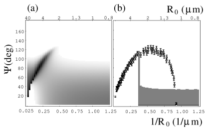
FIG. 12.: (a) Density plot of $I$ as a function of $\Psi$ and $R_{0}$. (b) Plot of $I_{\mbox{max}}$ and the region in which $I>I_{\mbox{max}}/2$ as a function of $\Psi$ and $R_{0}$. Superimposed are the experimental data shown in Fig. 10(b) with parameters $\kappa/a_{1}=4\;\mu$m, $\delta=0.4$, and $\gamma=0.5$.

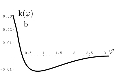
FIG. 13.: Plot of $k(\varphi)/b$ for $\kappa=1$, $R_{0}=5$, $\sigma_{0}=4$, $a_{1}=1.6$, and $a_{2}=0$. The maximum of $k(\varphi)$ at $\varphi=0$ implies a protruding correction when $b>0$.

As for the role of $b$ in the interpretation of the experimental observations, we conclude in our numerical studies [13] that a nonzero value of $b$ cannot be solely responsible for the protruding features, and hence the excluded-angle measurements. Large values of $\gamma\approx 0.5$ are required to produce excluded angles whose maximum approaches the largest value of experimentally measured excluded angles. At sufficiently large values of $\gamma$, we have found that the behavior of the excluded angle is qualitatively unchanged when the anisotropy parameter $b$ is varied from $-0.5$ to 0.5. Although the validity of the perturbative analysis at $b>0.1$ is questionable, the relative magnitude of the correction to the boundary of $b$ is much smaller than that of $\gamma$. This is further verified by numerical studies[18].

We have thus demonstrated, within our first-order perturbative analysis, that the line-tension anisotropy $\gamma$ can give rise to the indentations and protruding features of the domain boundaries that have been experimentally observed [7]. Our results on the boundary response to $\gamma$ are in qualitative agreement with prior results[10, 13]. Although our investigation of the $b$ dependence of the boundary does not provide us with dependable results for large values of $b$, it supports the assertion that the textural correction is an important contribution to the boundary response. Further analysis of the available experimental data on the excluded angles leads to the conclusion that $b$ has little effect on the boundary of the domains with protrusions. We shall confine our conclusions to small values of $|b|<0.1$, although large values of $b\sim 0.8$ do lead to interesting domain shapes. Discussions of the domain boundaries at large values of $b$ will be presented in a forthcoming article [18], and some of the results have been briefly presented in Ref. [13].

We obtain good agreement between the results of the perturbative analysis and the experimental observations on the $\Psi_{0}$ dependence on the domain radius $R_{0}$ in the large-$R_{0}$ regime. In the intermediate-$R_{0}$ regime, the discrepancy is not resolved, even in our numerical studies [18]. The mismatch could possibly be attributed to the fact that our simple elastic theory does not describe accurately the actual complex monolayer. In the perturbative analysis performed in this work, the parameters are restricted to a region in which $\sigma(\varphi)+\sigma^{\prime\prime}(\varphi)$ is always greater than zero. Furthermore, it is generally known that the dipolar interactions between the surfactant molecules in the monolayer are important. The current model does not take into account such interactions. It has been discovered in a recent experimental study [19] that the tilt is not always uniform, especially in the region around a point defect. The contribution of variation in tilt may not be significant in terms of accounting for the discrepancy in the intermediate-sized domain regime. It does become important in the large-$R_{0}$ regime when the virtual singularity approaches the domain boundary and the texture acquires a rapid variation in the neighborhood of the virtual singularity.

VI Bubbles

It has been shown in Secs. III and  IV that there is no straightforward inversion symmetry between the domains and the bubbles. In contrast to the case of the domain, it is not necessary to introduce anisotropic parameters other than $a_{1}$. The inverse boojum texture $\Theta_{i}$ given in Eq. (20) and Eq. (21) satisfies the equilibrium condition for a circular bubble for the case in which the $\hat{c}$ directors favor pointing into the bulk or $a_{1}>0$. Substituting $\Theta_{i}$ into the equilibrium condition for the boundary $\Gamma$ Eq. (23), one finds that a circular boundary does not satisfy the equation. By perturbing about the circular boundary in terms of a small parameter $\delta\equiv a_{1}/\sigma_{0}$, we arrive at an equation similar to Eq. (54),

$$k^{\prime\prime}(\varphi) = -2\alpha^{2}\delta\epsilon\frac{z^{2}}{(1-\alpha z)^{2}}+\mbox{c.c.}$$ (74)

Again—see Eqs (20) and (21)—we have redefined $z\equiv\mbox{e}^{i\varphi}$ and $\alpha\equiv\alpha_{1}/R_{0}$. Following the same procedure as for the case of a domain, we find for $k^{\prime}(\varphi)$ and $k(\varphi)$

$$k^{\prime}(\varphi) = -\frac{2\delta\epsilon}{i}\left[\frac{1}{1-\alpha z}+\ln(1-\alpha z)\right]-\mbox{c.c.},$$ (75)

$$k(\varphi) = -2\delta\epsilon\left[\ln(1-\alpha z)+\mbox{Li}_{2}(\alpha z)\right]+\mbox{c.c.}$$ (76)

It should be kept in mind that the above discussion refers to the case $a_{1}>0$. The results for $a_{1}<0$ are not obtained by a simple sign reversal of $a_{1}$ in Eq. (76). Appropriate changes in the texture and definition of $\epsilon$, which is given as $\kappa/(|a_{1}|R_{0})$, must be taken into account. The details of the calculations are presented in Appendix C. The final bounding curve for the bubble depends only on the magnitude $|a_{1}|$. We have derived expressions for $\Gamma$ for the cases where there is only an $a_{1}$ contribution in the line tension.

FIG. 14.: Bubble shapes computed for $\kappa=0.16$, $\sigma_{0}=1$, $a_{1}=0.16$, and (a) $R_{0}=1,2,3,4,5,6,8$ and (b) $R_{0}=8,20,40$.

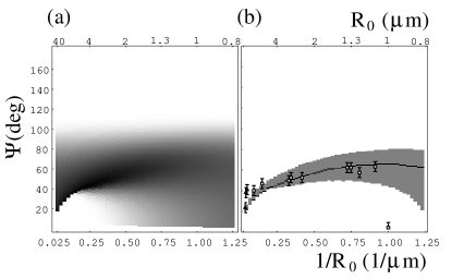
FIG. 15.: (a) Plot of $I$ as a function of $\Psi$ and $R_{0}$. (b) Plot of $I_{\mbox{max}}$ and the region in which $I>I_{\mbox{max}}/2$ as a function of $\Psi$ and $R_{0}$. Superimposed are the experimental observations of gaseous bubbles in $L_{2}$ phase. The experimental data have appeared in Ref. [5]. The parameters for the by-eye fit are $\kappa/a_{1}=0.4\;\mu$m and $\delta=0.16.$

One can utilize the results to investigate the bubble-size dependence of the boundary shapes. Figure 14 shows the shapes for the bubbles of sizes $R_{0}=0.2$ to $10$. Very small bubbles $R_{0}\ll 1$ are nearly circular, as are very small domains. Cusplike features start to appear when the bubble is larger than a “threshold” size, $R_{0}=1$ for the bubbles shown in Fig. 14. Similar analysis of the excluded angle to that for the domain presented in Sec. V can be carried out. Figure 15 shows plots of $\Psi$ versus $R_{0}$ corresponding to those in Fig. 12. Experimental measurements [5] of the cusp angle for the bubble are superposed in Fig. 15(b). A by-eye fit can be obtained with parameters $\kappa/a_{1}=0.4\;\mu$m and $\delta=0.16$. We find fairly reasonable agreement between the theory and experimental observations. We remark that the apparent mismatch between the theory and the experimental data point at $R_{0}=1\;\mu$m, which has been shown to match the explicit measurement on the calculated bubble boundary in Ref. [5], may be the result of the inadequacy in qualifying the excluded angle $\Psi_{0}$ for bubbles with $R_{0}<1\;\mu$m using the FWHM of $I$ shown in Fig. 11(f).

As compared to the parameters obtained for the domains in Sec. V, which are $\kappa/a_{1}=4\;\mu$m, $\delta=0.4$, and $\gamma=0.5$, the value of $\kappa/a_{1}$ for the case of bubbles is an order of magnitude smaller than that for the case of domains. Noting the fact that the data for the bubbles are obtained at the $L_{2}/G$ coexistence region and those of the domains are measured when the $L_{2}$ domains are surrounded by the $LE$ phase [5], the comparison of $\kappa/a_{1}$ between the domains and the bubbles is indeed in accord with the intuitive sense that $\kappa$ of the $L_{2}$ domains should not vary significantly while $a_{1}$ at the $L_{2}/G$ interface is much larger than that at the $L_{2}/LE$ boundary. The $\delta$’s are of the same order of magnitude and there is no corresponding $\gamma$ in the case of bubbles. The result of the perturbative analysis is consistent between the domains and the bubbles.

VII Thermal Fluctuations

The analysis presented in the earlier sections is in the mean-field approximation; thermal fluctuations are ignored. In this section, we examine the effect of thermal fluctuations and its implications to the computation that has been carried out. The effect of fluctuations can be assessed by utilizing a mapping between the statistical mechanics of the order-parameter fluctuations in this system and the behavior of a two-dimensional Coulomb gas[20]. Consider the Hamiltonian of the form of Eq. (1), with $b=0$ and $a_{n}=0$ for all $n\neq p$. For a system with circular boundary of radius $R_{0}$, one has

$$H^{\prime}[\Theta]= H[\Theta]-2\pi\sigma_{0}R_{0}.$$ (77)

the prime here distinguishes the free energy from the one defined in Eq. (1). The prime is dropped from now on for convenience. The partition function can be written as

$$Z(a_{p}) = Z(0)\left\langle\exp\left[-\beta a_{p}\oint\cos p(\varphi-\Theta)ds\right]\right\rangle_{0},$$ (78)

where $\langle{\cal O}\rangle_{0}$ denotes the thermal average with respect to the Hamiltonian without the boundary term given below,

$$\langle{\cal O}\rangle_{0}=\frac{\int{\cal D}\Theta{\cal O}\exp(-\frac{\beta\kappa}{2}\int dA|\nabla\Theta|^{2})}{\int{\cal D}\Theta\exp(-\frac{\beta\kappa}{2}\int dA|\nabla\Theta|^{2})}.$$ (79)

We denote $\Theta_{b}(\varphi)\equiv\Theta(R_{0}\cos\varphi,R_{0}\sin\varphi)$ as the values of $\Theta$ on the boundary of the circular domain. The following correlation function can be evaluated[11],

$$\langle\Theta_{b}(\varphi)\Theta_{b}(\varphi^{\prime})\rangle_{0} = -\Delta\ln 2\left|\sin\frac{\varphi-\varphi^{\prime}}{2}\right|,$$ (80)

where $\Delta\equiv 1/2\pi\beta\kappa$.

To evaluate the full partition function Eq. (78), we Taylor expand the exponent as

$$\frac{Z(a_{p})}{Z(0)}=\sum_{n=0}^{\infty}\left(-\beta a_{p}\right)^{n}\frac{1}{n!}\left\langle\prod_{i=1}^{n}\left[\oint\frac{ds_{i}}{a}\cos p(\varphi_{i}-\Theta_{i})\right]\right\rangle_{0},$$ (81)

where we have added an index $i$ to distinguish the various cosine terms, denoted $\Theta_{i}\equiv\Theta(R_{0}\cos\varphi_{i},R_{0}\sin\varphi_{i})$ for convenience, and introduced a microscopic length scale $a$ in the denominator in $ds$ to make the total integration dimensionless. We use $\cos\phi=\left(\mbox{e}^{i\phi}+\mbox{e}^{-i\phi}\right)/2$ and then expand the products of the cosine terms,

$$\frac{Z(a_{p})}{Z(0)} = \sum_{n=0}^{\infty}\left(\frac{-\beta a_{p}}{2}\right)^{n}\frac{1}{n!}\prod_{i=1}^{n}\oint\frac{ds_{i}}{a}\sum_{\left\{q_{i}\right\}}\left[\mbox{e}^{-i\sum_{i=0}^{n}q_{i}\varphi_{i}}\left\langle\mbox{e}^{i\sum_{i=0}^{n}q_{i}\Theta_{i}}\right\rangle_{0}\right],$$ (82)

where we have defined charge $q_{i}=\pm p$ for each of the cosine terms in Eq. (81) and denoted $\displaystyle{\sum_{\{q_{i}\}}}$ a sum over all charge configurations. The thermal average can be evaluated exactly using Wick’s theorem; we obtain the following equality:

$$\left\langle\mbox{e}^{i\sum_{i=0}^{n}q_{i}\Theta_{i}}\right\rangle_{0}=\mbox{e}^{-\frac{1}{2}\left\langle\left(\sum_{i=0}^{n}q_{i}\Theta_{i}\right)^{2}\right\rangle_{0}}.$$ (83)

The average $\langle\Theta^{2}\rangle_{0}$ encountered in Eq. (83) can be evaluated using the inverse of the microscopic length scale $1/a$ as the ultraviolet cutoff. We have the following:

$$\langle\Theta^{2}(\varphi)\rangle_{0} = \lim_{\varphi\rightarrow\varphi^{\prime}}\langle\Theta(\varphi)\Theta(\varphi^{\prime})\rangle_{0}.$$ (84)

$$= \Delta\ln\frac{R_{0}}{a}.$$ (85)

The contributions of the charge configurations in which $\sum_{i}q_{i}\neq 0$ to the partition function are suppressed as a result of excess factors of $\displaystyle{\exp\left(-\frac{p^{2}\Delta}{2}\ln\frac{R_{0}}{a}\right)}$. Therefore, it is necessary to sum only over the configurations in which there is no net charge. Finally, the full partition function can be expressed as follows:

$$\frac{Z(a_{p})}{Z(0)} = \sum_{n=0}^{\infty}\left(\frac{-\beta a_{p}}{2}\right)^{2n}\frac{1}{(2n)!}\prod_{i=1}^{2n}\oint\frac{ds_{i}}{a}\sum_{\left\{\sum q_{i}=0\right\}}\mbox{e}^{-i\sum_{i=0}^{2n}q_{i}\varphi_{i}}\mbox{e}^{-\frac{\Delta}{2}\sum_{i,j}q_{i}q_{j}\ln\frac{\vec{x}_{i}-\vec{x}_{j}}{a}},$$ (86)

analogous to the expression of the partition function for a system of 2D neutral coulomb gas. The charge of the particles is $p\sqrt{\Delta/2}$ and the particles are distributed along the circumference of the domain. Following the Coulomb gas treatment for the 2D phase transitions[21], we derive flow equations for the running coupling constants,

$$a\frac{da_{p}(a)}{da} = \left[1-\frac{p^{2}\Delta(a)}{2}\right]a_{p}(a),$$ (87)

$$a\frac{d\Delta(a)}{da} = -2\pi^{2}\Delta^{2}(a)a_{p}^{2}(a).$$ (88)

For $a_{p}(a)\ll 1$, we have the following:

$$\frac{a_{p}(a)}{a_{p}(a_{0})}=\left(\frac{a}{a_{0}}\right)^{1-p^{2}\Delta/2}.$$ (89)

The scaling relation implies the relevancy, and the irrelevancy transition temperature of $a_{p}(a)$ at $T_{p}$ is given by

$$k_{B}T_{p}=\frac{4\pi\kappa}{p^{2}}.$$ (90)

As compared to the Kosterlitz-Thouless transition temperature $k_{B}T_{KT}=\pi\kappa/2$, $T_{1}$ and $T_{2}$ are above $T_{KT}$. Our result is analogous to the scaling index of the symmetry-breaking perturbation in the 2D planar model obtained by the spin-wave approximation [22].

In the low-temperature phase, we consider fluctuations up to a cutoff that is proportional to the sample size, or $a\sim R_{0}$, and consider the renormalized coupling constant $a_{p}=a_{p}(R_{0})R_{0}$. We find the scaling relation,

$$a_{p} \sim R_{0}^{-p^{2}\Delta/2}.$$ (91)

Based on a theory of fixed $\kappa$, the renormalized anisotropic line tension decreases as a power law with $R_{0}$, the radius of the boundary, with exponent $-p^{2}\Delta/2$. Using this relation, we investigated the effect of thermal fluctuation on the domain boundary. The result is depicted in plot of $\Psi$ at the maximum of $I$, $\Psi_{0}$, as a function of $R_{0}$ in Fig. 16. We notice the rounding off at the maximum of $\Psi_{0}$ and the decrease in the magnitude of $\Psi_{0}$ with increasing temperature. The above comparisons are made for domains with $\delta=0.4$ and $\gamma=0.38$ when $R_{0}=0.2$.

We can also look at the effect of fluctuations on $b$. We let $a_{n}=0$ for all $n$ and the Hamiltonian becomes

$$H[\Theta]=\frac{\kappa}{2}\int\left\{|\nabla\Theta|^{2}+b\left[\left(-\Theta_{x}^{2}+\Theta_{y}^{2}\right)\cos 2\Theta-2\Theta_{x}\Theta_{y}\sin 2\Theta\right]\right\}dA.$$ (92)

The partition function

$$Z(b)=Z(0)\left\langle\exp\left[\frac{\beta b\kappa}{4}\int\left(\Theta_{{\bar{z}}}^{2}\mbox{e}^{i2\Theta}+\Theta_{z}^{2}\mbox{e}^{-i2\Theta}\right)dA\right]\right\rangle_{0},$$ (93)

which leads to the flow equations similar to those for $a_{k}$,

$$a\frac{db(a)}{da} = -2\Delta(a)b(a),$$ (94)

$$a\frac{d\Delta(a)}{da} = -2\pi^{2}\Delta^{2}(a)b^{2}(a),$$ (95)

from which we deduce that $b$ is always irrelevant at finite temperature.

Following the same argument as for the case of $a_{p}$, we consider fluctuations that cut off at $a\sim R_{0}$ in the ordered phase, and take the renormalized coupling constant $b=b(R_{0})$. We find that the $b$ scales as $R_{0}^{-2\Delta}$ in a theory with fixed $\kappa$. When thermal fluctuations are important, the magnitude $|b|$ is at its maximun ($\leq 1$) for the smallest $R_{0}$ and decreases as $R_{0}$ increases. Thermal effects reduce the already insignificant boundary correction due to $b$. This reinforces our earlier conclusion that $b$ has no significant influence on the domain boundary.

FIG. 16.: Plots of $\Psi_{0}$ as a function of $R_{0}$ for $\kappa=1$, $\sigma_{0}=4$ at $T=0$, $0.1T_{KT}$, $0.3T_{KT}$, $0.5T_{KT}$, and $0.7T_{KT}$. At $R_{0}=0.2$, all domains have the same renormalized coefficients in the expansion of the anisotropic line tension, namely $a_{1}=1.6$ and $a_{2}=0.6$.

In summary, thermal fluctuations act to renormalize the anisotropic parameters. The influence of thermal fluctuations on the boundary shape can be studied using the mean-field approximation with renormalized anisotropic parameters. The boundary correction due to elastic anisotropy, which is negligible at $T=0$, further decreases as a result of thermal fluctuations. The deviation of the boundary from a circle that results from line-tension anisotropy is displayed in terms of the domain-size dependence of the excluded angle in Fig. 10. The maximum of the excluded angle, which is higher in the experimental observations than predicted at $T=0$ (see Fig. 12), will be reduced when thermal fluctuations are introduced. This indicates that the line-tension anisotropy of the monolayer system under study may be very strong.

VIII Conclusions

We have described in this paper a systematic investigation of a system of a 2D ordered medium with a boundary. Beginning with the free energy Eq. (1), which describes a bounded monolayer, we have derived the Euler-Lagrange equations for the texture and the boundary. From the boundary conditions we have shown that the boundary under consideration must be smooth. A continuation of the analysis in the spirit of Ref. [9] for the cases of both the domains and the bubbles reveals that bubbles do not remain circular when the only term in the anisotropic line tension, as given by Eq. (3), is $a_{1}\cos\phi$, while circular domains are not affected. There is, thus, no simple inversion symmetry between domains and bubbles, as one would intuitively expect. Perturbative calculations have been carried out to investigate the influence of the $a_{2}$ term, the second-harmonic contribution in the line tension, and the elastic anisotropy, parametrized by $b$, for the domains. Assuming the domains are nearly circular and the anisotropies are weak, the perturbed domain shapes are then computed analytically to first order in small parameters. We have examined the boundary response to the anisotropic parameters $b$ and $a_{2}$. Our results for the boundary response to $a_{2}$ are in qualitative agreement with those reported in Refs. [10, 13]. We have also obtained the dependence of the boundary shape on domain size that is in qualitative agreement with experimental findings when $b=0$ [5, 7]. As for the boundary response to $b$, our perturbative results contrast with the conclusions arrived at in Ref. [10]. Textural correction plays an important role. These conclusions are confirmed in our numerical studies [13, 18]. The $b$ contribution to the boundary is much weaker than that of the line-tension anisotropy. The quality of the fit to the currently available experimental observations is not sensitive to the value of $b$ in the range from $-0.5$ to $0.5$. Considering only the line-tension anisotropy $a_{2}$, the result of the perturbative analysis has qualitatively captured the essential features of the experimental observations. The quantitative mismatch can be attributed in part to the inapplicability of a perturbative approach to a parameter region in which the anisotropic parameters are large. The detailed difference between the simple model we adopt and the actual complex underlying structure of the $L_{2}$ domains may also contribute to such discrepancies. Long-range dipolar repulsion has been ignored. The tilt degree of freedom  [19], which may not be significant in the small domain regime but can be important in the large-$R_{0}$ region, is not included.

In the case of the bubbles, we evaluate the boundary response due to the $a_{1}$ contribution in the line tension. We are able to produce a dependence of the shape of the bounding curve on bubble size that compares favorably with experimental observations. This result has been reported earlier in Ref. [5]. The parameters of the domains and those of the bubbles, both obtained with by-eye fit of the result of the analysis to the experimental data, are in reasonable agreement, taking into consideration the fact that the data for the domains are taken in the $L_{2}/LE$ coexistence region and those for the bubbles is obtained for gaseous bubbles surrounded by the $L_{2}$ phase. Finally, we have presented an analysis of the effect of thermal fluctuations that leads to a domain-size dependence of the line-tension and elastic anisotropies. The analysis also suggests that the line-tension anisotropy may be very strong.

A Geometry and coordinate systems

We enumerate in this section the forms taken by various geometrical quantities of a 2D space curve in different coordinate systems and the relationships between those forms. A curve $\Gamma$ surrounding $\Omega$ can be represented by a one-parameter trajectory of the position vector $\vec{r}(t)$, where $t$ is parameter. Its unit tangent vector is given by $\hat{t}=d\vec{r}/ds$ and the unit outward normal is given by $\hat{n}=\vec{n}/|\vec{n}|$, where $\vec{n}=\pm d^{2}\vec{r}/ds^{2}$ and $ds\equiv|d\vec{r}/dt|dt$. We let $\vartheta$ be the angle between the normal vector of the curve and a reference axis. Then the radius of curvature is $|ds/d\vartheta|$.

Consider the problem of a nearly circular domain. The coordinate system of choice is obviously plane-polar. It is convenient to use $\varphi$ as the independent variable. We then write $\Gamma$ as $\vec{r}(\varphi)=\mbox{e}^{k(\varphi)}\hat{\rho}$, where $\mbox{e}^{k(\varphi)}$ is the radial distance from the origin and $\varphi$ is the polar angle at $\vec{r}$. A length element given by $ds=\mbox{e}^{k}\sqrt{1+k^{\prime 2}}d\varphi$ is in the positive direction of $\Omega$. The unit vector $\vec{n}=-d^{2}\vec{r}/ds^{2}$ points away from the origin, or outwards from $\Gamma$,

$$\hat{t}= \frac{k^{\prime}\hat{\rho}+\hat{\varphi}}{\sqrt{1+k^{\prime 2}}},$$ (A1)

$$\hat{n}= \frac{\hat{\rho}-k^{\prime}\hat{\varphi}}{\sqrt{1+k^{\prime 2}}}.$$ (A2)

We have $\cos\vartheta=\hat{n}\cdot\hat{x}$, which gives $\vartheta=\varphi-\tan^{-1}k^{\prime}$. It follows that

$$\frac{d\vartheta}{ds}=\left(1-\frac{k^{\prime\prime}}{1+k^{\prime 2}}\right)\frac{1}{\mbox{e}^{k}\sqrt{1+k^{\prime 2}}}.$$ (A3)

Similar relations can be derived for the case of a nearly circular bubble. Here, the length element in the positive direction of $\Omega$ is $ds=-\mbox{e}^{k}\sqrt{1+k^{\prime 2}}d\varphi$ and the outward normal $\vec{n}=d^{2}\vec{r}/ds^{2}$. We obtain $\vartheta=\pi+\varphi-\tan^{-1}k^{\prime}$. The geometrical quantities are evaluated as follows:

$$\hat{t}= -\frac{k^{\prime}\hat{\rho}+\hat{\varphi}}{\sqrt{1+k^{\prime 2}}},$$ (A4)

$$\hat{n}= -\frac{\hat{\rho}-k^{\prime}\hat{\varphi}}{\sqrt{1+k^{\prime 2}}},$$ (A5)

$$\frac{d\vartheta}{ds}= -\left(1-\frac{k^{\prime\prime}}{1+k^{\prime 2}}\right)\frac{1}{\mbox{e}^{k}\sqrt{1+k^{\prime 2}}}.$$ (A6)

Cartesian coordinates are useful when we are interested in a small region of a large circular domain or bubble, on the scale of which the boundary is nearly a straight line. In Cartesian coordinates, we have for the position vector $\vec{r}(t)\equiv x(t)\hat{x}+y(t)\hat{y}$, where $\hat{x}$ and $\hat{y}$ are the unit basis vectors. We can always pick $y$ as the independent variable and $x=\eta(y)$ as the dependent variable for the curve $\Gamma$. The symbol $\eta(y)$ is chosen deliberately to avoid confusion with the independent variable $x$ for the texture $\Theta$. We take $\Omega$ to reside in the region $x<0$, assume that $\Gamma$ nearly coincides with the $y$ axis, and take the virtual defect to be in $x>0$ near the $y$ axis as depicted in Fig. 5. We have $ds=\sqrt{1+\eta^{\prime 2}}dy$ traversing along the positive direction of $\Gamma$ and $\vec{n}=-d^{2}\vec{r}/ds^{2}$. We immediately obtain

$$\hat{t}= \frac{\eta^{\prime}\hat{x}+\hat{y}}{\sqrt{1+\eta^{\prime 2}}},$$ (A7)

$$\hat{n}= \frac{\hat{x}-\eta^{\prime}\hat{y}}{\sqrt{1+\eta^{\prime 2}}}.$$ (A8)

The angle between the normal and the $x$ axis is $\vartheta=-\tan^{-1}\eta^{\prime}$, and

$$\frac{d\vartheta}{ds}=-\frac{\eta^{\prime\prime}}{\sqrt{1+\eta^{\prime 2}}^{3}}.$$ (A9)

B The extremum equations

We begin with the free energy Eq. (1). In Cartesian coordinates, the elastic energy density ${\cal H}_{b}$ in Eq. (2) is given as

$${\cal H}_{b}=\frac{\kappa}{2}\left\{|\nabla\Theta|^{2}+b\left[\left(-\Theta_{x}^{2}+\Theta_{y}^{2}\right)\cos 2\Theta-\right.\right.$$ (B1)

$$\left.\left.-\Theta_{x}\Theta_{y}\sin 2\Theta\right]\right\}.$$ (B2)

Taking the variation of $H[\Theta]$ with respect to $\Theta$, we find

$$\delta H= \int_{\Omega}\left[\frac{\partial{\cal H}_{b}}{\partial\Theta}-\frac{\partial}{\partial x}\frac{\partial{\cal H}_{b}}{\partial\Theta_{x}}-\frac{\partial}{\partial y}\frac{\partial{\cal H}_{b}}{\partial\Theta_{y}}\right]\delta\Theta\;dA\pm$$ (B5)

$$\oint_{\Gamma}\left[-\frac{\partial{\cal H}_{b}}{\partial\Theta_{y}}\frac{dx}{ds}+\frac{\partial{\cal H}_{b}}{\partial\Theta_{y}}\frac{dy}{ds}\right]\delta\Theta\;ds-$$

$$\oint_{\Gamma}\sigma^{\prime}(\vartheta-\Theta)\delta\Theta\;ds.$$

The boundary integral $\oint_{\Gamma}$ is taken counterclockwise. The $+$ in Eq. (B5) is appropriate to the case of domains while $-$ is appropriate to bubbles. The equilibrium condition $\delta H/\delta\Theta=0$ results in the Euler-Lagrange equation

$$\frac{\partial{\cal H}_{b}}{\partial\Theta}-\frac{\partial}{\partial x}\frac{\partial{\cal H}_{b}}{\partial\Theta_{x}}-\frac{\partial}{\partial y}\frac{\partial{\cal H}_{b}}{\partial\Theta_{y}}=0$$ (B6)

for $(x,y)\in\Omega$, which can be reduced to Eq. (5). The boundary conditions can be expressed in Cartesian coordinates system as follows:

$$\kappa\left\{\Theta_{x}\frac{dy}{ds}-\Theta_{y}\frac{dx}{ds}+b\left[-\left(\Theta_{y}\frac{dx}{ds}+\Theta_{x}\frac{dy}{ds}\right)\cos 2\Theta+\left(\Theta_{x}\frac{dx}{ds}-\Theta_{y}\frac{dy}{ds}\right)\sin 2\Theta\right]\right\}\pm\sigma^{\prime}(\vartheta-\Theta) =0,$$ (B.7)

To display the derivation of the equilibrium equation for the bounding curve $\Gamma$, it is more convenient to utilize plane-polar coordinates. In the case of a domain, we rewrite the free energy in plane-polar coordinate as follows

$$H[k]=\int_{-\pi}^{\pi}\left[\int_{0}^{k}{\cal H}_{b}\mbox{e}^{2k_{1}}dk_{1}+\sigma(\varphi-\tan^{-1}k^{\prime}-\Theta)\mbox{e}^{k}\sqrt{1+k^{\prime\,2}}\right]d\varphi.$$ (B.8)

We then take a variation of the free energy with respect to $k(\phi)$. The equilibrium condition results in the Euler-Lagrange equation

$$\frac{\partial{\cal H}}{\partial k}-\frac{d}{d\varphi}\frac{\partial{\cal H}}{\partial k^{\prime}}=0,$$ (B.9)

where

$${\cal H}[\varphi;k,k^{\prime}] = \int_{0}^{k}{\cal H}_{b}\mbox{e}^{k_{1}}dk_{1}+$$ (B.11)

$$\sigma(\varphi-\tan^{-1}k^{\prime}-\Theta)\mbox{e}^{k}\sqrt{1+k^{\prime 2}}.$$

To continue, we now look at the partial derivative of ${\cal H}$ with respect to $k$. We have

$$\frac{\partial{\cal H}}{\partial k}={\cal H}_{b}\mbox{e}^{2k}+(\sigma-\sigma^{\prime}\Theta_{k})\mbox{e}^{k}\sqrt{1+k^{\prime 2}}.$$ (B.12)

We have also the partial derivative of ${\cal H}$ with respect to $k^{\prime}$,

$$\frac{\partial{\cal H}}{\partial k^{\prime}}=\frac{(-\sigma^{\prime}+\sigma k^{\prime})\mbox{e}^{k}}{\sqrt{1+k^{\prime 2}}}.$$ (B.13)

Taking the derivative of Eq. (B.13) with respect to the independent variable $\varphi$ results in

$$\frac{d}{d\varphi}\frac{\partial{\cal H}}{\partial k^{\prime}}= \left[\frac{\sigma^{\prime\prime}\left(\Theta_{k}k^{\prime}+\Theta_{\varphi}\right)-\sigma^{\prime}k^{\prime}\left(\Theta_{k}k^{\prime}+\Theta_{\varphi}\right)}{\sqrt{1+k^{\prime 2}}}-\frac{\sigma k^{\prime 2}+\sigma^{\prime\prime}}{\sqrt{1+k^{\prime 2}}}-\frac{(\sigma+\sigma^{\prime\prime})k^{\prime\prime}}{\sqrt{1+k^{\prime 2}}^{3}}\right]\mbox{e}^{k}.$$ (B.14)

Equation (23) for the case of a domain follows immediately from the substitution of Eqs. (B.12) and (B.14) into the Euler-Lagrange equation, Eq. (B.9). We have assumed here that the curve joins smoothly at $\varphi=-\pi,\pi$ and there is no boundary contribution from these two end points. However, we are particularly interested in finding out if a cusp, in the form of a discontinuity in the slope of the bounding curve, exists. In our system, which is symmetric about the $x$ axis, the singularity is expected to occur on the $x$ axis. We thus allow for the possibility that $\Gamma$ has a discontinuity in slope at $\varphi=0$ and determine the condition for the discontinuity. The assumption of a discontinuity in $\Gamma$ gives rise to an extra boundary condition at $\varphi=0$,

$$\left.\frac{\partial{\cal H}}{\partial k^{\prime}}\right|_{0^{+}}=0.$$ (B.15)

Using Eq. (B.13) and the fact that $\Theta(\mbox{e}^{k})=0$, we thus get

$$k^{\prime}=\frac{\sigma^{\prime}(-\tan^{-1}k^{\prime})}{\sigma(-\tan^{-1}k^{\prime})}.$$ (B.16)

For the line tension given in the form of Eq. (3), $k^{\prime}=0$ is always a solution to Eq. (B.16). In order for $k^{\prime}$ to be nonzero at $\varphi=0$, it is necessary that the slope of the right-hand side as a function of $k^{\prime}$ at $k^{\prime}=0$ be greater that unity, i.e.,

$$\left.\frac{d}{dk^{\prime}}\frac{\sigma^{\prime}(-\tan^{-1}k^{\prime})}{\sigma(-\tan^{-1}k^{\prime})}\right|_{k^{\prime}=0}\geq 1.$$ (B.17)

This implies $\sigma(0)\,[\sigma(0)+\sigma^{\prime\prime}(0)]\leq 0$. We have excluded such a condition, in that it requires either $|a_{1}|\geq\sigma_{0}$ or $3a_{2}\geq\sigma_{0}$, both of which are well beyond the parameter regime that we are focusing on. The boundary $\Gamma$ that we are solving for will not have a singularity.

In the case of a bubble, we have

$${\cal H}[\varphi;k,k^{\prime}] = \int_{k}^{\infty}{\cal H}_{b}\mbox{e}^{k_{1}}dk_{1}+$$ (B.19)

$$\sigma(\pi+\varphi-\tan^{-1}k^{\prime}-\Theta)\mbox{e}^{k}\sqrt{1+k^{\prime 2}}.$$

This is similar to Eq. (B.11) apart from the limit of integration in the first term on the right-hand side of the equation.

In the case of the Cartesian coordinate system, we write the free energy as

$$H[\eta] = \int_{-\infty}^{\infty}\left[\int_{-\infty}^{\eta}{\cal H}_{b}dx+\sigma(\vartheta-\Theta)\sqrt{1+\eta^{\prime\,2}}\right]dy$$ (B.20)

and the equilibrium condition can be obtained using the following Euler-Lagrange equation:

$$\frac{\partial{\cal H}}{\partial\eta}-\frac{d}{dy}\frac{\partial{\cal H}}{\partial\eta^{\prime}}=0,$$ (B.21)

where

$${\cal H}(\varphi;\eta,\eta^{\prime})=\int_{-\infty}^{\eta}{\cal H}_{b}dx+\sigma(\vartheta-\Theta)\sqrt{1+\eta^{\prime\,2}}.$$ (B.22)

C Sample Calculation

We present here an analysis of the equilibrium equations for the special case in which $b=0$ and only a single $a_{p}>0$. In this case, the bulk equation is automatically satisfied if we write $\Theta$ in the form of Eq. (15). We first consider the case of a domain, for which the boundary condition is given by Eq. (13). We substitute the boojum texture $\Theta_{0}$ and find

$$\frac{\kappa\alpha\mbox{e}^{pk}}{iR_{0}}\left[-\frac{\mbox{e}^{ip\varphi}}{1-\alpha\mbox{e}^{p(k+i\varphi)}}+\frac{\mbox{e}^{-ip\varphi}}{1-\alpha\mbox{e}^{p(k-i\varphi)}}\right]-\frac{a_{p}i}{2}\left[\frac{\mbox{e}^{ip\varphi}-\alpha\mbox{e}^{pk}}{1-\alpha\mbox{e}^{p(k+i\varphi)}}-\frac{\mbox{e}^{-ip\varphi}-\alpha\mbox{e}^{pk}}{1-\alpha\mbox{e}^{p(k-i\varphi)}}\right]=0,$$ (C.1)

$$\Rightarrow \frac{\kappa}{iR_{0}}\left[-\frac{1}{1-\alpha\mbox{e}^{p(k+i\varphi)}}+\frac{1}{1-\alpha\mbox{e}^{p(k-i\varphi)}}\right]-\frac{a_{p}i}{2\alpha\mbox{e}^{pk}}\left[\frac{1-\alpha^{2}\mbox{e}^{2pk}}{1-\alpha\mbox{e}^{p(k+i\varphi)}}-\frac{1-\alpha^{2}\mbox{e}^{2pk}}{1-\alpha\mbox{e}^{p(k-i\varphi)}}\right]=0,$$ (C.2)

$$\Rightarrow (\alpha^{2}\mbox{e}^{2pk}+2\epsilon\alpha\mbox{e}^{pa}-1)\left[\frac{1}{1-\alpha\mbox{e}^{p(k+i\varphi)}}-\frac{1}{1-\alpha\mbox{e}^{p(k-i\varphi)}}\right]=0.$$ (C.3)

The above boundary condition is to be satisfied for all $(e^{k},\varphi)\in\Gamma$ and hence the coefficient in Eq. (C.3) has to be 0, which gives $\alpha\mbox{e}^{pk}=-\epsilon\pm\sqrt{1+\epsilon^{2}}$, where $\epsilon\equiv\kappa/(pa_{p}R_{0})$. Together with the requirement that $\Theta$ does not have a singularity in $\Omega$, we arrive at Eq. (18), where $R_{0}=\mbox{e}^{k}$ is the radius of the circular boundary. As for the case where $a_{p}<0$, we substitute $\Theta_{-}=\Theta_{0}+\pi/p$ into the boundary condition Eq. (13). Requiring that the texture is continuous in $\Omega$, we find Eq. (18) with $\epsilon\equiv\kappa/(p|a_{p}|R_{0})$. The results for bubbles can be obtained in a similar manner. Although we have demonstrated a solution of $\Theta$ for $p$ any integer, a circular domain shape does not satisfy the equilibrium condition for $\Gamma$ in general.

We now examine the domain shape for the case in which $p=1$ by substituting the boojum texture and a circular boundary into Eq. (23). We have

$$\frac{\kappa}{2}|\nabla\Theta_{0}|^{2} = \frac{\kappa}{2}\left\{-\left[\mbox{e}^{i\varphi}f_{0}^{\prime}(\mbox{e}^{k+i\varphi})-\mbox{e}^{-i\varphi}f_{0}^{\prime}(\mbox{e}^{k-i\varphi})\right]+\left[\mbox{e}^{i\varphi}f_{0}^{\prime}(\mbox{e}^{k+i\varphi})+\mbox{e}^{-i\varphi}f_{0}^{\prime}(\mbox{e}^{k-i\varphi})\right]\right\}$$ (C.4)

$$= 2\kappa f_{0}^{\prime}(\mbox{e}^{k+i\varphi})f_{0}^{\prime}(\mbox{e}^{k-i\varphi})$$ (C.5)

$$= \frac{2\kappa\alpha^{2}}{(1-\alpha\mbox{e}^{k+i\varphi})(1-\alpha\mbox{e}^{k-i\varphi})}$$ (C.6)

$$= \frac{2\kappa\alpha^{2}}{1-\alpha^{2}\mbox{e}^{2k}}\left(\frac{\alpha\mbox{e}^{k+i\varphi}}{1-\alpha\mbox{e}^{k+i\varphi}}+\frac{\alpha\mbox{e}^{k-i\varphi}}{1-\alpha\mbox{e}^{k-i\varphi}}+1\right)$$ (C.7)

$$= a_{1}\alpha\left(\frac{1}{1-\alpha\mbox{e}^{k+i\varphi}}+\frac{1}{1-\alpha\mbox{e}^{k-i\varphi}}-1\right)$$ (C.8)

and

$$\sigma^{\prime}(\varphi-\Theta_{0})\Theta_{0k}+\sigma^{\prime\prime}(\varphi-\Theta_{0})\Theta_{0\varphi}$$ (C.9)

$$= \frac{a_{1}}{2}\left\{\left[\mbox{e}^{i(\varphi-\Theta_{0})}-\mbox{e}^{-i(\varphi-\Theta_{0})}\right]\left[\mbox{e}^{k+i\varphi}f_{0}^{\prime}(\mbox{e}^{k+i\varphi})-\mbox{e}^{k-i\varphi}f_{0}^{\prime}(\mbox{e}^{k-i\varphi})\right]\right.$$ (C.11)

$$\left.-\left[\mbox{e}^{i(\varphi-\Theta_{0})}+\mbox{e}^{-i(\varphi-\Theta_{0})}\right]\left[\mbox{e}^{k+i\varphi}f_{0}^{\prime}(\mbox{e}^{k+i\varphi})+\mbox{e}^{k-i\varphi}f_{0}^{\prime}(\mbox{e}^{k-i\varphi})\right]\right\}$$

$$= -a_{1}\mbox{e}^{k}\left[\mbox{e}^{i\Theta}f_{0}^{\prime}(\mbox{e}^{k+i\varphi})+\mbox{e}^{-i\Theta}f_{0}^{\prime}(\mbox{e}^{k-i\varphi})\right]$$ (C.12)

$$= a_{1}\alpha\mbox{e}^{k}\left(\frac{1}{1-\alpha\mbox{e}^{k+i\varphi}}+\frac{1}{1-\alpha\mbox{e}^{k-i\varphi}}\right)$$ (C.13)

Substituting Eqs. (C.8) and (C.13) into Eq. (23), all the $\varphi$ dependence cancels exactly. Equality is achieved by picking $\lambda=a_{1}\alpha\mbox{e}^{k}-a_{0}$. We conclude that the circular domain with boojum texture is an equilibrium configuration for the case where $p=1$. It is obvious that this is in general not true for any other $p\neq 1$.

We now examine the case of the bubble for $p=1$. We substitute the inverse boojum $\Theta_{i}$ into Eq. (23). We compute the following when $\hat{c}$ directors on the boundary favor pointing in the bulk, or pointing away from the center of the bubble, or $a_{1}>0$,

$$\sigma^{\prime}(\pi+\varphi-\Theta_{i})\Theta_{ik}+\sigma^{\prime\prime}(\pi+\varphi-\Theta_{i})\Theta_{i\varphi}$$ (C.14)

$$= \frac{a_{1}\alpha}{\mbox{e}^{k}}\left[\frac{\mbox{e}^{i\varphi}(\mbox{e}^{i\varphi}-\alpha\mbox{e}^{-k})}{(1-\alpha\mbox{e}^{-k+i\varphi})^{2}}+\frac{\mbox{e}^{-i\varphi}(\mbox{e}^{-i\varphi}-\alpha\mbox{e}^{-k})}{(1-\alpha\mbox{e}^{-k-i\varphi})^{2}}\right].$$ (C.15)

When the $\hat{c}$ directors on the boundary favor pointing away from the bulk, or pointing toward the center of the bubble, or $a_{1}<0$, we obtain

$$\sigma^{\prime}(\varphi-\Theta_{i})\Theta_{ik}+\sigma^{\prime\prime}(\varphi-\Theta_{i})\Theta_{i\varphi}$$ (C.16)

$$= \frac{|a_{1}|\alpha}{\mbox{e}^{k}}\left[\frac{\mbox{e}^{i\varphi}(\mbox{e}^{i\varphi}-\alpha\mbox{e}^{-k})}{(1-\alpha\mbox{e}^{-k+i\varphi})^{2}}+\frac{\mbox{e}^{-i\varphi}(\mbox{e}^{-i\varphi}-\alpha\mbox{e}^{-k})}{(1-\alpha\mbox{e}^{-k-i\varphi})^{2}}\right].$$ (C.17)

And the following contribution is independent of the sign of $a_{1}$

$$\frac{\kappa}{2}|\nabla\Theta_{i}|^{2} = \frac{|a_{1}|\alpha}{\mbox{e}^{2k}}\left(\frac{1}{1-\alpha\mbox{e}^{-k+i\varphi}}+\right.$$ (C.19)

$$\left.\frac{1}{1-\alpha\mbox{e}^{-k-i\varphi}}-1\right).$$

Approximating $\Theta_{n}\approx-\Theta_{k}$, $\Theta_{t}\approx-\Theta_{\varphi}$, and putting together the above contributions, we find

$$k^{\prime\prime} = -\frac{a_{1}\alpha}{\sigma_{0}\mbox{e}^{k}}\left[\frac{1}{1-\alpha\mbox{e}^{-k+i\varphi}}+\frac{\mbox{e}^{i\varphi}(\mbox{e}^{i\varphi}-\alpha\mbox{e}^{-k})}{(1-\alpha\mbox{e}^{-k+i\varphi})^{2}}+\mbox{c.c.}\right]$$ (C.20)

$$= -\frac{a_{1}\alpha}{\sigma_{0}\mbox{e}^{k}}\left[\frac{\mbox{e}^{i2\varphi}-2\alpha\mbox{e}^{-k+i\varphi}+1}{(1-\alpha\mbox{e}^{-k+i\varphi})^{2}}+\mbox{c.c.}\right]$$ (C.21)

$$= -\frac{a_{1}\alpha}{\sigma_{0}\mbox{e}^{k}}\left[\frac{(1-\alpha^{2}\mbox{e}^{-2k})\mbox{e}^{i2\varphi}}{(1-\alpha\mbox{e}^{-k+i\varphi})^{2}}+1+\mbox{c.c.}\right]$$ (C.22)

$$= -\frac{2a_{1}\alpha^{2}\epsilon}{\sigma_{0}\mbox{e}^{2k}}\left[\frac{\mbox{e}^{i2\varphi}}{(1-\alpha\mbox{e}^{-k+i\varphi})^{2}}+1+\mbox{c.c.}\right],$$ (C.23)

which reduces to Eq. (76). We keep in the expressions of $k^{\prime\prime}$ only the apparently nontrivial terms and drop arbitrarily the constant terms for convenience. In the actual evaluation of $k$, the constant is reinserted into $k^{\prime\prime}$ to enforce the symmetry requirement $k^{\prime}(\varphi)=-k^{\prime}(-\varphi)$. The boundary correction is taken to have little modification to the overall area enclosed and the treatment for fixing the area using the Lagrange multiplier $\lambda$ is ignored.

D Evaluation of the thermal averages

In this appendix, we describe the detail evaluation of $\langle\Theta(\varphi)\Theta(\varphi^{\prime})\rangle_{0}$ and $\langle\exp[i\sum q_{i}\Theta(\varphi_{i})]\rangle_{0}$ that we encountered in Sec. VII. The average $\langle{\cal O}\rangle_{0}$ is taken with respect to

$$H_{0}[\Theta]=\frac{\kappa}{2}\int_{\Omega}dA|\nabla\Theta|^{2}.$$ (D.1)

We first note that the extremum equation for $\Theta$ is given by Laplace’s equation $\nabla^{2}\Theta=0$ in which the solution accommodates any boundary condition. Hence we can write $\Theta(x,y)=\Theta_{1}(x,y)+\Theta_{2}(x,y)$ in general, where

$$\nabla^{2}\Theta_{1} = 0,$$ (D.2)

$$\left.\Theta_{2}\right|_{\Gamma} = 0.$$ (D.3)

It can be shown further that $\Theta_{1}$ indeed minimizes $H_{0}[\Theta]$. At low temperature, contributions from large $\Theta_{2}$ are suppressed in the partition function. We shall assume $\Theta_{2}\ll\Theta_{1}$ and $H_{0}[\Theta]$ is second order in $\Theta_{2}$. The quantity $\Theta_{2}$ can be neglected and we have, in the case of a domain,

$$\Theta=\sum_{m=1}^{\infty}\rho^{m}(a_{m}\mbox{e}^{im\varphi}+a_{m}^{*}\mbox{e}^{-im\varphi}).$$ (D.4)

$H_{0}[\Theta]$ can then be evaluated,

$$H_{0}=4\pi\sum_{m=1}^{\infty}m|A_{m}|^{2},$$ (D.5)

where $A_{m}=a_{m}R_{0}$.

We let $\Theta_{0}(\varphi)=\Theta(R_{0}\cos\varphi,R_{0}\sin\varphi)$,

$$\langle\Theta_{0}(\varphi)\Theta_{0}(\varphi^{\prime})\rangle_{0}$$ (D.6)

$$= \frac{\int({\cal D}\Theta)\Theta_{0}(\varphi)\Theta_{0}(\varphi^{\prime})\mbox{e}^{-\beta H_{0}}}{\int({\cal D}\Theta)\mbox{e}^{-\beta H_{0}}}$$ (D.7)

$$= \frac{\prod_{n}\int dA_{n}dA_{n}^{*}\sum_{k}\sum_{k^{\prime}}(A_{k}\mbox{e}^{ik\varphi}+A_{k}^{*}\mbox{e}^{-ik\varphi})(A_{k^{\prime}}\mbox{e}^{i{k^{\prime}}{\varphi^{\prime}}}+A_{k^{\prime}}^{*}\mbox{e}^{-i{k^{\prime}}{\varphi^{\prime}}})\mbox{e}^{-2\pi\beta\kappa\sum_{m}A_{m}A_{m}^{*}}}{2\prod_{n}\int dA_{n}dA_{n}^{*}\mbox{e}^{-2\pi\beta\kappa\sum_{m}A_{m}A_{m}^{*}}}$$ (D.8)

$$= \sum_{k=1}\left[\mbox{e}^{ik(\varphi-\varphi^{\prime})}+\mbox{e}^{-ik(\varphi-\varphi^{\prime})}\right]\frac{\int dA_{k}dA_{k}^{*}A_{k}A_{k}^{*}\mbox{e}^{-2\pi\beta\kappa kA_{k}A_{k}^{*}}}{2\int dA_{k}dA_{k}^{*}\mbox{e}^{-2\pi\beta\kappa kA_{k}A_{k}^{*}}}$$ (D.9)

$$= \frac{\Delta}{2}\sum_{k=1}\frac{\mbox{e}^{ik(\varphi-\varphi^{\prime})}+\mbox{e}^{-ik(\varphi-\varphi^{\prime})}}{k}$$ (D.10)

$$= -\frac{\Delta}{2}\left\{\ln\left[1-\mbox{e}^{i(\varphi-\varphi^{\prime})}\right]+\ln\left[1-\mbox{e}^{-i(\varphi-\varphi^{\prime})}\right]\right\}$$ (D.11)

$$= -\frac{\Delta}{2}\ln\left|4\sin^{2}\frac{\varphi-\varphi^{\prime}}{2}\right|$$ (D.12)

$$= -\Delta\ln\frac{|\vec{x}-\vec{x}^{\prime}|}{R_{0}}.$$ (D.13)

When $\varphi\rightarrow\varphi^{\prime}$, we then introduce an ultraviolet cutoff $R_{0}/a$ in the sum

$$\langle\Theta^{2}(\varphi)\rangle_{0}=\Delta\sum_{k=1}^{R_{0}/a}\frac{1}{k}=\Delta\ln\frac{R_{0}}{a}.$$ (D.14)

Evaluation of $\langle\exp[i\sum_{i}q_{i}\Theta(\varphi_{i})]\rangle_{0}$ is best illustrated with

$$\langle\mbox{e}^{i[\Theta(\varphi_{1})-\Theta(\varphi_{2})]}\rangle_{0}$$ (D.15)

$$= \sum_{m_{1}=0}\sum_{m_{2}=0}\frac{1}{m_{1}!m_{2}!}\langle[i\Theta(\varphi_{1})]^{m_{1}}[-i\Theta(\varphi_{2})]^{m_{2}}\rangle_{0}.$$ (D.16)

We will apply Wick’s theorem to compute the above average. We first note that the average vanishes when $m_{1}+m_{2}$ is odd. When both $m_{1}$ and $m_{2}$ are even, we have

$$\langle[i\Theta(\varphi_{1})]^{m_{1}}[-i\Theta(\varphi_{2})]^{m_{2}}\rangle_{0}$$ (D.17)

$$= m_{1}!m_{2}!\sum_{l\mbox{ even}}\frac{\langle\Theta(\varphi_{1})\Theta(\varphi_{2})\rangle_{0}^{l}}{l!}\frac{\langle-\Theta^{2}(\varphi_{1})\rangle_{0}^{\frac{m_{1}-l}{2}}}{(\frac{m_{1}-l}{2})!2^{\frac{m_{1}-l}{2}}}\frac{\langle-\Theta^{2}(\varphi_{2})\rangle_{0}^{\frac{m_{2}-l}{2}}}{(\frac{m_{2}-l}{2})!2^{\frac{m_{2}-l}{2}}}$$ (D.18)

$$= (2n_{1})!(2n_{2})!\sum_{n_{0}=0}\frac{\langle\Theta(\varphi_{1})\Theta(\varphi_{2})\rangle_{0}^{2n_{0}}}{(2n_{0})!}\frac{\langle-\Theta^{2}(\varphi_{1})\rangle_{0}^{n_{1}-n_{0}}}{(n_{1}-n_{0})!2^{n_{1}-n_{0}}}\frac{\langle-\Theta^{2}(\varphi_{2})\rangle_{0}^{n_{2}-n_{0}}}{(n_{2}-n_{0})!2^{n_{2}-n_{0}}},$$ (D.19)

where $m_{1}=2n_{1}$, $m_{2}=2n_{2}$, and $l=2n_{0}$. Similarly we can obtained for the cases where both $m_{1}$ and $m_{2}$ are odd as below,

$$\langle[i\Theta(\varphi_{1})]^{m_{1}}[-i\Theta(\varphi_{2})]^{m_{2}}\rangle_{0}$$ (D.20)

$$= (2n_{1}+1)!(2n_{2}+1)!\sum_{n_{0}=0}\frac{\langle\Theta(\varphi_{1})\Theta(\varphi_{2})\rangle_{0}^{2n_{0}+1}}{(2n_{0}+1)!}\frac{\langle-\Theta^{2}(\varphi_{1})\rangle_{0}^{n_{1}-n_{0}}}{(n_{1}-n_{0})!2^{n_{1}-n_{0}}}\frac{\langle-\Theta^{2}(\varphi_{2})\rangle_{0}^{n_{2}-n_{0}}}{(n_{2}-n_{0})!2^{n_{2}-n_{0}}}$$ (D.21)

where $m_{1}=2n_{1}+1$, $m_{2}=2n_{2}+1$, and $l=2n_{0}+1$. Combining these contributions in Eq. (D.16), we get

$$\langle\mbox{e}^{i[\Theta(\varphi_{1})-\Theta(\varphi_{2})]}\rangle_{0}$$ (D.22)

$$= \sum_{n_{0}=0}\sum_{n_{1}=0}\sum_{n_{2}=0}\frac{\langle\Theta(\varphi_{1})\Theta(\varphi_{2})\rangle_{0}^{n_{0}}}{n_{0}!}\frac{\langle-\Theta^{2}(\varphi_{1})\rangle_{0}^{n_{1}}}{n_{1}!2^{n_{1}}}\frac{\langle-\Theta^{2}(\varphi_{2})\rangle_{0}^{n_{2}}}{n_{2}!2^{n_{2}}}$$ (D.23)

$$= \mbox{e}^{\langle\Theta(\varphi_{1})\Theta(\varphi_{2})\rangle_{0}}\mbox{e}^{-\frac{\langle\Theta(\varphi_{1})\Theta(\varphi_{2})\rangle_{0}}{2}}\mbox{e}^{-\frac{\langle\Theta(\varphi_{1})\Theta(\varphi_{2})\rangle_{0}}{2}}$$ (D.24)

$$= \mbox{e}^{-\frac{[\Theta(\varphi_{1})-\Theta(\varphi_{2})]^{2}}{2}}.$$ (D.25)

Although more tedious enumerations of the combinations of the correlation functions must be carried out in order to evaluate $\langle\exp[i\sum_{i}q_{i}\Theta(\varphi_{i})]\rangle_{0}$, the same principle applies.

It can be observed in this simple case that the contribution in the partition function Eq. (78) of

$$\langle\mbox{e}^{i[\Theta(\varphi_{1})+\Theta(\varphi_{2})]}\rangle_{0}$$ (D.26)

$$= \mbox{e}^{-\langle\Theta(\varphi_{1})\Theta(\varphi_{2})\rangle_{0}}\mbox{e}^{-\frac{\langle\Theta(\varphi_{1})\Theta(\varphi_{2})\rangle_{0}}{2}}\mbox{e}^{-\frac{\langle\Theta(\varphi_{1})\Theta(\varphi_{2})\rangle_{0}}{2}}$$ (D.27)

$$= \mbox{e}^{-2\Delta\ln\frac{R_{0}}{a}}\mbox{e}^{-\Delta\ln\frac{\vec{x}-\vec{x}^{\prime}}{a}}$$ (D.28)

is approximately a factor $\mbox{e}^{-2\Delta\ln\frac{R_{0}}{a}}$ smaller than that of

$$\langle\mbox{e}^{i[\Theta(\varphi_{1})-\Theta(\varphi_{2})]}\rangle_{0}=\mbox{e}^{\Delta\ln\frac{\vec{x}-\vec{x}^{\prime}}{a}}.$$ (D.29)