[
Dynamical properties of liquid lithium above melting.
Abstract
The dynamical properties of liquid lithium at several thermodynamic states near the triple point have been studied within the framework of the mode-coupling theory. We present a self-consistent scheme which, starting from the knowledge of the static structural properties of the liquid system, allows the theoretical calculation of several single particle and collective dynamical properties. The study is complemented by performing Molecular Dynamics simulations and the obtained results are compared with the available experimental data.
pacs:
PACS: 61.20.Gy; 61.20.Lc; 61.25.Mv]
I Introduction.
In the last two decades, considerable progress has been achieved, both experimental and theoretical, in the understanding of the dynamical properties of liquid metals, and in particular the alkali metals because of their status as paradigms of the so called “simple liquids”. On the experimental side, and restricting to the liquid alkali metals, nearly all elements of this group have been studied by neutron scattering experiments: Li [1, 2, 3], Na [4], Rb [5] and Cs [6]. Moreover, liquid Li has also been investigated by means of inelastic X-ray scattering experiments [7, 8, 9]. Closely linked to this progress, has been the development of the computer simulation techniques because of its ability to go beyond the scattering experiments, as they allow to determine certain time correlation functions which are not accesible in a real experiment. Several computer simulation studies have already been performed, mainly for alkali metals [10, 11, 12, 13, 14], although other systems have also been studied, e.g., the liquid alkaline-earths [15] or liquid lead [16].
On the theoretical side, this progress can be linked with the development of microscopic theories which provide a better understanding of the physical mechanisms ocurring behind the dynamics of simple liquids [17]. It was quite important to notice that the decay of several time-dependent properties can be explained by the interplay of two different dynamical processes [18, 19, 20, 21, 22, 23]. The first one, which leads to a rapid initial decay, is due to the effects of fast, uncorrelated, short range interactions (collisional effects) which can be broadly identified with “binary” collisions. The second process, which usually leads to a long-time tail, can be attributed to the non-linear couplings of the dynamical property of interest with slowly varying collective variables (“modes”) as for instance, density fluctuations, currents, etc., and it is referred to as a mode-coupling process. Although the resulting analytical expressions are rather complicated, it is sometimes possible to make some simplifying approximations leading to more tractable expressions while retaining the essential physical features of the process. In this way, when dealing with liquids close to the triple point or supercooled liquids, the relevant coupling modes are the density fluctuations, and therefore one can ignore the coupling to currents, leading to much simpler expressions. Sjögren [20, 22] first applied this theory, with several simplifications, to calculate the velocity autocorrelation function and its memory function, in liquid argon and rubidium at thermodynamic conditions near their triple points, and obtained results in qualitative agreement with the corresponding Molecular Dynamics (MD) computer simulations. Also, it is worth mentioning the theoretical studies carried out by Balucani and coworkers [13, 14, 24] for the liquid alkali metals close to their triple points, which basically focused on some transport properties, such as the self-diffusion coefficient and the shear viscosity, as well as other single particle dynamical properties (i.e., velocity autocorrelation function, its memory function and mean square displacement). From their work, which included several simplifications into the mode-coupling theory, they asserted that the single particle dynamics of the alkali metals is, at least qualitatively, well described by this theory. Based on those ideas, we have recently developed a theoretical approach [25] that allows a self-consistent calculation of all the above transport and single particle dynamical properties, and which has been applied to liquid lithium [25] and the liquid alkaline-earths [15] near their triple points, leading to theoretical results in reasonable agreement with simulations and experiment.
At this point, it must be stressed that within the mode-coupling theory, both the single particle and the collective dynamical magnitudes are closely interwoven and therefore, the application of this theory to any liquid system should imply the self-consistent solution of the analytical expressions appearing in the theory. However, none of the above mentioned theoretical calculations have been performed in this way; in fact, the usual practice is to take the input dynamical magnitudes, needed for the evaluation of the mode-coupling expressions, either from MD simulations or from some other theoretical approximations. As a clear example of this procedure let us consider the intermediate scattering function, . This is a central magnitude within the mode-coupling theory, which appears in the determination of several single particle and collective dynamical properties. However, we are not aware of any self-consistent theoretical calculation for this magnitude, performed either within the mode-coupling theory or some simplified version of it. Up to our knowledge, has always been obtained either from MD simulations [11, 16], or within some approximation, in particular, the viscoelastic model or some simplification of it [13, 14, 15, 24, 25, 26].
Furthermore, the application of the self-consistent scheme of Ref. [25] to lithium and the alkaline-earths, showed some deficiencies in the calculated magnitudes, which were attributed to the inaccuracies of the viscoelastic intermediate scattering functions, and we suggested that theoretical efforts should be directed to obtain a more accurate description of .
In this work we present a first step in this direction, by proposing a self-consistent determination, within the mode-coupling theory, of the intermediate scattering function. This is performed through a theoretical framework which generalizes our previous self-consistent approach [25] in order to include both collective and single particle dynamical properties. This new procedure is then applied to study the dynamical properties of liquid lithium at several thermodynamic states above the triple point, for which there are recent experimental inelastic neutron [1, 2, 3] and X-ray [9] scattering data available.
The study of liquid Li from a fundamental level poses a number of noticeable problems. For instance, the experimental determination of its static structure shows specific problems related to the small mass of the ion, and to the possible importance of electron-delocalization effects [27]. Moreover, the determination of an accurate effective interionic pair potential is not easy, and several pseudopotentials have been proposed [28]. Theoretical calculations, using the Variational Modified Hypernetted Chain (VMHNC) theory of liquids [28], as well as MD simulations [29] have shown that a good description of the equilibrium properties of liquid lithium can be obtained by using an interionic pair potential with no adjustable parameters derived from the Neutral Pseudo Atom (NPA) method [28].
In all theories for the dynamic structure of liquids, the equilibrium static properties are assumed to be known a priori. By using the NPA to obtain the interionic pair potential, and the VMHNC to obtain the liquid static structure, we are able to obtain these input data, needed for the calculation of the dynamical properties, from the only knowledge of the atomic number of the system and its thermodynamic state.
The paper is organized as follows. In section II we describe the theory used for the calculation of the dynamical properties of the system and we propose a self-consistent scheme for the evaluation of several single particle and collective properties. Section III gives a brief description of the computer simulations and in section IV we present the results obtained when this theory is applied to liquid lithium at several thermodynamic states above the triple point. Finally we sum up and discuss our results.
II Theory.
A Collective Dynamics.
The dynamical properties of liquid lithium have been measured by means of inelastic neutron scattering (INS) [1, 2, 3] at T=470, 526 and 574 K and also by inelastic X-ray scattering (IXS) [7, 9] at T=488 K and T=533 K. Whereas the IXS experiment provides information on the collective dynamics of the system, i.e., those properties described by the dynamic structure factor , the INS experiment allows also to obtain information about the single particle dynamics, which are enclosed in the total dynamic structure factor
| (1) |
where is the self dynamic structure factor and and denote the incoherent and coherent neutron scattering cross sections respectively, which in the present case take on the following values: Li barns and Li barns. The dynamic structure factor may be obtained as
| (2) |
where stands for the real part and is the Laplace transform of the intermediate scattering function, , i.e.,
| (3) |
Resorting to the memory function formalism, can be expressed as [20]
| (4) |
where is the Laplace transform of the second-order memory function , and
| (5) |
where is the mass of the particles, is the inverse temperature times the Boltzmann constant and is the static structure factor of the liquid. We note that as we consider spherically symmetric potentials and homogenous systems, the dynamical magnitudes to be studied here will only depend on the modulus .
In simple liquids, the reason for dealing with memory functions, is connected with the development of microscopic theories where these dynamical magnitudes play a key role [18, 23]. The time decay of these magnitudes is explained by the interplay of two different dynamical processes: one, with a rapid initial decay, due to fast, uncorrelated short range interactions, and a second process (known as a mode-coupling process), with a long-time tail, due to the non-linear couplings of the specific dynamical magnitude with slowly varying collective variables (“modes”) as, for instance, density fluctuations, currents, etc. Therefore, according to these ideas, is now descomposed as follows [21, 22, 23]
| (6) |
where the first term, , has a fast time dependence, and its initial value and curvature can be related to the static structure of the system. The second term, the mode-coupling contribution , aims to take into account repeated correlated collisions, starts as , grows to a maximum and then decays rather slowly. We now briefly describe both terms and for more details we refer the reader to Ref. [18, 19, 20, 21, 22, 23].
1 The binary-collision term.
At very short times, the memory function is well described by only; moreover, both and have the same initial value and curvature, which are determined by the first six moments of the dynamic structure factor [23]. In particular, we have
| (7) |
where is the Einstein frequency and stands for the second moment of the longitudinal current correlation function; their respective expressions are
| (8) |
| (9) |
with and denoting respectively the interatomic pair potential and the pair distribution function of the liquid system with number density , and .
The binary term includes all the contributions to to order . Moreover, as the detailed features of the “binary” dynamics of systems with continuous interatomic potentials are rather poorly known, we resort to a semi-phenomenological approximation that reproduces the correct short time expansion. Although several functions could fulfill this requirement, the most widely used in the literature are the squared hyperbolic secant and the gaussian. Although both start in the same way, their tails are different with the gaussian being somewhat narrower. Here, for reasons to be discussed below, we use the gaussian expression, i.e.,
| (10) |
where is a relaxation time, whose form can be determined from a short time expansion of the formally exact expression of the binary term, and the result is related to the sixth moment of . In this way, after making the superposition approximation for the three-particle distribution function, it is obtained [23]
| (11) | |||
| (12) | |||
| (13) | |||
| (14) | |||
| (15) | |||
| (16) |
where summation over repeated indices is implied (). Here
| (18) |
and therefore, the relaxation time can be evaluated from the knowledge of the interatomic pair potential and its derivatives as well as the static structural functions of the liquid system.
2 The mode-coupling component.
The inclusion of a slowly decaying time tail is a basic ingredient in order to obtain, at least, a qualitative description of . A rigorous treatment of this term implies the combined use of kinetic and mode-coupling theories. In principle, coupling to several modes should be considered (density-density coupling, density-longitudinal current coupling and density-transversal current coupling) but for thermodynamic conditions near the triple point the most important contribution arises from the density-density coupling. So, restricting the mode-coupling component to the density-density coupling term only, this contribution can be written as [22]
| (19) | |||
| (20) | |||
| (21) |
where denotes the binary part of the intermediate scattering function, . We note that the part involving the product of the ’s has the effect of making very small at short times; therefore the influence of the approximation made for the is negligible beyond a short time interval, because the intermediate and long time features of the are controlled by the term involving the product of the ’s. Following Sjögren [22], we assume that the ratio between and its binary part can be approximated by the ratio between their corresponding self-parts, i.e.,
| (23) |
where is the self intermediate scattering function and stands for its binary part, which is now approximated by the ideal gas expression
| (24) |
Now, once is specified, the self-consistent evaluation of the above formalism will yield to , and, through them, to all the collective dynamical properties discussed so far. An appropiate expression for is provided by the gaussian approximation
| (25) |
where stands for the normalized velocity autocorrelation function (VACF), i.e., , of a tagged particle in the fluid. This approximation gives correct results in the limits of both small and large wavevectors and it also recovers the correct short time behaviour. Therefore, the evaluation of is closely connected with the dynamics of a tagged particle in the fluid, which will be calculated as described in the next section.
For completeness we also mention here the viscoelastic approximation for . This model, which amounts to approximate by an exponentially decaying function with a single relaxation time [30, 31], has been used in previous studies of single particle dynamics within the mode-coupling formalism as a simple and convenient expression for the intermediate scattering function. In this work, we will also use the viscoelastic model, with the relaxation time proposed by Lovesey [31], in order to compare its predictions with those derived from the more ellaborated self-consistent formalism proposed above.
B Single particle dynamics.
The self-intermediate scattering function probes the single particle dynamics over different scales of length, ranging from the hydrodynamic limit () to the free particle limit (). Within the gaussian approximation (eq. 25), its evaluation requires the previous determination of the VACF. This is a central magnitude within the single particle dynamics, whose associated transport coefficient is the self-diffusion coefficient,
| (26) |
In a similar way as we have proceeded for the intermediate scattering function, , the dynamical features related to the motion of a tagged particle in the fluid are studied by resorting to its first-order memory function, , defined as
| (27) |
| (28) |
where the first contribution, , describes single uncorrelated binary collisions between a tagged particle and another one from the surrounding medium, whereas the second one, , describes the long-time behaviour and originates from long-lasting correlation effects among the collisions. Below, we briefly describe both contributions.
1 The binary term.
At very short times is well described by only; moreover both have the same initial value (, the Einstein frecuency) and the same initial time decay (), which, within the superposition approximation for the 3-body distribution function, is given as
| (29) | |||||
| (30) |
This quantity can therefore be evaluated in terms of the interatomic pair potential and the static structural functions of the liquid. A reasonable, semi-phenomenological, expression for the binary term is provided by the following gaussian ansatz
| (31) |
which allows the calculation of from the knowledge of the static structural functions only.
2 The mode-coupling term.
The presence of a slowly varying part in is essential for the correct description of the dynamics of a tagged particle in a fluid [32]. This is taken into account by the mode-coupling contribution, which arises from non-linear couplings of the velocity of the particle with other modes of the fluid. Although coupling to several modes should be considered, it has been shown [11, 16, 20] that for thermodynamic conditions near the triple point, the most important contribution arises from the density-density coupling and therefore we write [20, 25]
| (32) | |||||
| (33) |
As already mentioned, Balucani et al [24, 26] have studied some dynamical properties of the liquid alkali metals by using, basically, the same coupling term as given in equation (32) with the taken either from MD simulations or evaluated within the viscoelastic model. They found that a substantial contribution to the integral in equation (32) comes from the most slowly decaying density fluctuations, namely, those in the region around the first maximum, , of and therefore they simplified the evaluation of equation (32) by considering only a weighted contribution of to the integral. This approach was also followed in another study of liquid lithium at several thermodynamic states [26]; now by studing the integrand in equation (32) they concluded that besides the contribution, another one from should also be taken into account. However, in a MD study for liquid sodium, Shimojo et al [11] have suggested that the whole range of wavevectors should be evaluated in order to quantitatively account for the mode-coupling effects on the memory functions. Therefore, in recent studies of liquid lithium [25] and liquid alkaline-earth metals [15] close to the triple point, we have incorporated the whole integral in equation (32) leading to an improved description of the single particle properties.
C Self-consistent procedure.
By approximating the intermediate scattering function, , by that obtained within the viscoelastic model [30], we developped a self-consistent scheme [25] by which we studied the single particle dynamics, as represented by the VACF, its memory function, the self-diffusion coefficient, and the self dynamic structure factor. Now, we extend this scheme to include the self-consistent calculation of the collective properties, as represented by the intermediate scattering function, its second-order memory function and the dynamic structure factor.
We start with an estimation for both the mode-coupling component of , (e.g., ) and the intermediate scattering function, (e.g., the viscoelastic model). Using the known values of and equation (28), a VACF total memory function is obtained which, when taken to equation (27), gives a normalized VACF. Now, by using the gaussian approximation for , as given by equation (25), the evaluation of the integral in equation (32) leads to a new estimate for the mode-coupling component of the memory function. Finally, this “single particle” loop is iterated until self-consistency is achieved between the initial and final VACF total memory function, . Now, from the previously obtained dynamical magnitudes, and using the known values of , we evaluate the mode-coupling term, , as given in equation (19), obtaining a total second-order memory function. The resulting values are taken to equations (3)- (4) leading to a new estimate of the intermediate scattering function, .
Now, with this new value for , we return back to the “single particle” loop, which is once more iterated towards self-consistency; therefrom, a new estimate for is obtained and again the whole procedure is repeated until self-consistency is achieved for both the and the . The practical application of the above scheme has shown that reaching self-consistency for the “single particle” loop requires around five iterations, whereas the whole process of getting self-consistency for both the and the needs between six and ten iterations.
In this paper, we apply this scheme to study liquid lithium at several thermodynamic states. The results obtained within this scheme will usually be compared with those predicted by the viscoelastic approximation, that is, those results obtained using the viscoelastic and performing just a “single particle” loop.
Finally, we end up by signalling that the self-diffusion coefficient may be computed either via equation (26) or also from the VACF total memory function, as
| (34) |
D Shear viscosity.
Another interesting transport property is the shear viscosity coefficient, , which can be obtained as the time integral of the stress autocorrelation function (SACF), . This latter magnitude stands for the time autocorrelation function of the non-diagonal elements of the stress tensor, see eqn. (38) below. Moreover, can be decomposed into three contributions, a purely kinetic term, , a purely potential term, , and a crossed term, . However, for the liquid range close to the triple point, the contributions to coming from the first and last terms are negligible [33], and therefore in the present calculations we just consider , the purely potential part of the SACF. Now, this function is again split into two contributions, namely, a binary and a mode-coupling component respectively, . Again, the binary part is described by means of a gaussian ansatz, i.e.,
| (35) |
where , the rigidity modulus, is the initial value of both and , and is their initial time decay. As shown in Ref. [25], both and can be computed from the knowledge of the interatomic potential and static structural functions of the system. The superposition approximation for the three-particle distribution function is also used in the evaluation of .
The mode-coupling component, , takes again into account the coupling with the slowly decaying modes, and for the liquid range studied in this work is basically dominated by the coupling to density fluctuations. Its expression, within the mode-coupling formalism is given by [23, 25, 33],
| (36) | |||
| (37) |
where is given by equation (23) and is the derivative of the static structure factor with respect to . This mode-coupling integral is evaluated by using the and previously obtained within the self-consistent scheme.
III Molecular Dynamics simulations.
We have simulated liquid 7Li at the three thermodynamic states specified at the Table I; one state close to the triple point (T=470 K) and the other two at slightly higher temperatures (T=526 and 574 K). The simulations have been performed by using 668 (T=470 K), 740 (T=526 K) and 735 (T=574 K) particles enclosed in a cubic box with periodic boundary conditions. For the integration of the equations of motion we used Beeman’s algorithm [34], with a time step of 3 fs. The properties have been calculated from the configurations generated during a run of 105 equilibrium time steps after an equilibration period of 104 time steps. Moreover, in the case of T=470 and 574 K, we have also evaluated several -dependent properties; for T=470 K we have considered 20 different -values in a -range between Å-1 and Å-1, whereas for T=574 K we considered 17 different -values in the same -range.
The computation of both the normalized VACF and mean square displacement has been performed according to the standard procedures [35]. The VACF total memory fucntion is calculated by solving the equation (27) as follows. From the computed values of the VACF, we obtain its time derivative, i.e., the left hand side of equation (27). Then, we start with an initial estimation for consisting of 50 points uniformly distributed within a range (usually, 1 ps 2 ps), from which a for all times is constructed by cubic splines. By evaluating the right hand side of equation (27), an estimation is now obtained for which is compared with its exact value so as to obtain the mean square deviation of the initial estimation for . The software package MERLIN [36] is now used to optimize the 50 values of the by minimizing such a mean square deviation.
The computation of and follows from its definition [10], whereas the evaluation of the first and second-order memory functions of has been performed by means of the same approach as previously mentioned for the VACF total memory function. The dynamic structure factors and were obtained by Fourier transformation of the corresponding intermediate scattering functions; however, in the case of for small , it is not possible to use this straightforward procedure, since these functions decay very slowly, and another procedure, described in Ref. [10], was used to obtain .
Finally, the shear viscosity coefficient, , has been obtained by the time integral of the SACF, from the following Green-Kubo-like relation
| (38) |
where the sum is to be made on the circular permutation of the indices (), is the volume of the system and are the time dependent elements of the microscopic stress tensor, namely,
| (39) |
which is computed in terms of the velocities , relative forces , and relative distances between the particles.
IV Results.
We have applied the preceeding theoretical formalism to study the dynamical properties of liquid 7Li at three thermodynamic states close to the triple point, which correspond to those of the neutron scattering experiments (see Table I). The input data required by the theory are both the interatomic pair potential and its derivatives as well as the liquid static structural properties, , , . We have recently proposed a new interatomic pair potential for liquid lithium, based on the Neutral Pseudo Atom (NPA) method [28], which, when used in conjunction with the Variational Modified Hypernetted Chain approximation (VMHNC) theory of liquids [37, 38], has proved to be highly accurate for the calculation of the liquid static structure and the thermodynamic properties. Moreover, MD simulations using this potential [29] have shown that the dynamical properties are also well reproduced when compared with the available experimental data. We will therefore use both the NPA interatomic pair potential and the corresponding liquid static structure results, obtained within the VMHNC theory, as the input data required for the calculation of the dynamical properties. We want to stress here that the only input parameters needed for the calculation of the interatomic pair potential and the liquid static structure are the atomic number of the system and its thermodynamic state (number density and temperature).
A Intermediate scattering function.
The intermediate scattering function, , embodies the information concerning the collective dynamics of density fluctuations over both the length and time scales. Moreover, it is a basic ingredient for the evaluation of both collective and single particle properties; therefore it is important to achieve an accurate description of this magnitude.
First, in figures 1-2 we show, for T=470 K and 574 K at several values, the MD results obtained for the first and second-order memory functions of the . The MD results for the second-order memory function, , show that for it remains positive at all times, whereas for greater ’s it can take negative values. It displays a rapidly decaying part at small times and a long-time tail which becomes longer for the smaller -values, and it exhibits an oscillatory behaviour for . On the other hand, the corresponding MD results for the first-order memory function, exhibit a negative minimum at all the -values considered, although its absolute value decreases for increasing ’s and becomes rather small for ; moreover it exhibits weak oscillations for the small -values. In fact, very similar qualitative features were also obtained by Shimojo et al [11] in their MD study for liquid Na near the triple point.
Figures 1-2 also show the theoretical obtained within the iterative scheme described in section II C. As already mentioned, a number of around eight iterations were enough to achieve self-consistency for this magnitude. First, we note that the theoretical reproduce, qualitatively, the corresponding MD results. In particular, the short time behaviour, which is dominated by the binary component, is very well described. This is not unexpected, as the present theoretical formalism imposes the exact initial values of both and its second derivative through equations (7) and (11) respectively. Moreover, it is important to note that the overall amplitude of the decaying tail of is also, in general, well described by the present formalism. The main discrepancies with the MD results are the amplitudes of the oscillations around the decaying tail, which occur for intermediate times where the mode-coupling component, , dominates. We consider that the main reason relies on the expression taken for the , see equation (19), where we have only included the density-density coupling term. Although with this term only, it is possible to reproduce the main features of the , further improvements would in principle require the inclusion of other terms, especially those related to the density-currents couplings. Furthermore, given the self-consistent nature of the present theoretical framework, the approximations made in the description of other magnitudes, such as and , will also exert some influence and therefore, a more rigorous treatment of these magnitudes would improve the theoretical results obtained for the .
On the other hand, we note that the gaussian ansatz chosen for the description of the binary part, leads to theoretical results in reasonable agreement with the simulation results. We have verified that the choice of the squared hyperbolic secant in equation (10) leads to a worse description of the short time behaviour of the , with the binary term becoming clearly wider than the MD results for the large values.
In figures 1-2 we have also included, for comparison, the results of the viscoelastic model [30] for the second-order memory function, . In this model, this function is represented by a simple exponential decaying function where the only exact value is the initial value; this explains the strong differences found between the and the corresponding MD results. However, it is interesting to observe that for small -values the viscoelastic model underestimates the MD data at all times, whereas around the first peak and for higher wavevectors there is a compensation between the short time behaviour, where the viscoelastic model is too low, and the intermediate times, where it is too high when compared with the MD results.
Figures 3-4 show, for T=470 K and 574 K at several values, the corresponding MD results for the intermediate scattering functions, . It is observed that the exhibit an oscillatory behaviour which persists until Å-1, with the amplitude of the oscillations being stronger for the smaller -values. These oscillations do not take place around zero, but instead the behaviour of after the first minimum looks like an oscillatory one superimposed on a monotonically decreasing tail.
These characteristics are qualitatively reproduced by the theoretical obtained within the present formalism. In particular, the amplitude of the decaying tail is rather well reproduced, while the main discrepancies are located for the small -values where the amplitude of the oscillations is underestimated. This is an important improvement over the results obtained within the viscoelastic model [30], since the oscillations of take place basically around zero. This has important consequences on the single-particle dynamical properties at intermediate times, as will be shown in the next section. The deficiencies of are, however, not so marked as those previously seen for the corresponding second-order memory function. This improvement is explained because the viscoelastic model incorporates the exact initial values of , and its second and fourth derivatives. Comparison with the MD results shows that for the small -values, i.e., Å-1, the oscillations in the are strongly damped, for the intermediate -values, i.e., Å-1 and Å-1, the oscillations are stronger and they persist for longer times, whereas for those -values around the results obtained by the viscoelastic model show a good agreement with the MD results. This agreement for the regions around the main peak can be understood in terms of the compensation between the short-time and intermediate-time deficiencies of the viscoelastic second order memory function. By taking into account the suggestions of Balucani et al [24] already mentioned in section II B, this good description of provided by the viscoelastic model in the region of the main peak, explains why those single particle dynamics calculations [15, 24, 25, 26] based on the viscoelastic model lead to results in reasonable agreement with the corresponding MD and experimental results.
We stress that, to our knowledge, this is the first theoretical study where the intermediate scattering function, , has been evaluated directly from its memory function/mode-coupling formalism, without resorting to any parameters or fitting to any assumed shape.
B Self diffusion.
Another magnitude obtained within the present self-consistent scheme is the VACF total memory function, and in figure 5 we show, for the three thermodynamic states studied in this work, the obtained theoretical total memory function, , along with the mode-coupling component. Whereas the binary part dominates the behaviour of for ps, for longer times the mode-coupling part completely determines the shape of . For comparison, we have also plotted the total memory function obtained from the viscoelastic approximation, , as well as the MD memory function, , obtained when the MD normalized VACF is used as input data in equation (27). First, we note that for T=470 K the present theoretical shows a rather good agreement with the MD results, especially at the longer times where the wiggles and the tail of the memory function are well reproduced. This represents a significant improvement over previous results [25], where the viscoelastic approximation was used and, as shown in figure 5, the long-lasting tail was not qualitatively reproduced by the . In fact, the improvement of the present theoretical approach over the viscoelastic approximation can be traced back to the different intermediate scattering functions, , obtained within both theoretical schemes. By analizing which wavevectors are really relevant in the integral appearing in equation (32) it is found that, for any time, the dominant contribution comes from two sets of -values centered around Å-1 and , where ( Å is the position of the main peak of the . By comparing, for these two sets of -values, the different terms appearing in the integrand with its MD counterparts we find that the main discrepancies come from the intermediate scattering function, at . As shown in figure 3, both the present theoretical and the MD-based show an oscillatory behaviour for ps and then decrease towards zero taking positive values, whereas keeps an oscillatory behaviour around zero for longer times and this is the main reason for the discrepancies among the corresponding memory functions observed in figure 5 for ps. In particular, the deep minimum exhibited by the at ps is connected to the fact that the shows at around ps a negative oscillation.
To examine more closely the adequacy of the mode-coupling expression used in equation (32), we have also evaluated this expression, for T=470 K and 574 K, by using the MD results for both and . The obtained results, denoted as , are shown in the insets of figure 5, where we have also included the corresponding . For ps, a direct comparison between them is not possible due to the contribution of the binary term to the total memory function. For ps, where the binary part is almost cero, we obtain that in the case of T=470 K, the follows the behaviour of although it is slightly higher; this is in qualitative agreement with the suggestion that, near the triple point, the effect of the other coupling terms not included in equation (32), gives rise to a small, although negative, contribution to the total memory function. On the other hand, the comparison of the with both and reveals that the present theoretical framework leads to an important improvement over the results derived from the viscoelastic approximation, especially in the tail region.
For T=574 K we obtain that the overestimation of with respect to increases, so this behavior suggests that the expression used for in equation (32) becomes less adequate. Although the expression seems acceptable near the triple point, it becomes oversimplified at increasing temperatures and it seems necessary to take into account the coupling to other modes (i.e., the modes associated with the currents). In fact, as shown by Shimojo el al [11] in their MD study for liquid Na, the combined effect of the coupling terms associated with the currents, gives rise to a small and negative contribution to the which, if taken into account, would lead to a better agreement between the and . On the other hand, it is also observed that the theoretical obtained through the present self-consistent scheme follows nicely the , whereas the deficiencies in the viscoelastic become more marked as the temperature is increased, with its minimum at ps becoming deeper and taking on negative values.
The results obtained for the self-diffusion coefficients, , are shown in Table II for the three thermodynamic states considered in this work. Specifically, the MD results have been deduced from the slope of the corresponding mean square displacement whereas the theoretical ones where obtained from equation (34). First, we note that the MD results compare rather well with the different experimental data (INS data [1, 7], tracer data [39]) for the three temperatures. The theoretical results show good agreement with the MD ones for T=470 K whereas those for T=526 K and T=574 K are slightly underestimated. In fact, according to the relation between and the VACF total memory function, see equation (34), this underestimation of is a consequence of the above mentioned overestimation of the mode-coupling component of when the temperature is increased.
In Table II we have also included the values for obtained within the viscoelastic approximation. According to the shortcomings already mentioned for the corresponding memory functions, , obtained within this approximation, when equation (34) is applied to compute the corresponding , it leads to values which overestimate both the MD and experimental results, excepting that for T=574 K. Nevertheless, the reasonable agreement achieved at the higher temperature is, basically due to the cancellation between the overestimation and the underestimation of the at ps. and ps. respectively.
Finally, we end up by noting that the gaussian ansatz chosen for the binary part of the , provides an accurate description of its short time behaviour. We have performed calculations by using the squared hyperbolic secant in equation (31), and the obtained, selfconsistent, results overestimate both the binary and mode-coupling parts of the total memory function; in fact it predicts, for T=470 K, a self-diffusion coefficient, =0.55 Å2/ps which is significantly smaller than the corresponding MD result.
C Dynamic structure factors.
In this work, both and are obtained within a self-consistent scheme, whereas the self intermediate scattering function, , is computed within the gaussian approximation, see equation (25), by using the VACF deduced from the self-consistent process. Now, by Fourier tranforming and we get and respectively, and by equation (1), the is finally obtained.
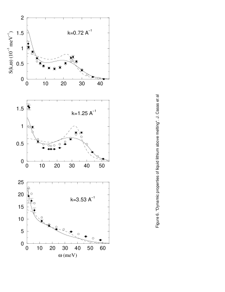
In figure 6 we show the dynamic structure factors obtained from the present formalism, along with the MD results [10], for T=470 K, and the experimental IXS data [9], measured at T=488 K, for three wave-vectors. The viscoelastic are also included for comparison. The good agreement between experiment and MD has already been remarked [9], and supports the adequacy of the potential used in order to describe the effective interaction among the ions in the liquid. It can be observed that the overall shape of is qualitatively reproduced by the present theoretical approach, in contrast with the viscoelastic model, which gives correctly the peak positions, but fails to describe the overall -dependence of the dynamic structure factor. The behavior of is of course a consequence of the time dependence of the intermediate scattering functions, . For instance, the fact that the amplitude of the decaying tail of is well reproduced implies that for small the structure factor will increase significantly, as observed in the figure. On the other hand, the deficiencies in the description of the oscillations of around the decaying tail are reflected in the less accurate representation of the Brillouin peak of .
The theoretical results for as a function of , at some fixed -values, for liquid lithium at the three temperatures, are shown in figures 7-8, where they are compared with both the corresponding MD and experimental data [1, 2, 3]. First, it is observed that the MD results show a good agreement with the experimental data, except for some discrepancies appearing at the frequency region close to . Although these discrepancies could be ascribed to the NPA interatomic pair potential used in the simulations, this may not be the ultimate reason; in fact similar problems have also been encountered by Torcini et al [26] in a similar MD study carried out with the interatomic pair potentials proposed by Price et al [40]. Moreover, it must be reminded that an accurate experimental determination of the spectral features near is not a trivial task and, therefore, the above mentioned discrepancies between MD and experiment must be taken with some caution.
On the other hand, the comparison MD/theory shows that the present theory accounts rather well for the simulation results, except in the frecuency region close to . However, this problem has to be discussed in terms of both and whose combination, according to equation (1), gives rise to the . It is observed that for , the main contribution to the comes from the , for it is the the one which dominates the whereas for both contributions to the are rather similar. Now, when the theoretical are compared with their MD counterparts, it is found that the theory can reproduce the MD results, except at the region close to where the theoretical values are always systematically lower; in fact, this is a well known deficiency of the gaussian approximation used to calculate the self-intermediate scattering function. On the other hand, the theoretical somewhat overestimates the MD values near , and therefore, this explains why the theoretical are sistematically smaller than their MD counterparts except for those -values around .
In the figures 7-8 we have also included the theoretical results obtained within the simple viscoelastic approximation. It is observed that the agreement with the MD results is very similar to that obtained with the present theory, although now the values for tend to be slightly smaller. This is again, basically, due to the corresponding which when calculated by the gaussian approximation incorporates a VACF which gives a bigger diffusion coefficient. This implies that decreases faster and leads to a smaller . Moreover, the values of are also too low, which reinforces the tendency to produce smaller
D Shear viscosity.
Figure 9 shows, for T=470 and 574 K, the MD results obtained for the SACF along with its three contributions. Note that, according to these results, the contributions from both the potential-kinetic, , and kinetic-kinetic, , parts of the SACF are negligible (less that of the potential-potential part) and therefore it justifies to restrict the theoretical calculations to the purely potential part of the SACF, as suggested in the theoretical framework presented in section II D.
In the figure, we have also plotted the theoretical along with its binary and mode-coupling components. Whereas the binary part alone is quite unable to describe the behaviour of , the inclusion of the mode-coupling component leads to a good overall agreement with the simulation data. However, it must be stressed that the present theoretical results slightly overestimate the short time ( ps) behaviour of and this is mainly due to the binary component; more explicitly, it comes from the overestimation of the values for the . Again, we note that the choice of the squared hyperbolic secant ansatz would lead to a worse description of the binary part.
On the other hand, the behaviour for , which is completely determined by the mode-coupling component, is rather well described. The values obtained for the shear viscosity coefficient, , are presented in Table III. First, we stress that the MD results compare rather well with the corresponding experimental values [41] whereas, as expected from figure 9, the theoretical values overestimate the MD ones because of their short time behaviour.
Finally, we have also plotted in figure 9, the results obtained by the viscoelastic approximation. It is observed that it overestimates the short time behaviour whereas the long-time behaviour is slightly underestimated; both effects counteract so as to produce a shear viscosity coefficient in good agreement with the MD results.
V Conclusions.
In this paper we have evaluated several dynamical properties of liquid lithium at three different thermodynamic states. The calculations have been performed both by a theoretical framework and by MD simulations, using an interatomic pair potential derived within the Neutral Pseudoatom method.
The MD results have been compared with the experimental dynamic structure factor, , obtained by IXS [9], the total dynamic structure factor, , obtained by INS [1, 2, 3], as well as with the experimental data for the self-diffusion and shear viscosity coefficients. The overall quality of the agreement is good, supporting the idea that the interatomic pair potencial derived from the NPA method can be used to describe the dynamical properties of liquid lithium at thermodynamic states near the triple point.
However, although the MD simulations can always be used to evaluate the dynamical properties of a system, once the interatomic pair potencial is given, it is also important to have a purely theoretical formalism which, besides of complementing the MD calculations, will allow the analysis of the underlying mechanisms of motion of the particles of the system. This is a relevant aspect of the present paper, where we have presented a whole theoretical framework which, by incorporating mode-coupling concepts, allows the self-consistent determination of single particle properties, as represented by the velocity autocorrelation function, its memory function, the self-diffusion coefficient and the self-dynamic structure factor, as well as collective properties such as the intermediate scattering function, the dynamic structure factor, the autocorrelation function of the non-diagonal elements of the stress tensor and the shear viscosity coefficient. The application of this theoretical framework to the study of liquid lithium at thermodynamic conditions not far from the triple point, leads to results in overall good agreement with both the corresponding MD results and the experimental data. This agreement is particularly satisfactory at the melting point whereas some deviations appear at the highest temperature investigated.
We have shown that the deficiencies in the VACF memory function, observed in previous works and related to the use of the viscoelastic model for the intermediate scattering functions, are now significantly reduced, leading to a much better description of the long time tail of . This is basically due to the improved description of the intermediate scattering functions, , in particular, of the overall amplitude of its decaying tail. However, although the present theoretical scheme accounts for these features of both the single particle and the collective dynamics, there is still room for improvement in some dynamical magnitudes, like , for which we find some discrepancies in the amplitude of the oscillations in the tail as compared with the corresponding MD results, which are also reflected in the less accurate description of the side peak of the dynamic structure factor.
Within the present theoretical framework, a key role is played by the memory functions; therefore, it is important to provide an accurate description of these magnitudes. Concerning the memory functions given in equations (6) and (28), this work shows that its short time behaviour is reasonably described by means of the gaussian ansatz. We have verified that, within the approximations made in the present work, the hyperbolic secant squared ansatz leads to results which are too wide as compared with the MD data.
As a final comment, we note that some authors [22] have used a simplified expresion for the relaxation time of the binary part of the second order memory function of the intermediate scattering functions. Instead of using the which gives the correct sixth moment of , they proposed to use the simpler , which gives the correct sixth moment of . Certainly, the values of oscillate around those of [22], but we have found that the influence of using is not negligible, giving a noticeably worse description of the intermediate scattering functions.
We end up by signaling the limitations of the formalism presented here. First, its density/temperature range of applicability lies within the region where the relevant slow relaxation channel is provided by the coupling to density fluctuations, and this ceases to be valid for densities smaller than those typical of the melting point. For these densities, coupling to other modes, like longitudinal and/or transverse currents, becomes increasingly important and we believe that this is the main reason for the small deviations observed in the VACF total memory function at the two higher temperatures studied. Moreover, we consider that an improvement in the description of the intermediate scattering function, , at all temperatures, would also require the inclusion of other modes in the corresponding second-order memory function.
Second, the theory treats in a different way the self intermediate scattering function on one hand and the velocity autocorrelation function and the intermediate scattering function on the other, since the mode-coupling effects are included for the latters but not for the first. It would clearly be desirable a more symmetric treatment, and further work is currently performed in that direction, and the results will be reported in due time.
Acknowledgements.
This work has been supported by the DGICYT of Spain (Project PB95-0720-CO2) and the Junta de Castilla y Leon (Project VA70/99). Dr. M.M.G. Alemany is kindly acknowledged for his help on the MD simulations.
REFERENCES
- [1] P. H. K. de Jong, Ph.D. Thesis (unpublished) Technische Universiteit Delft, 1993; P. Verkerk, P. H. K. de Jong, M. Arai, S. M. Bennington, W. S. Howells and A. D. Taylor, Physica B 180-181, 834 (1992)
- [2] P. H. K. de Jong, P. Verkerk, S. Ahda and L. A. de Graaf, Recent Developements in the Physics of Fluids edited by W. S. Howells and A. K. Soper (Bristol: Adam Hilger, 1992)
- [3] P. H. K. de Jong, P. Verkerk and L. A. de Graaf, J. Phys.: Condens. Matter 6, 8391 (1994); J. Non-Cryst. Solids 156, 48 (1993)
- [4] C. Morkel and W. Glaser, Phys. Rev. A 33, 3383 (1986); C. Morkel, C. Gronemeyer, W. Glaser and J. Bosse, Phys. Rev. Lett. 58, 1873 (1987)
- [5] C. Pilgrim, R. Winter, F. Hensel, C. Morkel and W. Glaser, Recent Developements in the Physics of Fluids edited by W. S. Howells and A. K. Soper (Bristol: Adam Hilger, 1992)
- [6] C. Morkel and T. Bodensteiner, J. Phys.: Condens. Matter 2, SA251 (1990); T. Bodensteiner, C. Morkel, W. Glaser and B. Dorner, Phys. Rev. A 45, 5709 (1992)
- [7] J. Seldmeier, Ph.D. Thesis (unpublished) Technische Universität München, Germany, 1992
- [8] H. Sinn and E. Burkel, J. Phys.: Condens. Matter 8, 9369 (1996)
- [9] H. Sinn, F. Sette, U. Bergmann, Ch. Halcoussis, M. Krisch, R. Verbeni and E. Burkel, Phys. Rev. Lett. 78, 1715 (1997)
- [10] M. Canales, L. E. González and J. A. Padró, Phys. Rev. E 50, 3656 (1994)
- [11] F. Shimojo, K. Hoshino and M. Watabe, J. Phys. Soc. Japan 63, 1821 (1994)
- [12] G. Kahl and S. Kambayashi, J. Phys.: Cond. Matter 6, 10897 (1994); G. Kahl, J. Phys.: Condens. Matter 6, 10923 (1994)
- [13] U. Balucani, A. Torcini and R. Vallauri, Phys. Rev. A 46, 2159 (1992)
- [14] U. Balucani, A. Torcini and R. Vallauri, J. Non-Cryst. Solids 156, 43 (1993); Phys. Rev. B 47, 3011 (1993)
- [15] M. M. G. Alemany, J. Casas, C. Rey, L. E. Gonzalez and L. J. Gallego, Phys. Rev. E 56 , 6818 (1997)
- [16] W. Gudowski, M. Dzugutov and K. E. Larsson, Phys. Rev E 47, 1693 (1993)
- [17] W. Götze and M. Lücke, Phys. Rev. A 11, 2173 (1975); M. H. Ernst and J.R. Dorfman, J. Stat. Phys. 12, 7 (1975); J. Bosse, W. Götze and M. Lücke, Phys. Rev. A 17, 434 (1978); I. M. de Schepper and M. H. Ernst, Physica A 98, 189 (1979)
- [18] A. Sjölander Amorphous and Liquid Materials edited by E. Lüscher, G. Fritsch and G. Jacucci (Dordrecht: Martinus Nijhoff, 1987)
- [19] L. Sjögren and A. Sjölander, J. Phys. C 12, 4369 (1979)
- [20] L. Sjögren, J. Phys. C 13, 705 (1980)
- [21] L. Sjögren, Phys. Rev. A 22, 2866 (1980)
- [22] L. Sjögren, Phys. Rev. A 22, 2883 (1980)
- [23] U. Balucani and M. Zoppi Dynamics of the Liquid State (Oxford, Clarendon, 1994)
- [24] U. Balucani, R. Vallauri, T. Gaskell and S. F. Duffy, J. Phys.: Condens. Matter 2, 5015 (1990)
- [25] L. E. González, D. J. González and M. Canales, Z. Phys. B 100, 601 (1996)
- [26] A. Torcini, U. Balucani, P. H. K. de Jong and P. Verkerk, Phys. Rev. E 51, 3126 (1995)
- [27] W. van der Lugt and B. P. Alblas, Handbook of Thermodynamic and Transport Properties of Alkali Metals edited by R. W. Ohse (Oxford: Blackwell, 1985)
- [28] L. E. González, D. J. González, M. Silbert and J. A. Alonso, J. Phys: Condens. Matter 5, 4283 (1993)
- [29] M. Canales, J. A. Padró, L. E. González and A. Giró, J. Phys: Condens. Matter 5, 3095 (1993)
- [30] J. R. D. Copley and S. W. Lovesey, Rep. Prog. Phys. 38, 461 (1975)
- [31] S. W. Lovesey, J. Phys. C 4, 3057 (1971)
- [32] D. Levesque and L. Verlet, Phys. Rev. A 2, 2514 (1970)
- [33] U. Balucani, Mol. Phys. 71, 123 (1990)
- [34] D. Beeman, J. Comput. Phys. 20, 130 (1976)
- [35] M. P. Allen and D. J. Tildesley, Computer Simulation of Liquids (Oxford: Clarendon, 1987)
- [36] G. A. Evangelakis, J. P. Rizos, I. E. Lagaris and I. N. Demetropoulos, Comput. Phys. Commun. 46, 401 (1987)
- [37] Y. Rosenfeld, J. Stat. Phys. 42, 437 (1986)
- [38] L. E. González, D. J. González and M. Silbert, Phys. Rev. A 45, 3803 (1992)
- [39] L. Löwenberg and A. Lodding, Z. Naturforsch. A 22, 2077 (1967)
- [40] D. L. Price, K. S. Singwi and M. P. Tosi, Phys. Rev. B 2, 2983 (1970)
- [41] E. E. Shpil’rain, K. A. Yakimovich, V. A. Fomin, S. N. Skovorodjko and A. G. Mozgovoi, Handbook of Thermodynamic and Transport Properties of Alkali Metals edited by R. W. Ohse (Oxford: Blackwell, 1985)
- [42] J. S. Murday and R. M. Cotts, Z. Naturforsch. A 26, 85 (1971)


at T=488 K


| T (K) | |||
|---|---|---|---|
| (Å-3) |
| T (K) | |||
|---|---|---|---|
| T (K) | |||
|---|---|---|---|