A thermal model for adaptive competition in a market

Abstract

Abstract: New continuous and stochastic extensions of the minority game, devised as a fundamental model for a market of competitive agents, are introduced and studied in the context of statistical physics. The new formulation reproduces the key features of the original model, without the need for some of its special assumptions and, most importantly, it demonstrates the crucial role of stochastic decision-making. Furthermore, this formulation provides the exact but novel non-linear equations for the dynamics of the system.

There is currently much interest in the statistical physics of non-equilibrium frustrated and disordered many-body systems [2]. Even relatively simple microscopic dynamical equations have been shown to lead to complex co-operative behaviour. Although several of the interesting examples are in areas traditionally viewed as physics, it is growingly apparent that many further challenges for statistical physics have their origins in other fields like biology [3] and economics [4]. In this letter we discuss a simple model whose origin lies in a market scenario and show that not only does it exhibit interesting behaviour in its own right but also it yields an intriguingly unusual type of stochastic micro-dynamics of potentially more general interest.

The model we will introduce is based on the the minority game (MG) [5], which is a simple and intuitive model for the behaviour of a group of agents subject to the economic law of supply and demand, which ensures that in a market the profitable group of buyers or sellers of a commodity is the minority one [6]. From the perspective of statistical physics, these problems are novel examples of frustrated and disordered many-body systems. Agents do not interact directly but with their collective action determine a ‘price’ which in turn affects their future behaviour, so that minority reward implies frustration. Quenched disorder enters in that different agents respond in different ways to the same stimuli. There are effective random interactions between agents via the common stimuli and the cooperative behaviour is reminiscent of that of spin-glasses [7], but there are important conceptual and technical differences compared with the problems of conventional statistical physics.

The setup of the MG in the original formulation of [5] is the following: $N$ agents choose at each time step whether to ‘buy’ ($0$) or ‘sell’ ($1$). Those agents who have made the minority choice win, the others lose. In order to decide what to do agents use strategies, which prescribe an action given the set of winning outcomes in the last $m$ time steps. At the beginning of the game each agent draws $s$ strategies randomly and keep them forever. As they play, the agents give points to all their strategies according to their potential success in the past, and at each time step they employ their currently most successful one (i.e. the one with the highest number of points).

The most interesting macroscopic observable in the MG is the fluctuation $\sigma$ of the excess of buyers to sellers. This quantity is equivalent to the price volatility in a financial context and it is a measure of the global waste of resources by the community of the agents. We therefore want $\sigma$ to be as low as possible. An important feature of the MG, observed in simulations [8], is that there is a regime of the parameters where $\sigma$ is smaller than the value $\sigma_{r}$ which corresponds to the case where each agent is buying or selling randomly. Previous studies have considered this feature from a geometrical and phenomenological point of view [9]. Our aim, however, is to enable a full analytic solution.

One of the major obstacles to an analytic study of the MG in its original formulation is the presence of an explicit time feedback via the memory $m$. Indeed, when the information processed at each time step by the agents is the true history, that is the result of the choices of the agents in the $m$ previous steps, the dynamical evolution of the system is non-Markovian and an analytic approach to the problem is very difficult.

A step forward in the simplification of the model has been made in [10], where it has been shown that the explicit memory of the agents is actually irrelevant for the global behaviour of the system: when the information processed by the agents at each time step is just invented randomly, having nothing to do with the true time series, the relevant macroscopic observables do not change. The significance of this result is the following: the crucial ingredient for the volatility to be reduced below the random value appears to be that the agents must all react to the same piece of information, irrespective of whether this information is true or false [11]. This result has an important technical consequence, since the explicit time feedback introduced by the memory disappears: the agents respond now to an instantaneous random piece of information, i.e. a noise, so that the process has become stochastic and Markovian.

The model can be usefully simplified even further and at the same time generalized and made more realistic. Let us first consider the binary nature of the original MG. It is clear that from a simulational point of view a binary setup offers advantages of computational efficiency, but unfortunately it is less ideally suited for an analytic approach [12]. More specifically, if we are interested in the analysis of time evolution, integer variables are usually harder to handle. Moreover, the geometrical considerations that have been made on a hypercube of strategies of dimension $2^{m}$ for the binary setup [9], become more natural and general if the strategy space is continuous. Finally, in the original binary formulation of the MG there is no possibility for the agents to fine tune their bids: each agent can choose to buy or sell, but they cannot choose by how much. As a consequence, also the win or loss of the agents is not related to the consistency of their bids. This is another unrealistic feature of the model, which can be improved. For all these reasons, we shall now introduce a continuous formulation of the MG.

Let us define a strategy $\vec{R}$ as a vector in the real space ${\mathbb{R}}^{D}$, subject to the constraint, $\|\vec{R}\|=\sqrt{D}.$ In this way the space of strategies $\Gamma$ is just a sphere and strategies can be thought as points on it. The next ingredient we need is the information processed by strategies. To this aim we introduce a random noise $\vec{\eta}(t)$, defined as a unit-length vector in ${\mathbb{R}}^{D}$, which is $\delta$-correlated in time and uniformly distributed on the unit sphere. Finally, we define the response $b(\vec{R})$ of a strategy $\vec{R}$ to the information $\vec{\eta}(t)$, as the projection of the strategy on the information itself,

$$b(\vec{R})\equiv\vec{R}\cdot\vec{\eta}(t)\ .$$ (1)

This response is nothing else than the bid prescribed by the particular strategy $\vec{R}$. The bid is now a continuous quantity, which can be positive (buy) or negative (sell).

At the beginning of the game each agent draws $s$ strategies randomly from $\Gamma$, with a flat distribution. All the strategies initially have zero points and in operation the points are updated in a manner discussed below. At each time step the agent uses his/her strategy with the highest number of points. The total bid is:

$$A(t)\equiv\sum_{i=1}^{N}b_{i}(t)=\sum_{i=1}^{N}\vec{R}^{\star}_{i}(t)\cdot\vec{\eta}(t)\ ,$$ (2)

where $\vec{R}^{\star}_{i}(t)$ is the best strategy (that with the highest number of points) of agent $i$ at time $t$.

We have now to update the points. This is particularly simple in the present continuous formulation. Let us introduce a time dependent function $P(\vec{R},t)$ defined on $\Gamma$, which represents the points $P$ of strategy $\vec{R}$ at time $t$. We can write a very simple and intuitive time evolution equation for $P$,

$$P(\vec{R},t+1)=P(\vec{R},t)-A(t)\,b(\vec{R})/N\ ,$$ (3)

where $A(t)$ is given by eq.(2). A strategy $\vec{R}$ is thus rewarded (penalized) if its bid has an opposite (equal) sign to the total bid $A(t)$, as the supply-demand dynamics requires. Now the win or the loss is proportional to the bid.

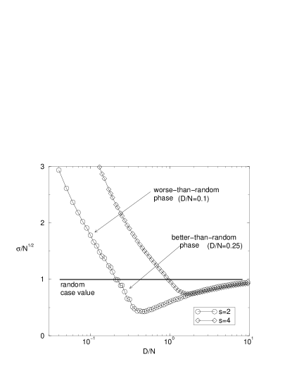
FIG. 1.: Continuous formulation: The scaled variance $\sigma/\sqrt{N}$ as a function of the reduced dimension $D/N$, at $s=2$ and $s=4$. The horizontal line is the variance in the random case. The total time $t$ and the initial time $t_{0}$ are $10000$ steps. Average over $100$ samples, $N=100$.

It is important to check whether the results obtained with this continuous formulation of the MG are the same as in the original binary model. The main observable of interest is the variance (or volatility) $\sigma$ in the fluctuation of $A$, $\sigma^{2}=\lim_{t\to\infty}\frac{1}{t}\int_{t_{0}}^{t_{0}+t}dt^{\prime}\;A(t^{\prime})^{2}$. Indeed, we shall not consider any quantity related to individual agents. We prefer to concentrate on the global behaviour of the system, taking more the role of the market regulator than that of a trading agent. The main features of the MG are reproduced: first, we have checked that the relevant scaling parameter is the reduced dimension of the strategy space $d=D/N$; second, there is a regime of $d$ where the variance $\sigma$ is smaller than the random value $\sigma_{r}$, showing a minimum at $d=d_{c}(s)$, and, moreover, the minimum of $\sigma(d)$ is shallower the higher is $s$ [9]; see Fig.1. It can be shown that all the other standard features of the binary model are reproduced in the continuous formulation.

An interesting observation is that there is no need for $\vec{\eta}(t)$ to be random at all. Indeed, the only requirement is that it must be ergodic, spanning the whole space $\Gamma$, even in a deterministic way. Moreover, if $\vec{\eta}(t)$ visits just a sub-space of $\Gamma$ of dimension $D^{\prime}<D$ everything in the system proceeds as if the actual dimension was $D^{\prime}$: the effective dimension of the strategy space is fixed by the dimension of the space spanned by the information.

Relations (2) and (3) constitute a closed set of equations for the dynamical evolution of $P(\vec{R},t)$, whose solution, once averaged over $\vec{\eta}$ and over the initial distribution of the strategies, gives in principle an exact determination of the behaviour of the system. In practice, the presence of the ‘best-strategy’ rule, i.e. the fact that each agent uses the strategy with the highest points, makes the handling of these equations still difficult. From the perspective of statistical physics it is natural to modify the deterministic nature of the above procedure by introducing a thermal description which progressively allows stochastic deviations from the ‘best-strategy’ rule, as a temperature is raised. We shall see that this generalization is also advantageous, both for the performance of the system in certain regimes and for the development of convenient analytical equations for the dynamics. In this context the ‘best-strategy’ original formulation of the MG can be viewed as a zero temperature limit of a more general model.

Hence we introduce the Thermal Minority Game (TMG), defined in the following way. We allow each agent a certain degree of stochasticity in the choice of the strategy to use at any time step. For each agent $i$ the probabilities of employing his/her strategy $a=1,\dots,s$ is given by,

$$\pi^{a}_{i}(t)\equiv\frac{e^{\beta P(\vec{R}_{i}^{a},t)}}{Z_{i}}\ ,\ \ \ \ Z_{i}\equiv\sum_{b=1}^{s}e^{\beta P(\vec{R}_{i}^{b},t)}\ ,$$ (4)

where $P$ are the points, evolving with eq.(3). The inverse temperature $\beta=1/T$ is a measure of the power of resolution of the agents: when $\beta\to\infty$ they are perfectly able to distinguish which is their best strategy, while for decreasing $\beta$ they are more and more confused, until for $\beta=0$ they choose their strategy completely at random. What we have defined is therefore a model which interpolates between the original ‘best-strategy’ MG ($T=0$, $\beta=\infty$) and the random case ($T=\infty$, $\beta=0$). In the language of Game Theory, when $T=0$ agents play ‘pure’ strategies, while at $T>0$ they play ‘mixed’ ones [13].

We now consider the consequences of having introduced the temperature. Let us fix a value of $d$ belonging to the worse-than-random phase of the MG (see Fig.1) and see what happens to the variance $\sigma$ when we switch on the temperature. We do know that for $T=0$ we must recover the same value as in the ordinary MG, while for $T\to\infty$ we must obtain the value $\sigma_{r}$ of the random case. But in the middle a very interesting thing occurs: $\sigma(T)$ is not a monotonically decreasing function of $T$, but there is a large intermediate temperature regime where $\sigma$ is smaller than the random value $\sigma_{r}$. This behaviour is shown in Fig.2.

The meaning of this result is the following: even if the system is in a MG phase which is worse than random, there is a way to significantly decrease the volatility $\sigma$ below the random value $\sigma_{r}$ by not always using the best strategy, but rather allowing a certain degree of individual error.

FIG. 2.: TMG: The scaled variance $\sigma/\sqrt{N}$ as a function of the temperature $T$, at $D/N=0.1$, for $s=2$. In the inset we show $\sigma(T)/\sqrt{N}$ for $D/N=0.25$.

Note from Fig.2 that the temperature range where the variance is smaller than the random one is more than two orders of magnitude large, meaning that almost every kind of individual stochasticity of the agents improves the global behaviour of the system. Furthermore, as we show in the inset of Fig.2, if we fix $d$ at a value belonging to the better-than-random phase, but with $d<d_{c}$, a similar range of temperature still improves the behaviour of the system, decreasing the volatility even below the MG value.

FIG. 3.: TMG: The scaled variance $\sigma/\sqrt{N}$ as a function of the reduced dimension $D/N$, at different values of the temperature $T=2^{k}\times 10^{-2}$, for $s=2$.

These features can be seen also in Fig.3, where we plot $\sigma$ as a function of $d$ at various values of the temperature. In addition this figure shows further effects: (i) the improvement due to thermal noise occurs only for $d<d_{c}$; (ii) there is a cross-over temperature $T_{1}\sim 1$, below which temperature has very little effect for $d>d_{c}$; (iii) above $T_{1}$ the optimal $d_{c}(T)$ moves continuously towards zero and $\sigma(d_{c})$ increases; (iv) there is a higher critical temperature $T_{2}\sim 10^{2}$ at which $d_{c}$ vanishes, and for $T>T_{2}$ the volatility becomes monotonically increasing with $d$.

We turn now to a more formal description of the TMG. Once we have introduced the probabilities $\pi_{i}^{a}$ in eq.(4) we can write a dynamical equation for them. Indeed, from eq.(3), after taking the continuous-time limit, we have,

$$\dot{\pi}_{i}^{a}(t)=-\beta\;\pi_{i}^{a}(t)\;a(t)\left(\vec{R}_{i}^{a}-\sum_{b=1}^{s}\pi_{i}^{b}(t)\;\vec{R}_{i}^{b}\right)\cdot\vec{\eta}(t)\ ,$$ (5)

where the normalized total bid $a(t)$ is given by,

$$a(t)=N^{-1}\,\sum_{i=1}^{N}\vec{r}_{i}(t)\cdot\vec{\eta}(t)\ .$$ (6)

Now $\vec{r}_{i}(t)$ is a stochastic variable, drawn at each time $t$ with the time dependent probabilities set $[\pi_{i}^{1},\dots,\pi_{i}^{s}]$. Note the different notation: $\vec{R}_{i}^{a}$ are the quenched strategies, while $\vec{r}_{i}(t)$ is the particular strategy drawn at time $t$ from the set $[\vec{R}^{1}_{i},\dots,\vec{R}^{s}_{i}]$ by agent $i$ with instantaneous probabilities $[\pi^{1}_{i}(t),\dots,\pi^{s}_{i}(t)]$. In order to better understand equation (5), we recall that $b_{i}^{a}(t)=\vec{R}_{i}^{a}\cdot\vec{\eta}(t)$ is the bid of strategy $\vec{R}_{i}^{a}$ at time $t$ (eq.(1)) and therefore the quantity $w_{i}^{a}(t)\equiv-B(t)b_{i}^{a}(t)$ can be considered as the win of this strategy (cf. eq.(3)). Hence, we can rewrite eq. (5) in the following more intuitive form,

$$\dot{\pi}_{i}^{a}(t)=\beta\;\pi_{i}^{a}(t)\;[\;w^{a}_{i}(t)-\langle w\rangle_{i}\;]\ ,$$ (7)

where $\langle w\rangle_{i}\equiv\sum_{b=1}^{s}\pi_{i}^{b}(t)\;w^{b}_{i}(t)$. The meaning of equation (7) is clear: the probability $\pi^{a}_{i}$ of a particular strategy $\vec{R}^{a}_{i}$ increases only if the performance of that strategy is better than the instantaneous average performance of all the strategies belonging to the same agent $i$ with the same actual total bid [14].

Relations (5) and (6) are the exact dynamical equations for the TMG. They do not involve points nor memory, but just stochastic noise and quenched disorder, and they are local in time. From the perspective of statistical mechanics, this is satisfying and encouraging. However, these equations differ fundamentally from conventional replicator and Langevin dynamics. First, the Markov-propagating variables are themselves probabilities. Second, there are two sorts of stochastic noises, as well as quenched randomness. Third, and more importantly, the stochastic noises enter non-linearly, one independently for each agent via probabilistic dependence on the $\pi$ themselves, the other globally and quadratically. They thus provide interesting challenges for fundamental transfer from microscopic to macroscopic dynamics, including an identification of the complete set of necessary order parameters [15]. We shall address the problem of finding a solution of the TMG equations in a future work.

Finally, let us note that the TMG (as well as the MG) is not only suitable for the description of market dynamics. Indeed, any natural system where a population of individuals must organize itself in order to optimize the utilization of some limited resources, is qualitatively well described by such a model. We hope that the thermal model we have introduced in this Letter will give more insight into this kind of natural phenomena.

We thank L. Billi, P. Gillin and P. Love for many suggestions, and N.F. Johnson and I. Kogan for useful discussions. This work was supported by EPSRC Grant GR/M04426 and EC Grant ARG/B7-3011/94/27.

REFERENCES

- [1]
- [2] See, for example, J.-P. Bouchaud, L.F. Cugliandolo, J. Kurchan and M. Mézard in Spin Glasses and Random Fields, edited by A.P. Young, (World-Scientific, Singapore, 1998); Nonequilibrium Statistical Mechanics in One Dimension, edited by V. Privman, (Cambridge University Press, 1997).
- [3] See, for example, Physics of Biomaterials, edited by T. Riste and D. Sherrington, (Kluwer Academic Press, Dordrecht, 1996); Landscape Paradigms in Physics and Biology, edited by H. Frauenfelder et al., (North-Holland, Amsterdam, 1997).
- [4] The Economy as an Evolving Complex System, edited by P.W. Anderson, K. Arrow and D. Pines (Addison-Wesley, Redwood City, 1988).
- [5] D. Challet and Y.-C. Zhang, Physica A 246, 407 (1997).
- [6] See e.g. W.B. Arthur, Amer. Econ. Assoc. Papers and Proc. 84, 406 (1994); Science, 284, 107 (1999).
- [7] M. Mézard, G. Parisi and M. A. Virasoro, Spin Glass Theory And Beyond (World Scientific, Singapore, 1986).
- [8] R. Savit, R. Manuca and R. Riolo, Phys. Rev. Lett. 82, 2203 (1999).
- [9] D. Challet and Y.-C. Zhang, Physica A 256, 514 (1998); Y.-C. Zhang, Europhys. News 29, 51 (1998); N.F. Johnson, M. Hart and P.M. Hui, Physica A, 269, 1 (1999); R. D’hulst and G.J. Rodgers, Physica A, 270, 222 (1999).
- [10] A. Cavagna, Phys. Rev. E, 59, R3783 (1999).
- [11] In economics such a situation is described as sun-spot equilibrium; see e.g. M. Woodford, Econometrica, 58, 277 (1990). (We thank M. Marsili for drawing our attention to sun-spots.)
- [12] See, however, D. Challet and M. Marsili, cond-mat/9904071.
- [13] J. Hofbauer and K. Sigmund, Evolutionary Games and Population Dynamics, (Cambridge University Press, 1998).
- [14] Equations (7) are not replicator equations [13]. The latter describe deterministic processes, while eqs.(7) correspond to a dynamics which involves two sorts of stochastic noise, together with quenched disorder. Stochastic learning processes are described by replicator equations only if the continuous-time limit is taken in a particular way; see T. Börgers and R. Sarin, J. Econ. Theory, 77, 1 (1997).
- [15] A.C.C. Coolen, S.N. Laughton and D. Sherrington, Phys. Rev. B 53, 8184 (1996).