On the properties of small-world network models

Abstract

We study the small-world networks recently introduced by Watts and Strogatz [Nature 393, 440 (1998)], using analytical as well as numerical tools. We characterize the geometrical properties resulting from the coexistence of a local structure and random long-range connections, and we examine their evolution with size and disorder strength. We show that any finite value of the disorder is able to trigger a “small-world” behaviour as soon as the initial lattice is big enough, and study the crossover between a regular lattice and a “small-world” one. These results are corroborated by the investigation of an Ising model defined on the network, showing for every finite disorder fraction a crossover from a high-temperature region dominated by the underlying one-dimensional structure to a mean-field like low-temperature region. In particular there exists a finite-temperature ferromagnetic phase transition as soon as the disorder strength is finite.

PACS numbers: 05.50.+q 64.60.C 05.70.Fh

I Introduction

A recent article by Watts and Strogatz [2], showing the relevance of what they called “small-world” networks for many realistic situations, has triggered a lot of attention for these kind of networks [3, 4, 5, 6, 7, 8]: this interest results from their very definition, allowing an exploration between regular and random networks.

Random networks have of course been the subject of many studies in various domains, ranging from physics to social sciences. A very important characteristic common to such lattices and for example social networks is that the length of the shortest chain connecting two vertices (or members) grows very slowly, i.e. in general logarithmically, with the size of the network [9]. This characteristic has important consequences for many issues, e.g. the speed of disease spreading [2] etc. The social psychologist S. Milgram [10], after realizing that the number of persons necessary to link two randomly chosen, geographically separated persons had a median number of six, has called this concept the “six degrees of separation”. In addition, models defined on random networks are, due to their locally tree-like structure, of mean-field type, and can therefore be analytically more tractable than their counterparts defined on regular lattices, but, thanks to the finite connectivity of their vertices, they display however behaviours which are intrinsically not captured by the familiar infinite connectivity models [11].

However, it is well known that many realistic networks have a local structure which is very different from random networks with finite connectivity. For example, two neighbours have many common neighbours, a property which does not hold for random networks, and which can be quantified by the introduction of the “clustering coefficient” (see section III). Such phenomena are not only found in social networks, but also e.g. in the connections of neural networks [2] or in the chemical bond structure of long macromolecules [12]: The one-dimensional couplings of neighbouring monomers are complemented by long-ranged interactions between monomers that are close in space although not along the chain. This interplay has been studied in fact for example in [13], but it seems that, in this case, the long-range interactions are not sufficient to really modify the properties of the one-dimensional structure of the chain .

The construction proposed by Watts and Strogatz [2], that we will recall in section II, allows to reconcile local properties of a regular network with global properties of a random one, by introducing a certain amount of random long-range connections into an initially regular network.

The aim of this paper is to study in some detail the concepts used in [2] to characterize the “small-world” behaviour, caused by the coexistence of “short-range” and “long-range” connections. We will show that this behaviour does not appear at a finite value of the disorder $p$, but that, for any $p>0$, the networks will display this behaviour as soon as their size is large enough.

This paper is organized as follows. In section II we describe the procedure used to obtain small-world networks; in section III we study some of their geometrical properties, i.e. the connectivity, the chemical distances and the “clustering” coefficient, analytically as well as numerically . Section IV contains the investigation of an Ising-model defined on a small-world lattice, where the interplay between the short- and long-range interactions leads to interesting physical effects.

II Definition of the model(s)

The construction algorithm proposed by Watts and Strogatz for small-world networks is the following: the initial network is a one-dimensional lattice of $N$ sites, with periodic boundary conditions (i.e. a ring), each vertex being connected to its $2k$ nearest neighbours. The vertices are then visited one after the other; each link connecting a vertex to one of its $k$ nearest neighbours in the clockwise sense is left in place with probability $1-p$, and with probability $p$ is reconnected to a randomly chosen other vertex. Long range connections are therefore introduced. Note that, even for $p=1$, the network keeps some memory of the procedure and is not locally equivalent to a random network: each vertex has indeed at least $k$ neighbours. An important consequence is that we have no isolated vertices, and the graph has usually only one component (a random graph has usually many components of various sizes).

FIG. 1.: Examples of networks obtained by the procedure described in the text, for $k=2$, $N=20$. (a): $p=0$, regular networks; (b), (c): intermediate values of $p$; (d): $p=1$.

It is possible to obtain “small-world” networks in other ways, that yields the same physical consequences, and can be more tractable analytically. For example, the networks studied in [5, 6] are obtained by adding long-range connections to the initial ring without diluting its one-dimensional structure; the mean connectivity then changes with the disorder. In section IV we will also study an initial network with multiple links between successive vertices.

III Geometrical properties

A Connectivity

For $p=0$, each vertex has the same connectivity $2k$. On the other hand, a non-zero value of $p$ introduces disorder into the network, in the form of a non-uniform connectivity, while maintaining a fixed average connectivity $\bar{c}=2k$. Let us denote $P_{p}(c)$ the probability distribution of the connectivities.

Since $k$ of the initial $2k$ connections of each vertex are left untouched by the construction, the connectivity of a vertex $i$ can be written $c_{i}=k+n_{i}$, with $n_{i}\geq 0$. $n_{i}$ can then again be divided in two parts: $n_{i}^{1}\leq k$ links have been left in place (each one with probability $1-p$), the other $n_{i}^{2}=n_{i}-n_{i}^{1}$ links have been reconnected towards $i$, each one with probability $p/N$. We readily obtain

$$P_{1}(n_{i}^{1})={k\choose n_{i}^{1}}(1-p)^{n_{i}^{1}}p^{k-n_{i}^{1}}$$ (1)

$$P_{2}(n_{i}^{2})=\frac{(kp)^{n_{i}^{2}}}{n_{i}^{2}!}\exp{(-pk)}\ \ \ \ \ \ \mbox{ for large $N$}$$ (2)

and find

$$P_{p}(c)=\sum_{n=0}^{\min(c-k,k)}{k\choose n}(1-p)^{n}p^{k-n}\frac{(kp)^{c-k-n}}{(c-k-n)!}\exp{(-pk)},\ \ \ c\geq k.$$ (3)

We show in figure (2) the probability distributions for $k=3$ and various values of $p$: as $p$ grows, the distribution becomes broader.

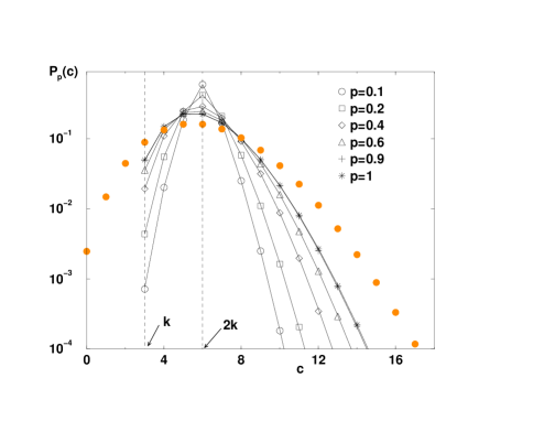
FIG. 2.: Probability distributions of the connectivity $c$ for $k=3$ and various values of $p$: $c\geq k$, and the mean connectivity is $\bar{c}=2k=6$. The symbols are obtained by numerical simulations of small-world networks (with $N=1000$ vertices), and the lines are a guide to the eye, joining points given by formula (3). Filled circles show the probability distribution of the connectivity $c$ for a random network of mean connectivity is $\bar{c}=2k=6$ (given by $(2k)^{c}\exp(-2k)/c!$).

B Chemical distances

We now turn to a non-local quantity of graphs: the chemical distance between its vertices, i.e. the minimal number of links between two vertices. We note $d_{ij}$ the chemical distance between vertices $i$ and $j$, and

$$\ell(N,p)=\frac{1}{N(N-1)}\overline{\sum_{i\neq j}d_{ij}}$$ (4)

the mean chemical distance, averaged over all pairs of vertices and over the disorder induced by the rewiring procedure.

Watts and Strogatz have shown that the mean distance between vertices $\ell(N,p)$ decreases very rapidly as soon as $p$ is non-zero. They however show the curve of $\ell(N,p)$ versus $p$ for only one value of $N$ and do not study how it depends on $N$. For $p=0$, we have a linear chain of sites, so that we easily find

$$\ell(N,0)=\frac{N(N+2k-2)}{4k(N-1)}\sim\frac{N}{4k},$$ (5)

growing like $N$. On the other hand, for $p=1$ $\ell(N,1)$ grows like $\ln(N)/\ln(2k-1)$ (inset of figure (3)): the graph is then random. Besides, the distribution of lengths, being uniform between $1$ (shortest possible distance) and $N/(2k)$ for the linear chain, becomes more and more peaked around its mean value as $p$ grows (see figure (3)).

It is therefore quite natural to ask if the change between these two behaviours occurs by a transition at a certain finite critical value of $p$ or if there is a crossover phenomenon at any finite value of $N$, with a transition occurring only at $p=0$. This last scenario was first proposed in [3].

FIG. 3.: Probability distribution of the distance $d_{ij}$ between two vertices $i$ and $j$ of small-world graphs, for $k=3$, $N=2000$, $p=2^{-20}$ (flat distribution), $p=2^{-12},\ 2^{-10}$ and $2^{-8}$ (curves becoming more and more peaked as $p$ grows), averaged over $500$ samples for each $p$. The maximum value of $d_{ij}$ is of course $N/(2k)$. Inset: $\ell(N,1)$ versus $N$ for $k=3$ and $k=5$, together with the $\ln(N)/\ln(2k-1)$ straight lines.

We first investigate this question by numerical simulations, to study the behaviour of $\ell(N,p)$ in a systematic way, varying $N$ and $p$: we use values of $N$ from $100$ to $20000$, with $p=2^{a}/2^{20}$, $a=0,\cdots,20$, and we average over $500$ realizations of the disorder for each value of $p$. We have studied three different values of the mean connectivity: $2k=4,\ 6$ and $10$.

In figure (4), we plot $\ell(N,p)/\ell(N,0)$ for various values of $N$ and $k=2$. It is clear that $\ell(N,p)$ decreases very fast already for small $p$ (note the logarithmic scale for $p$): from this point of view, the network is very soon similar to a random network. In particular, as $N$ becomes larger, the drop in the curve occurs for smaller and smaller values of $p$, showing that no finite critical value of $p$ can be determined this way: in the thermodynamic limit, $\ell(N,p)/\ell(N,0)$ goes to $0$ for all $p>0$. This is a first clear indication of a crossover behaviour (as opposed to a transition at a non-zero $p$) that we are now going to examine in more details.

Note that the first evidence of a crossover has been given in [3] by the numerical study of system with sizes up to $N=1000$, and mean connectivities $2k=10,\ 20,\ 30$. A scaling of the form

$$\ell(N,p)\sim N^{*}F_{k}\left(\frac{N}{N^{*}}\right)$$ (6)

was proposed, where $F_{k}$ depends only on $k$, with $F_{k}(u\ll 1)\sim u$, $F_{k}(u\gg 1)\sim\ln u$, and $N^{*}\sim p^{-\tau}$ with $\tau=2/3$ as $p$ goes to zero. However, it can be shown [4], with a simple but rigorous argument, that $\tau$ cannot in fact be lower than $1$: the mean number of rewired links is $N_{r}=pNk$; if $\tau<1$, and if we take $\alpha$ such that $\tau<\alpha<1$, then the scaling hypothesis implies, for large $N$, $\ell(N,N^{-1/\alpha})\sim N^{\tau/\alpha}\ln(N)$ (since $N^{1-\tau/\alpha}\gg 1$ for large $N$); $N_{r}$ however goes to zero for large $N$, so that the rewiring of a vanishing number of links could lead to a change in the scaling of $\ell$. This obviously unphysical result shows that the hypothesis $\tau<1$ is not valid. In addition, Newman and Watts [6], using a renormalization group analysis, have shown that $\tau=1$ exactly. Here we will arrive at the same result, using our numerical simulations to test the scaling hypothesis, as well as analytical arguments.

FIG. 4.: Mean chemical length $\ell(N,p)$ normalized by $\ell(N,0)$, versus $p$, for $k=2$, and $N$ from $100$ to $20000$: the drop in the curve occurs at lower and lower values of $p$ as $N$ grows.

To understand how strong the disorder has to be to induce a crossover, and to show that this crossover can occur, at fixed $p$, for $N^{*}\sim p^{-\tau}$, or equivalently, at fixed $N$, for $p^{*}\sim N^{-1/\tau}$, only with $\tau\geq 1$, we study the case of a finite number of rewired links, $N_{r}=\alpha$. This corresponds to $p=\alpha/N$. In order to show that such a value of $p$ is not able to alter the scaling of $\ell$ with $N$, we now establish a rigorous lower bound.

For any given sample, the extremities of the $\alpha$ rewired links determine $2\alpha$ intervals. The sum of their lengths on the ring is $N$, so that at least one of them has a length of order $N$, which is, even more precisely, larger than $N/(2\alpha)$. We call this interval $J=[i_{0},j_{0}]$ and we consider the interval $I\subset J$, of length $N/(4\alpha)=bN$, $I=[i_{0}+N/(8\alpha),i_{0}+3N/(8\alpha)]$, which has not been modified by the rewiring procedure. We now decompose the mean length between two vertices of the sample,

$$\ell=\frac{1}{N(N-1)}\sum_{i\neq j}d_{ij},$$

into two contributions: the first one comes from the pairs $(i,j)$ with $i\in I,\ j\in I$, the second one includes all pairs $(i,j)$ where at least one of the vertices is not an element of $I$. The first contribution can be estimated by formula (5), since it comes from a part of the graph which has not been modified, and at a distance big enough from any modified link:

$$\sum_{i\in I,\ j\in I}d_{ij}\geq(bN)(bN-1)\frac{bN}{4k}$$

(the inequality comes from the fact that we do not have periodic boundary conditions for this interval). We now have access to a lower bound of $\ell(N,\alpha/N)$ (which is valid for any sample, and consequently also for the average over samples):

$$\ell(N,\alpha/N)\geq\frac{1}{N(N-1)}\sum_{i\in I,\ j\in I}d_{ij}\geq\frac{b^{3}}{4k}N.$$

Since $\ell(N,\alpha/N)$ is smaller than $\ell(N,0)\sim N/(4k)$, this shows that

$$\ell(N,\alpha/N)=O(N).$$ (7)

In other words, a finite number of rewired links cannot change the scaling at large $N$: $\ell(N,\alpha/N)$ is of order $N$ for any finite $\alpha$.

To complete this argument, we have computed numerically $p_{1/2}(N)$, i.e. the value of $p$ such that $\ell(N,p_{1/2}(N))=\ell(N,0)/2$. Figure (5) shows quite clearly that, for large $N$, $p_{1/2}(N)\sim 1/N$: a finite number of rewired links is able to divide the mean length between vertices by two .

FIG. 5.: $p_{1/2}(N)$ such that $\ell(N,p_{1/2}(N))=\ell(N,0)/2$, versus N, for $k=2,\ 3,\ 5$. The straight line is proportional to $1/N$.

Let us now go back to the scaling hypothesis of [3]. If the scaling form of equation (6) is valid, we have to compute $\ell(N,p)$ at fixed $p$ in order to estimate $N^{*}(p)$. For large $N$, it behaves like $N^{*}(p)\ln(N)$ (see figure (6) for different values of $p$). For small $p$, $N^{*}(p)$ becomes bigger and bigger, so that we have to use larger and larger values of $N$. We show in figure (7) that the $N^{*}(p)$ estimated in this way behaves like $1/p$ for small $p$ (and for $p\to 1$, $N^{*}(p)\to\ln(2k-1)$, in accordance with $\ell(N,1)\sim\ln(N)/\ln(2k-1)$), giving $\tau=1$. This is not very surprising if we consider the above discussion showing that a finite number of rewired links will change the coefficient of the scaling of $\ell$ with $N$ but not the scaling itself. Moreover, $p_{1/2}(N)$ corresponds to the drop in the curves of figure (4) and can therefore be considered as a crossover value.

FIG. 6.: $\ell(N,p)$ versus $N$, for $p=2^{-a}$, $a=6,\cdots,11$, and $k=3$. For large values of $p$ we have a straight line in the semi-log plot, while for small values of $p$ we observe the crossover between $\ell(N,p)\sim N$ and $\ell(N,p)\sim\ln(N)$. The value of $N^{*}(p)$ is given by the slope of the linear part in the semi-log plot.

FIG. 7.: $N^{*}(p)$ versus $p$ for $k=2,\ 3,\ 5$. The straight line is proportional to $1/p$.

Using the determined values of $N^{*}$, we plot in figure (8) $\ell(N,p)/N^{*}(p)$ versus $N/N^{*}(p)$ for various values of $N$ and $p$. We observe a nice collapse of the data for each value of $k$. Thanks to the range of values of $N$ that we use, we are able to show the collapse over a much wider range of values than [3]. We clearly see the linear behaviour $F_{k}(x\ll 1)\sim x/(4k)$, and the crossover to $F_{k}(x\gg 1)\sim\ln(x)$. Note that, as explained in [6], we have to use values of $p$ lower than $1/k^{2}$ (and of course large enough values of $N$, i.e. $N\gg k$) to obtain a clean scaling behaviour: for too large $p$, we are moving out of the scaling regime close to the $p=0$-transition.

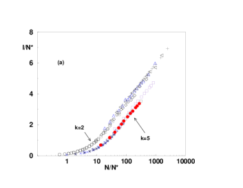
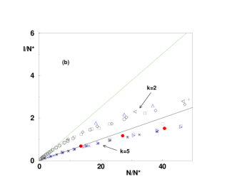
FIG. 8.: Data collapse $\ell(N,p)/N^{*}(p)$ versus $N/N^{*}(p)$, for $k=2$ and $k=5$; (a): log-linear scale showing at large $N/N^{*}$ the logarithmic behaviour; (b) linear scale showing at small $N/N^{*}$ the linear behaviour $\ell(N,p)\sim N/(4k)$: the straight lines have slopes $1/8$ and $1/20$.

C Clustering coefficient

To define the “small-world” behaviour, two ingredients are used by Watts and Strogatz [2]. The first one is the chemical length studied in the previous paragraph, which depends strongly on $p$ and $N$. The second one is more local: the “clustering coefficient” ${\cal C}(p)$ quantifies its “cliquishness”. ${\cal C}(p)$ is indeed defined as follows: if $c_{i}$ is the number of neighbours of a vertex $i$, there are a priori $c_{i}(c_{i}-1)/2$ possible links between these neighbours. Denoting ${\cal C}_{i}$ the fraction of these links that are really present in the graph, ${\cal C}(p)$ is the average of ${\cal C}_{i}$ over all vertices. On a linear-log plot, ${\cal C}(p)/{\cal C}(0)$ is close to $1$ for a wide range of values of $p$, and its drop occurs around $p\approx 0.1$. This is therefore in contrast with $\ell(N,p)$, whose drop occurs for much smaller values of $p$ as soon as $N$ is large enough. It is therefore an interesting question whether there is an upper threshold on $p$ for the small-world behaviour.

We now show that a simple redefinition of ${\cal C}(p)$ leads to a very simple formula, without altering its physical signification, nor the shape of the curve. For $p=0$, each vertex has $2k$ neighbours; it is easy to see that the number of links between these neighbours is ${\cal N}_{0}=3k(k-1)/2$. Then ${\cal C}(0)=\frac{3(k-1)}{2(2k-1)}$. For $p>0$, two neighbours of $i$ that were connected at $p=0$ are still neighbours of $i$ and linked together with probability $(1-p)^{3}$, up to terms of order $\frac{1}{N}$. The mean number of links between the neighbours of a vertex is then clearly ${\cal N}_{0}(1-p)^{3}+O(\frac{1}{N})$. The clustering coefficient ${\cal C}(p)$ is defined as the mean of the ratio ${\cal C}_{i}=\frac{{\cal N}_{i}}{c_{i}(c_{i}-1)/2}$. If instead we define $\tilde{{\cal C}}(p)$ as the ratio of the mean number of links between the neighbours of a vertex and the mean number of possible links between the neighbours of a vertex, we obtain

$$\tilde{{\cal C}}(p)=\frac{3(k-1)}{2(2k-1)}(1-p)^{3}$$ (8)

We check numerically, with $N=50$ to $N=8000$, and averaging over $5000$ samples, that the two definitions lead to the same behaviour (we see in figure (9) that the difference between ${\cal C}(p)$ and $\tilde{{\cal C}}(p)$ is very small), and that the corrections to eq. (8) are indeed of order $1/N$. The behaviour of ${\cal C}(p)$ is therefore very simply described by ${\cal C}(p)\approx{\cal C}(0)(1-p)^{3}$, and the dependence on $N$ is very small.

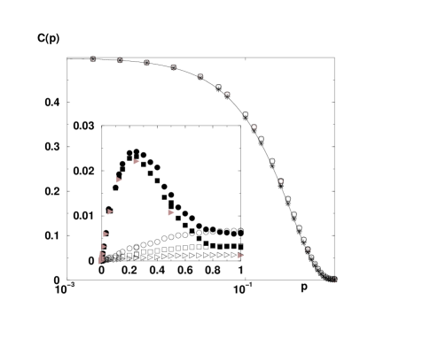
FIG. 9.: ${\cal C}(p)$ and $\tilde{{\cal C}}(p)$ versus $p$, for $k=2$ (${\cal C}(0)=\tilde{{\cal C}}(0)=0.5$), $N=1000,\ 2000,\ 5000$: open symbols are for ${\cal C}(p)$, and the crosses are for $\tilde{{\cal C}}(p)$; the line is ${\cal C}(0)(1-p)^{3}$. Inset: corrections ${\cal C}(p)-{\cal C}(0)(1-p)^{3}$ (filled symbols) for $N=1000$ (circles), $N=2000$ (squares) and $N=5000$ (triangles), and $\tilde{{\cal C}}(p)-{\cal C}(0)(1-p)^{3}$ (open symbols) for $N=1000$ (circles), $N=2000$ (squares) and $N=5000$ (triangles). We see that the corrections go to zero as $1/N$ for $\tilde{{\cal C}}(p)$; the corrections for ${\cal C}(p)$ are larger, but anyway very small.

To summarize this section, we have shown that the small-world behaviour – as defined by the average chemical distance and the clustering coefficient – is indeed present for any finite value of $0<p<1$ as soon as the network is large enough.

IV Ising model

In this section we want to investigate the consequences of the mixed geometrical structure of small-world networks on an Ising model as a prototype of statistical-mechanics models that can be defined on it. This model can be understood as a continuous interpolation of a pure one-dimensional model for $p=0$ showing no phase transition at finite temperature to a model on a random graph for $p=1$ having a finite critical temperature $T_{c}(p=1)>0$ as long as $k\geq 2$, cf. [14]. In agreement with the results from section III, we find for every finite $p>0$ that the low temperature behaviour of the model is of mean-field character, even if we observe a finite temperature crossover to a dominance of the one-dimensional structure. This observation confirms the value $p_{c}=0$ for the onset of a non-trivial thermodynamical small-world behaviour as already found in the geometrical properties, and it shows again the crucial importance of the mixed geometrical structure, as even global quantities can be dominated by the initial ordered structure for high temperatures.

A General formalism

The system we want to study is given by its Hamiltonian

$$H(\{S_{i}\})=-\sum_{i=1}^{N}S_{i}\sum_{j=1}^{k}S_{m(i,j)}$$ (9)

with $N$ Ising spins $S_{i}=\pm 1,\ i=1,...,N,$ and periodic boundary conditions, i.e. we identify $S_{N+1}=S_{1}$ etc. in the following. The independently and identically distributed numbers $m(i,j)$ are drawn from the probability distribution

$$P(m(i,j))=(1-p)\delta_{m(i,j),i+j}+\frac{p}{N}\sum_{l=1}^{N}\delta_{m(i,j),l},\$$ (10)

i.e. for $p=0$ we obtain a pure one-dimensional Ising model where every site is connected to its $2k$ nearest neighbours by ferromagnetic bonds of strength 1, whereas this structure is completely replaced by random long-range bonds for $p=1$. The number of bonds in the model is given by $kN$, independently of the disorder strength $p$. Here we consider only the case of finite probabilities $p=O(1)$, i.e. an extensive number of links is rewired and, according to the last section, we are therefore in the small-world regime.

In order to decide whether there exists a ferromagnetic phase transition at finite temperature or not, we have to calculate the free-energy density at inverse temperature $\beta$. Due to the existence of an extensive number as well of random as of one-dimensional links and due to the translational invariance of the distribution (10) we expect this quantity to be self-averaging, we therefore have to determine

$$f = -\lim_{N\to\infty}\frac{1}{\beta N}\overline{\ln Z}$$ (11)

$$= -\lim_{N\to\infty}\frac{1}{\beta N}\overline{\ln\sum_{\{S_{i}\}}e^{-\beta H(\{S_{i}\})}}\ .$$ (12)

The average $\overline{(\cdot)}$ over the disorder distribution $P(m(i,j))$ is achieved with the help of the replica trick

$$\overline{\ln Z}=\lim_{n\to 0}\partial_{n}\overline{Z^{n}}$$ (13)

by introducing at first a positive integer number $n$ of replicas of the original system, averaging over the disorder and sending $n\to 0$ at the end of the calculations. Thus the replicated and disorder averaged partition function can be written as

$$\overline{Z^{n}} = \sum_{\{{\bf S}_{i}\}}\overline{\exp\left\{-\beta\sum_{a=1}^{n}H(\{S^{a}_{i}\})\right\}}$$ (14)

$$= \sum_{\{{\bf S}_{i}\}}\prod_{i=1}^{N}\prod_{j=1}^{k}\left((1-p)e^{\beta{\bf S}_{i}\cdot{\bf S}_{i+j}}+\frac{p}{N}\sum_{l=1}^{N}e^{\beta{\bf S}_{i}\cdot{\bf S}_{l}}\right)$$ (15)

where we introduced the replicated Ising spins ${\bf S}_{i}=(S_{i}^{1},...,S_{i}^{n})$. This expression can be simplified by defining the $2^{n}$ order parameters [15]

$$c({\bf S}):=\frac{1}{N}\sum_{i=1}^{N}\delta_{{\bf S}_{i},{\bf S}}$$ (16)

giving the fraction of $n$-tuples in $\{{\bf S}_{i}\}$ which are equal to ${\bf S}\in\{-1,+1\}^{n}$, and their conjugates $\hat{c}({\bf S})$. These order parameters have to be normalized, $\sum_{{\bf S}}c({\bf S})=1$. After a change $\hat{c}\to i\hat{c}$ leading to real order parameters, we arrive at

$$\overline{Z^{n}} = \int\prod_{{\bf S}}dc({\bf S})\ d\hat{c}({\bf S})\exp\left\{N\left(-\sum_{{\bf S}}c({\bf S})\hat{c}({\bf S})+\frac{1}{N}\ln\mbox{tr }{\bf T}^{\frac{N}{k}}\right)\right\}$$ (17)

$$= \int\prod_{{\bf S}}dc({\bf S})\ d\hat{c}({\bf S})\exp\left\{Nf_{n}[c,\hat{c}]\right\}$$ (18)

with an effective $2^{kn}\times 2^{kn}$-transfer matrix ${\bf T}$ given by its entries

$${\bf T}({\bf S}_{1},...,{\bf S}_{k}|{\bf S}_{k+1},...,{\bf S}_{2k})=\prod_{i=1}^{k}e^{\hat{c}({\bf S}_{i})}\prod_{j=1}^{k}\left((1-p)e^{\beta{\bf S}_{i}\cdot{\bf S}_{i+j}}+p\sum_{{\bf S}}c({\bf S})e^{\beta{\bf S}_{i}\cdot{\bf S}}\right)\ .$$ (19)

At this point we remark that the small-world Ising model offers an interesting interplay between technical concepts of mean-field theory, as represented by the global order parameters, and the theory of one-dimensional systems, here represented by the effective transfer matrix. As in the conventional transfer matrix method, the contribution of the second term in $f_{n}$ can be determined by the largest eigenvalue of ${\bf T}$ with right (left) eigenvector $|\lambda_{r}\rangle\ (\langle\lambda_{l}|)$,

$$f_{n}[c,\hat{c}]=-\sum_{{\bf S}}c({\bf S})\hat{c}({\bf S})+\ln\frac{\langle\lambda_{l}|{\bf T}|\lambda_{r}\rangle}{\langle\lambda_{l}|\lambda_{r}\rangle}\ ,$$ (20)

but in order to calculate the integrals over the order parameters in (17) we have to use the saddle point method which implies

$$c({\bf S})=\sum_{{\bf S}_{1},...,{\bf S}_{k-1}}\frac{\langle\lambda_{l}|{\bf S},{\bf S}_{1},...,{\bf S}_{k-1}\rangle\langle{\bf S},{\bf S}_{1},...,{\bf S}_{k-1}|\lambda_{r}\rangle}{\langle\lambda_{l}|\lambda_{r}\rangle}\ ,$$ (21)

i.e. the explicit form of the transfer matrix itself depends on the eigenvectors, and the linear structure of the eigenvalue equations is destroyed.

B High-temperature solution

The problem simplifies significantly in its high-temperature phase where the correct solution of the saddle point equations

$$c({\bf S}) = \frac{1}{N}\frac{\partial}{\partial\hat{c}({\bf S})}\ln\mbox{tr}{\bf T}^{\frac{N}{k}}$$ (22)

$$\hat{c}({\bf S}) = \frac{1}{N}\frac{\partial}{\partial c({\bf S})}\ln\mbox{tr}{\bf T}^{\frac{N}{k}}$$ (23)

can be found without knowing the above-mentioned eigenvectors and is given by the paramagnetic values $c_{pm}({\bf S})=1/2^{n}$ and $\hat{c}_{pm}({\bf S})=kpa^{n}$. $a$ does not depend on ${\bf S}$, so it can be taken out of $\ln\mbox{tr}{\bf T}^{\frac{N}{k}}$ and cancels finally with $-\sum c\hat{c}$ in (17). In this phase all replicated spins ${\bf S}$ have the same density, and thus the average magnetization $m=\lim_{n\to 0}\sum_{{\bf S}}S^{1}c({\bf S})$ as well as the overlaps $q^{ab}=\lim_{n\to 0}\sum_{{\bf S}}S^{a}S^{b}c({\bf S})$ vanish.

Even if this solution exists for all temperatures, it is not stable for low temperatures. The critical temperature can be determined by investigating the $2^{n+1}$-dimensional fluctuation matrix

$$\left(\begin{array}[]{ccc}\underline{\partial^{2}f_{n}[c,\hat{c}]}&&\underline{\partial^{2}f_{n}[c,\hat{c}]}\\ {\partial c\ \partial c}&&{\partial c\ \partial\hat{c}}\\ \\ \underline{\partial^{2}f_{n}[c,\hat{c}]}&&\underline{\partial^{2}f_{n}[c,\hat{c}]}\\ {\partial\hat{c}\ \partial c}&&{\partial\hat{c}\ \partial\hat{c}}\end{array}\right)\ .$$ (24)

The paramagnetic solution is valid as long as none of the eigenvalues of this matrix changes sign . The phase transition therefore appears at the point where the first eigenvalue becomes zero and the system becomes unstable with respect to Gaussian fluctuations around the given saddle point.

C Crossover from one-dimensional to mean-field behaviour

The problem in calculating these eigenvalues consists in the fact that the transfer matrix ${\bf T}$ is given by a sum over non-commuting matrices. So it is not clear how to obtain the eigenvectors of ${\bf T}$ even at the paramagnetic saddle point where the problem can be linearized again because we already know $c$ and $\hat{c}$ and the form of the transfer matrix is fixed.

At this moment we therefore restrict to the most interesting case of small $p\ll 1$ and treat the problem by means of a first order perturbation theory in $p$ around the pure one-dimensional model. In this case we are in principle able to calculate all the ($k$-dependent) eigenvectors, which are simple direct products of $n$ eigenvectors of the pure and unreplicated transfer matrix, and hence the perturbation-theoretic corrections to their eigenvalues. The linearized transfer matrix reads

$${\bf T}_{lin}({\bf S}_{1},...,{\bf S}_{k}|{\bf S}_{k+1},...,{\bf S}_{2k}) = \exp\left\{\sum_{i+1}^{k}\hat{c}({\bf S}_{i})+\beta\sum_{i,j=1}^{k}{\bf S}_{i}{\bf S}_{i+j}\right\}$$ (26)

$$\times\left[1-k^{2}p+p\sum_{{\bf S}}c({\bf S})\sum_{p,q=1}^{k}\exp\left\{\beta{\bf S}_{p}({\bf S}-{\bf S}_{p+q})\right\}\right]\ .$$

As we show in some detail in Appendix A from the analysis of the entries of the fluctuation matrix (24), this perturbation expansion contains powers of a term proportional to $p\xi_{0}$ with $\xi_{0}$ being the correlation length of the pure system, and its first order approximation consequently breaks down when $p\xi_{0}$ becomes larger than $O(1)$ for increasing disorder $p$ or decreasing temperature $T$. In the pure model the correlation length diverges for low temperatures as

$$\xi_{0}\propto e^{k(k+1)\beta}\ .$$ (27)

Consequently, at fixed but low temperature $T$, we find a crossover from a weakly perturbated one-dimensional behaviour for disorder strengths $p\ll p_{co}(T)$ with

$$p_{co}(T)\propto\exp\left\{\frac{-k(k+1)}{T}\right\}$$ (28)

to a disorder-dominated and hence mean-field like regime for larger $p$. This can be understood by a simple physical argument. We consider a cluster of correlated spins in the pure model which has a typical length scale $l\approx\xi_{0}$. Thus the number of links in this cluster is also $O(\xi_{0})$ for finite $k$, and the average number of redirected links in this cluster at disorder strength $p$ is approximately $p\xi_{0}$. For $p\ll p_{co}(T)$ there are on average consequently less than one redirected link per cluster, and the system is not seriously perturbated by the disorder. The opposite holds for larger $p$.

This shows that an arbitrarily small, but finite fraction $p$ of redirected links (“short cuts” in the graph) leads at sufficiently small temperature $T<T_{co}(p)$,

$$T_{co}(p)\propto-\frac{k(k+1)}{\log(p)},\ \ p\ll 1,$$ (29)

to a change of the behaviour of the model from a one-dimensional to a mean-field one, which nicely underlines the importance of both geometrical structures in the small-world lattice.

D The ferromagnetic phase transition

In the low-temperature regime $T\ll T_{co}(p)$ the thermodynamic behaviour is dominated by the mean-field type disorder, and we expect a finite temperature transition to a ferromagnetically ordered phase at finite temperature $T_{c}(p)$ at least for sufficiently large $p$ and $k\geq 2$. Due to the above-mentioned technical problems in diagonalizing the transfer matrix we cannot calculate this transition analytically, and we compute therefore the full line $T_{c}(p)$ for $k=2$ and $k=3$ by means of numerical simulations. We use a cluster algorithm [16] to compute the equilibrium distribution of the magnetization, for system sizes ranging from $N=500$ to $N=8000$, and use Binder cumulants [17] to determine the critical point (see the inset of figure (10) for an example).

The important result is that we obtain a transition at a non-zero temperature for all the investigated values of $p$. Moreover, for small $p$ we have, as shown in figure (10):

$$T_{c}(p)\propto-\frac{2k}{\log(p)}.$$ (30)

FIG. 10.: Inverse critical temperature $\beta_{c}(p)$ for $k=2$ (circles) and $k=3$ (diamonds). The full lines show the asymptotic scaling (30) of $\beta_{c}(p\ll 1)$. The scaling (29) of the crossover between one-dimensional and mean-field behaviour is given by the dashed lines – and consistently found to be at higher temperatures as the ferromagnetic phase transition. The inset shows the $\beta$-dependence of the Binder cumulant used to determine the critical temperature for $p=0.1,\ k=3$ and $N=500,1000,2000,5000$ (triangles, diamonds, squares, circles).

This transition line is found to be always at smaller temperatures than the crossover temperatures, which illustrates again the mean-field character of the phase transition.

Even if the behaviour of the system is dominated by the random part of its Hamiltonian, the underlying one-dimensional structure is crucial for the existence of the phase transition and for the explicit value of the transition temperature. This becomes clear from the fact that only the existence of the short-range links leads to the existence of a macroscopic cluster for $p$ below the percolation threshold of the random bonds, and can be supported analytically by investigating a version of the model where all one-dimensional bonds are deleted and only the random bonds for fixed $p$ are conserved. This model shows a ferromagnetic transition only above $p_{c}(k)=1-\sqrt{(k-1)/k}$. So, even if the phase transition is induced by the presence of long-range interactions, it is based on an interplay between both structures.

E A simplified model

In this subsection we present a slightly modified model where the full procedure introduced in section IV A can be followed analytically, and the phase diagram can be calculated explicitly. The model has the same Hamiltonian (9), but its disorder distribution is given by

$$\tilde{P}(m(i,j))=(1-p)\delta_{m(i,j),i+1}+\frac{p}{N}\sum_{l=1}^{N}\delta_{m(i,j),l}\ .$$ (31)

So the underlying one-dimensional graph is changed: instead of having bonds to the next $2k$ neighbours it includes $k$ bonds to each of the two next nearest neighbours (which, in the pure case, is equivalent to one bond of strength $k$). In the disordered version every of these bonds is replaced with probability $p$ by a random bond, so the random structure of the model remains unchanged compared to the original model. Anyway, this model remains a “valid” small-world network as it consists of a mixture of a regular low-dimensional with a random long-ranged lattice. This can e.g. be confirmed by the fact that our simplified model also shows the scaling behaviour (6) with the same scaling exponent $\tau=1$ as the latter depends only on the dimensionality of the regular structure, cf. [6]. Because of the geometrical similarity of the underlying networks we expect also a qualitatively similar thermodynamic behaviour.

Again we average the replicated partition function over the disorder and introduce the order parameters $c({\bf S})$ and $\hat{c}({\bf S})$. By doing this we arrive again at

$$\overline{Z^{n}}=\int\prod_{{\bf S}}dc({\bf S})\ d\hat{c}({\bf S})\exp\left\{Nf_{n}[c,\hat{c}]\right\}$$ (32)

with a slightly changed $f_{n}$,

$$f_{n}[c,\hat{c}]=-\sum_{{\bf S}}c({\bf S})\hat{c}({\bf S})+\frac{1}{N}\ln\mbox{tr}{\bf T}^{N}$$ (33)

where the effective transfer matrix is of dimension $2^{n}$ and reads

$${\bf T}({\bf S}_{1}|{\bf S}_{2})=e^{\hat{c}({\bf S}_{1})}\left[(1-p)\exp\{\beta{\bf S}_{1}\cdot{\bf S}_{2}\}+p\sum_{{\bf S}}c({\bf S})\exp\{\beta{\bf S}_{1}\cdot{\bf S}\}\right]^{k}\ .$$ (34)

Also in this case, the simple paramagnetic saddle point for $c$ and $\hat{c}$ is given by $c_{pm}({\bf S})=1/2^{n},\ \hat{c}_{pm}({\bf S})=kpa^{n}$ with a $\beta$-dependent $a$ canceling in (33), which therefore becomes

$$f_{n}[c_{pm},\hat{c}_{pm}]=\frac{1}{N}\ln\mbox{tr}{\bf T}^{N}_{pm}$$ (35)

with

$${\bf T}_{pm}({\bf S}_{1}|{\bf S}_{2})=\left[(1-p)\exp\{\beta{\bf S}_{1}\cdot{\bf S}_{2}\}+p(\cosh\beta)^{n}\right]^{k}\ .$$ (36)

This matrix can be easily diagonalized by introducing the two-dimensional orthonormalized vectors $|+\rangle=1/\sqrt{2}\ (1,1)$ and $|-\rangle=1/\sqrt{2}\ (1,-1)$. The eigenvectors of ${\bf T}_{pm}$ are $|{\mbox{\boldmath$\mu$}}\rangle=|\mu^{1}\rangle\otimes\cdots\otimes|\mu^{n}\rangle$ with $\mu^{a}=+,-$ for all $a=1,...,n$. With $\rho({\mbox{\boldmath$\mu$}})$ being the number of factors $|+\rangle$ in $|{\mbox{\boldmath$\mu$}}\rangle$, the eigenvalues are found to be

$$\lambda[{\mbox{\boldmath$\mu$}}]=\lambda(\rho({\mbox{\boldmath$\mu$}}))=\sum_{j=0}^{k}{k\choose j}(p\cosh\beta^{n})^{j}(1-p)^{k-j}(2\cosh(k-j)\beta)^{\rho({\mbox{\boldmath$\mu$}})}(2\sinh(k-j)\beta)^{n-\rho({\mbox{\boldmath$\mu$}})}\ .$$ (37)

The behaviour of $f_{n}$ in the thermodynamic limit $N\to\infty$ is completely determined by the largest eigenvalue $\lambda(n)=\lambda[+...+]$, and the paramagnetic free energy of the model reads

$$-\beta f_{pm} = \lim_{n\to 0}\partial_{n}f_{n}[c_{pm},\hat{c}_{pm}]$$ (38)

$$= \sum_{j=0}^{k}{k\choose j}p^{j}(1-p)^{k-j}\left(j\ln\cosh\beta+\ln 2\cosh(k-j)\beta\right)\ .$$ (39)

The second eigenvalue $\lambda(n-1)=\lambda[-+...+]$ of the transfer matrix ${\bf T}_{pm}$ describes in the replica limit $n\to 0$ the decay of the two-point correlation function $\overline{\langle S_{i}S_{j}\rangle}\propto\lambda(n-1)^{|i-j|}$ for distances $1\ll|i-j|\ll\ell(N,p)$, cf. section III B, i.e. for points $i$ and $j$ whose chemical distance is given with finite probability by the one-dimensional distance $|i-j|$ and does not include random bonds. The corresponding correlation length reads

$$\xi_{p} = -\lim_{n\to 0}\frac{1}{\ln\lambda(n-1)}$$ (40)

$$= \frac{-1}{\ln\left(\sum_{j=0}^{k}{k\choose j}p^{j}(1-p)^{k-j}\tanh(k-j)\beta\right)}$$ (41)

and remains finite for every non-zero temperature. So, in complete agreement with our findings for the original model in the last subsections, we can conclude that the modified model has no ferromagnetic phase transition caused by a divergence of the one-dimensional correlation length. There is nevertheless a transition due to the fact that the paramagnetic saddle point $c_{pm}({\bf S})$ and $\hat{c}_{pm}({\bf S})$ becomes unstable at a certain temperature. In order to see this we investigate again the fluctuation matrix (24) for the present model. The four blocks can be calculated (see appendix B for details), and diagonalized simultaneously. The fluctuation mode becoming at first unstable leads to the reduced matrix

$$\left(\begin{array}[]{cc}\Lambda_{cc}&\Lambda_{c\hat{c}}\\ \Lambda_{c\hat{c}}&\Lambda_{\hat{c}\hat{c}}\end{array}\right)$$ (42)

with entries

$$\Lambda_{cc} = k(k-1)p^{2}(\tanh\beta)^{2}+\frac{2k^{2}p^{2}\sum_{m=0}^{k-1}{k-1\choose m}p^{m}(1-p)^{k-m-1}\left[\tanh(k-m-1)\beta\ (\tanh\beta)^{2}\right]}{1-\sum_{m=0}^{k}{k\choose m}p^{m}(1-p)^{k-m}\tanh(k-m)\beta}$$ (43)

$$\Lambda_{c\hat{c}} = -1+\frac{kp\tanh\beta\left[1+\sum_{m=0}^{k-1}{k-1\choose m}p^{m}(1-p)^{k-m-1}\tanh(k-m-1)\beta\right]}{1-\sum_{m=0}^{k}{k\choose m}p^{m}(1-p)^{k-m}\tanh(k-m)\beta}$$ (44)

$$\Lambda_{\hat{c}\hat{c}} = 1+2\frac{\sum_{m=0}^{k}{k\choose m}p^{m}(1-p)^{k-m}\tanh(k-m)\beta}{1-\sum_{m=0}^{k}{k\choose m}p^{m}(1-p)^{k-m}\tanh(k-m)\beta}.$$ (45)

The vanishing of its determinant gives the critical temperature $T_{c}(p)$ which depends on $p$. The determinant is negative for $p=0$ at all positive temperatures, where the paramagnetic solution is known to be correct, and positive at $T=0$ for all $p>0$, we thus conclude that $T_{c}(p>0)>0$. The explicit value can be calculated numerically from (42) and is shown in figure (11). The critical temperature for small disorder $p$ behaves like

$$T_{c}(p)\approx-\frac{2k}{\log(2kp)}\ ,$$ (46)

it consequently shows the same asymptotic $p$-dependence as in the original model, cf. (30). In addition it shows in this case the same $p$-dependence as the crossover temperature found from $2kp\xi_{0}\propto 1$ with $\xi_{0}=-1/\ln(\tanh k\beta)\propto\exp\{2k\beta\}$ for $\beta\gg 1$.

FIG. 11.: The inverse phase transition temperature $\beta_{c}(p)$ in the simplified model for $k=2$ and $k=3$. The dashed lines show the asymptotic behaviour given in (46).

V Summary and conclusion

In conclusion, in the first part of this work we have studied the geometrical properties of small-world networks which interpolate continuously between a one-dimensional ring and a certain random graph. The coexistence of a more and more diluted local structure and of random long-ranged links leads to some very interesting features:

• Due to the local structure two neighbouring vertices have in general common neighbours, a fact which leads to a certain cliquishness. The clustering coefficient, measuring this property, was found to decrease like $(1-p)^{3}$ with the fraction $p$ of randomly rewired links.

• The average length between two points characterizing global properties of the network was found to depend strongly on the amount of disorder in the network. A crossover, first proposed in [3], could be worked out: At fixed $p$, the average length between two vertices was found to grow linearly with the system size $N\ll O(1/p)$ for small networks, whereas it grows only logarithmically for large networks $N\gg O(1/p)$.

Therefore, the mere notion of “small-world” graph, i.e. the region of disorder where the local properties are still similar to those of the one-dimensional ring whereas the global properties are determined by the random short-cuts in the graph, depends on its size, and can be extended to smaller and smaller $p$, taking larger and larger $N$.

In the second part these findings where corroborated by the investigation of an Ising model defined on the small-world network. In the thermodynamic limit we found the following behaviour for fixed disorder strength $p$: for large temperatures, the system behaves very similarly to the pure one-dimensional system, whereas it undergoes a crossover to a mean-field like region for smaller temperatures. Finally, at low but non-zero temperature, we find a ferromagnetic phase transition. This underlines again the results of the geometrical investigations that the graph is in its small-world regime for any disorder strength at sufficiently large system sizes, i.e. in a region where both geometrical structures lead to interesting physical effects.

Acknowledgment: We are very grateful to G. Biroli, R. Monasson and R. Zecchina for numerous fruitful discussions. MW acknowledges financial support by the German Academic Exchange Service (DAAD).

A Breakdown of the first order perturbation theory

In this appendix we want to present the first-order perturbation calculations for small disorder strengths $p\ll 1$ leading finally to the crossover phenomenon described in section IV C. We start from the linearized transfer matrix

$${\bf T}_{lin}({\bf S}_{1},...,{\bf S}_{k}|{\bf S}_{k+1},...,{\bf S}_{2k}) = \exp\left\{\sum_{i+1}^{k}\hat{c}({\bf S}_{i})+\beta\sum_{i,j=1}^{k}{\bf S}_{i}{\bf S}_{i+j}\right\}$$ (A2)

$$\times\left[1-k^{2}p+p\sum_{{\bf S}}c({\bf S})\sum_{p,q=1}^{k}\exp\left\{\beta{\bf S}_{p}({\bf S}-{\bf S}_{p+q})\right\}\right]\ .$$

and calculate the elements of the fluctuation matrix (24) around the paramagnetic saddle point up to first order in $p$. In order to achieve this we use the $2^{k}$ (bi-)orthonormalized eigenvectors $|\lambda_{\alpha}\rangle,\ (\langle\lambda_{\alpha}|)\ \alpha=1,...,2^{k}$, of the pure and unreplicated transfer matrix

$${\bf T}^{(0)}({S}_{1},...,{S}_{k}|{S}_{k+1},...,{S}_{2k})=\exp\left\{\beta\sum_{i,j=1}^{k}{S}_{i}{S}_{i+j}\right\}\ .$$ (A3)

We choose these eigenvectors to be ordered according to their eigenvalues. The eigenvectors of the replicated pure system are therefore given by $|{\mbox{\boldmath$\alpha$}}\rangle=|\lambda_{\alpha^{1}}\rangle\otimes\cdots\otimes|\lambda_{\alpha^{n}}\rangle$, and the corrections of $O(p)$ can be calculated by using these vectors.

At first we realize that the second derivative of

$$f_{n}[c,\hat{c}]=-\sum_{{\bf S}}c({\bf S})\hat{c}({\bf S})+\frac{1}{N}\ln\mbox{tr {\bf T}}_{lin}^{\frac{N}{k}}$$ (A4)

with respect to $c$ is already of order $p^{2}$ and can therefore be neglected. The interesting entries of the fluctuation matrix consequently come from the off-diagonal blocks $\partial^{2}f_{n}/\partial c\partial\hat{c}$. We calculate the derivatives

$$\frac{\partial f_{n}}{\partial\hat{c}({\bf S})} = -c({\bf S})+\frac{\sum_{{\bf S}_{1},...,{\bf S}_{k-1}}{\bf T}_{lin}^{\frac{N}{k}}({\bf S},{\bf S}_{1},...,{\bf S}_{k-1}|{\bf S},{\bf S}_{1},...,{\bf S}_{k-1})}{\mbox{tr {\bf T}}_{lin}^{\frac{N}{k}}}$$ (A5)

$$\frac{\partial^{2}f_{n}}{\partial\hat{c}({\bf S})\partial c({\bf R})} = -\delta_{{\bf S},{\bf R}}-\frac{N}{k}c_{pm}\hat{c}_{pm}$$ (A7)

$$+\sum_{j=0}^{N-1}\frac{\sum_{{\bf S}_{1},...,{\bf S}_{k-1}}\left({\bf T}_{lin}^{j}\frac{\partial{\bf T}_{lin}}{\partial c({\bf R})}{\bf T}_{lin}^{N-j-1}\right)({\bf S},{\bf S}_{1},...,{\bf S}_{k-1}|{\bf S},{\bf S}_{1},...,{\bf S}_{k-1})}{\mbox{tr {\bf T}}_{lin}^{\frac{N}{k}}}\ .$$

Due to the fact that

$$\frac{\partial{\bf T}}{\partial c({\bf R})}=p\sum_{p,q=1}^{k}\exp\left\{\beta{\bf S}_{p}({\bf S}-{\bf S}_{p+q})+\beta\sum_{i,j=1}^{k}{\bf S}_{i}{\bf S}_{i+j}+\sum_{i=1}^{k}\hat{c}({\bf S}_{i})\right\}$$ (A8)

is already linear in $p$, the other ${\bf T}_{lin}$-factors can be replaced by the replication $({\bf T}^{(0)})^{\otimes n}$ of the pure matrix. Introducing two-times the identity

$${\bf 1}=\sum_{{\mbox{\boldmath$\alpha$}}}|{\mbox{\boldmath$\alpha$}}\rangle\langle{\mbox{\boldmath$\alpha$}}|$$ (A9)

where $\langle{\mbox{\boldmath$\alpha$}}|$ denotes the biorthogonal set of left eigenvectors into (A5) and keeping only the exponentially dominant terms proportional to $\lambda_{1}^{nN}$, we can write

$$\frac{\partial^{2}f_{n}}{\partial\hat{c}({\bf S})\partial c({\bf R})}=-\delta_{{\bf S},{\bf R}}-\frac{N}{k}c_{pm}\hat{c}_{pm}+{\bf M}_{(1...1)}({\bf S},{\bf R})+\sum_{{\mbox{\boldmath$\alpha$}}\neq(1...1)}\frac{p}{1-\lambda_{{\mbox{\boldmath$\alpha$}}}}{\bf M}_{{\mbox{\boldmath$\alpha$}}}({\bf S},{\bf R})$$ (A10)

and in the limit $n\to 0$ the fluctuation modes respecting the normalization of $c({\bf S})$ give rise to eigenvectors of the form

$$-1+\frac{p}{1-\lambda_{2}/\lambda_{1}}O(p^{0},(e^{\beta})^{0})+...$$ (A11)

with $\lambda_{1}$ and $\lambda_{2}$ being the two largest eigenvectors of ${\bf T}^{(0)}$. For low temperatures, where $1-\lambda_{2}/\lambda_{1}\ll 1$, we have

$$\frac{1}{1-\lambda_{2}/\lambda_{1}}=\frac{1}{1-\exp(-\frac{1}{\xi_{0}})}\approx\xi_{0}$$ (A12)

and the correction in $O(p)$ gets arbitrarily large for low enough temperatures $T$. This leads directly to the crossover in the behaviour of the model for $p\propto\xi_{0}^{-1}$ discussed in section IV C.

B Fluctuations around the paramagnetic saddle point

In this appendix we are going to present the calculations of the Gaussian fluctuation matrix at the paramagnetic saddle point solution for the modified model presented in Section IV.E in order to determine the ferromagnetic phase transition temperature for general $k$ and $p$. We start with equations (33,34),

$$f_{n}[c,\hat{c}]=-\sum_{{\bf S}}c({\bf S})\hat{c}({\bf S})+\frac{1}{N}\ln\mbox{tr}{\bf T}^{N}\ ,$$ (B1)

$${\bf T}({\bf S}_{1}|{\bf S}_{2})=e^{\hat{c}({\bf S}_{1})}\left[(1-p)\exp\{\beta{\bf S}_{1}\cdot{\bf S}_{2}\}+p\sum_{{\bf S}}c({\bf S})\exp\{\beta{\bf S}_{1}\cdot{\bf S}\}\right]^{k}\ .$$ (B2)

In the following we need the first and second derivatives of ${\bf T}$:

$$\frac{\partial{\bf T}({\bf S}_{1}|{\bf S}_{2})}{\partial c({\bf S})} = kp\exp\{\hat{c}({\bf S}_{1})+\beta{\bf S}_{1}\cdot{\bf S}\}\left[(1-p)\exp\{\beta{\bf S}_{1}\cdot{\bf S}_{2}\}+p\sum_{{\bf S}}c({\bf S})\exp\{\beta{\bf S}_{1}\cdot{\bf S}\}\right]^{k-1}$$ (B3)

$$\frac{\partial{\bf T}({\bf S}_{1}|{\bf S}_{2})}{\partial\hat{c}({\bf S})} = {\bf T}({\bf S}_{1}|{\bf S}_{2})\delta_{{\bf S}_{1},{\bf S}}$$ (B4)

$$\frac{\partial^{2}{\bf T}({\bf S}_{1}|{\bf S}_{2})}{\partial c({\bf S})\partial c({\bf R})} = k(k-1)p^{2}\exp\{\hat{c}({\bf S}_{1})+\beta{\bf S}_{1}\cdot({\bf S}+{\bf R})\}$$ (B6)

$$\times\left[(1-p)\exp\{\beta{\bf S}_{1}\cdot{\bf S}_{2}\}+p\sum_{{\bf S}}c({\bf S})\exp\{\beta{\bf S}_{1}\cdot{\bf S}\}\right]^{k-2}$$

$$\frac{\partial^{2}{\bf T}({\bf S}_{1}|{\bf S}_{2})}{\partial c({\bf S})\partial\hat{c}({\bf R})} = \frac{\partial{\bf T}({\bf S}_{1}|{\bf S}_{2})}{\partial c({\bf S})}\delta_{{\bf S}_{1},{\bf R}}$$ (B7)

$$\frac{\partial^{2}{\bf T}({\bf S}_{1}|{\bf S}_{2})}{\partial\hat{c}({\bf S})\partial\hat{c}({\bf R})} = {\bf T}({\bf S}_{1}|{\bf S}_{2})\delta_{{\bf S}_{1},{\bf S}}\delta_{{\bf S}_{1},{\bf R}}$$ (B8)

The resulting saddle point equations for the calculation of $\overline{Z^{n}}$,

$$c({\bf S}) = \frac{{\bf T}^{N}({\bf S}|{\bf S})}{\mbox{tr}{\bf T}^{N}}$$ (B9)

$$\hat{c}({\bf S}) = \frac{{\bf T}^{N-1}\partial_{c({\bf S})}{\bf T}}{\mbox{tr}{\bf T}^{N}}\ ,$$ (B10)

have obviously a simple paramagnetic solution of the form $c({\bf S})=1/2^{n}$ and $\hat{c}({\bf S})=2pa(\beta)^{n}$, i.e. a solution, where every replicated spin has equal probability. Whether this is correct or not for any finite temperature depends on the eigenvalues of the Hessian matrix

$$\left(\begin{array}[]{ccc}\underline{\partial^{2}f_{n}[c,\hat{c}]}&&\underline{\partial^{2}f_{n}[c,\hat{c}]}\\ {\partial c\ \partial c}&&{\partial c\ \partial\hat{c}}\\ \\ \underline{\partial^{2}f_{n}[c,\hat{c}]}&&\underline{\partial^{2}f_{n}[c,\hat{c}]}\\ {\partial\hat{c}\ \partial c}&&{\partial\hat{c}\ \partial\hat{c}}\end{array}\right)$$ (B11)

calculated at the before-mentioned saddle point. One important observation is that the structure of all four blocks in this matrix is the same, resulting in the possibility of a simultaneous diagonalization of the four blocks, so only the submatrices of 4 eigenvalues belonging to the same eigenvectors have to be considered. But at first we have to calculate the entries of (B11), and we start with the upper left corner:

$$\frac{\partial^{2}f_{n}}{\partial c({\bf S})\partial c({\bf R})} = -N\hat{c}({\bf S})\hat{c}({\bf R})+\frac{\mbox{tr }{\bf T}^{N-1}\ \partial^{2}{\bf T}/\partial c({\bf S})\partial c({\bf R})}{\mbox{tr }{\bf T}^{N}}$$ (B12)

$$+ \sum_{j=0}^{N-2}\frac{\partial{\bf T}/\partial c({\bf S})\ {\bf T}^{j}\ \partial{\bf T}/\partial c({\bf R})\ {\bf T}^{N-j-2}}{\mbox{tr }{\bf T}^{N}}\ .$$ (B13)

The numerator of the second term is dominated by the largest eigenvalue of ${\bf T}$ which, according to the notation in III.E, is $|+...+\rangle$. We are only interested in the limit $n\to 0$, so we can set all $n$-th powers to 1 for the simplicity of our calculations.

$$\mbox{tr }{\bf T}^{N-1}\frac{\partial^{2}{\bf T}}{\partial c({\bf S})\partial c({\bf R})} = \lambda(n)^{N-1}\langle+...+|\frac{\partial^{2}{\bf T}}{\partial c({\bf S})\partial c({\bf R})}|+...+\rangle$$ (B14)

$$= k(k-1)p^{2}\sum_{{\bf S}_{1},{\bf S}_{2}}\exp\{\hat{c}({\bf S}_{1})+\beta{\bf S}_{1}\cdot({\bf S}+{\bf R})\}\left[(1-p)\exp\{\beta{\bf S}_{1}\cdot{\bf S}_{2}\}+p\right]^{k-2}$$ (B15)

$$= k(k-1)p^{2}e^{\hat{c}}(\cosh 2\beta)^{\frac{{\bf S}\cdot{\bf R}}{2}}$$ (B16)

The last term in equation (B12) is exponentially dominated by

$$\mbox{tr }\frac{\partial{\bf T}}{\partial c({\bf S})}{\bf T}^{j}\frac{\partial{\bf T}}{\partial c({\bf R})}{\bf T}^{N-j-2} = \lambda(n)^{N-2}\langle+...+|\frac{\partial{\bf T}}{\partial c({\bf S})}|+...+\rangle\langle+...+|\frac{\partial{\bf T}}{\partial c({\bf R})}|+...+\rangle$$ (B17)

$$+ \sum_{{\mbox{\boldmath$\mu$}}\neq(+...+)}\lambda[{\mbox{\boldmath$\mu$}}]^{j}\lambda(n)^{N-j-2}\langle+...+|\frac{\partial{\bf T}}{\partial c({\bf S})}|{\mbox{\boldmath$\mu$}}\rangle\langle{\mbox{\boldmath$\mu$}}|\frac{\partial{\bf T}}{\partial c({\bf R})}|+...+\rangle$$ (B18)

$$+ \sum_{{\bf\mu}\neq(+...+)}\lambda[{\mbox{\boldmath$\mu$}}]^{N-j-2}\lambda(n)^{j}\langle{\mbox{\boldmath$\mu$}}|\frac{\partial{\bf T}}{\partial c({\bf S})}|+...+\rangle\langle+...+|\frac{\partial{\bf T}}{\partial c({\bf R})}|{\mbox{\boldmath$\mu$}}\rangle\ .$$ (B19)

With

$$\langle+...+|\frac{\partial{\bf T}}{\partial c({\bf S})}|{\mbox{\boldmath$\mu$}}\rangle = \sum_{{\bf S}_{1},{\bf S}_{2}}kpe^{\hat{c}+\beta{\bf S}_{1}\cdot{\bf S}}\left((1-p)e^{\beta{\bf S}_{1}\cdot{\bf S}_{2}}+p\right)^{k-1}\langle{\bf S}_{2}|{\mbox{\boldmath$\mu$}}\rangle$$ (B20)

$$= kpe^{\hat{c}}\sum_{m=0}^{k-1}{k-1\choose m}p^{m}(1-p)^{k-m-1}\left[\tanh(k-m-1)\beta\ \tanh\beta\right]^{n-\rho({\mbox{\boldmath$\mu$}})}\langle{\bf S}|{\mbox{\boldmath$\mu$}}\rangle$$ (B21)

$$\langle{\mbox{\boldmath$\mu$}}|\frac{\partial{\bf T}}{\partial c({\bf R})}|+...+\rangle = \sum_{{\bf S}_{1},{\bf S}_{2}}kpe^{\hat{c}+\beta{\bf S}_{1}\cdot{\bf}}\left((1-p)e^{\beta{\bf S}_{1}\cdot{\bf S}_{2}}+p\right)^{k-1}\langle{\mbox{\boldmath$\mu$}}|{\bf S}_{1}\rangle$$ (B22)

$$= kpe^{\hat{c}}\left[\tanh\beta\right]^{n-\rho({\mbox{\boldmath$\mu$}})}\langle{\mbox{\boldmath$\mu$}}|{\bf R}\rangle$$ (B23)

we consequently find

$$\frac{\mbox{tr }\frac{\partial{\bf T}}{\partial c({\bf S})}{\bf T}^{j}\frac{\partial{\bf T}}{\partial c({\bf R})}{\bf T}^{N-j-2}}{\mbox{tr }{\bf T}^{N}} = k^{2}p^{2}\sum_{\bf\mu}\sum_{m=0}^{k-1}{k-1\choose m}p^{m}(1-p)^{k-m-1}$$ (B26)

$$\times\left[\tanh(k-m-1)\beta\ (\tanh\beta)^{2}\right]^{n-\rho({\mbox{\boldmath$\mu$}})}$$

$$\times\left(\lambda[{\mbox{\boldmath$\mu$}}]^{j}+\lambda[{\mbox{\boldmath$\mu$}}]^{N-j-2}-\delta_{{\mbox{\boldmath$\mu$}},(+...+)}\right)\langle{\bf S}|{\mbox{\boldmath$\mu$}}\rangle\ \langle{\mbox{\boldmath$\mu$}}|{\bf R}\rangle\ .$$

It is now obvious that the matrix $\partial^{2}f_{n}/\partial c\partial c$ has also the eigenvectors $|{\bf\mu}\rangle$. The first one, $|+...+\rangle$, corresponds to fluctuations changing the normalization of $c({\bf S})$ and is not allowed. So the second one, $|-+...+\rangle$ (or any other with $\rho({\mbox{\boldmath$\mu$}})=n-1$), is expected to be the dangerous one leading finally to the ferromagnetic phase transition in the Ising model. From (B12,B14,B26) we obtain for this eigenvalue

$$k(k-1)p^{2}(\tanh\beta)^{2}+\frac{2k^{2}p^{2}\sum_{m=0}^{k-1}{k-1\choose m}p^{m}(1-p)^{k-m-1}\left[\tanh(k-m-1)\beta\ (\tanh\beta)^{2}\right]}{1-\sum_{m=0}^{k}{k\choose m}p^{m}(1-p)^{k-m}\tanh(k-m)\beta}\ .$$ (B27)

The calculation of the other elements of the fluctuation matrix is done analogously. Here we report only the results. The eigenvalue of $\partial^{2}f_{n}/\partial c\partial\hat{c}$ corresponding to the eigenvector $|-+...+\rangle$ is found to be

$$-1+\frac{kp\tanh\beta\left[1+\sum_{m=0}^{k-1}{k-1\choose m}p^{m}(1-p)^{k-m-1}\tanh(k-m-1)\beta\right]}{1-\sum_{m=0}^{k}{k\choose m}p^{m}(1-p)^{k-m}\tanh(k-m)\beta}\ ,$$ (B28)

and for $\partial^{2}f_{n}/\partial\hat{c}\partial\hat{c}$ we get the entry

$$1+2\frac{\sum_{m=0}^{k}{k\choose m}p^{m}(1-p)^{k-m}\tanh(k-m)\beta}{1-\sum_{m=0}^{k}{k\choose m}p^{m}(1-p)^{k-m}\tanh(k-m)\beta}$$ (B29)

leading to (42).

REFERENCES

- [1] Unité Mixte de Recherche UMR 8627.
- [2] D.J. Watts and S.H. Strogatz, Nature 393, 440 (1998).
- [3] M. Barthélémy and L.A. Nunes Amaral, Phys. Rev. Lett. 82, 3180 (1999).
- [4] A. Barrat, comment on “Small-world networks: Evidence for a crossover picture”, preprint cond-mat/9903323.
- [5] R. Monasson, “Diffusion, localization and dispersion relations on ‘small-world’ lattices” preprint cond-mat/9903347.
- [6] M. E .J. Newman and D. J. Watts, “Renormalization group analysis of the small-world network model”, preprint cond-mat/9903357.
- [7] M. Argollo de Menezes, C. Moukarzel and T. J. P. Penna, “First-order transition in small-world networks”, preprint cond-mat/9903426.
- [8] M. E .J. Newman and D. J. Watts, “Scaling and percolation in the small-world network model”, preprint cond-mat/9904419.
- [9] B. Bollobás, Random Graphs, Academic Press, New-York (1985).
- [10] S. Milgram, Psychology Today 2, 60 (1967).
- [11] A. Barrat and R. Zecchina, Phys. Rev. E 59, R1299 (1999).
- [12] P. G. de Gennes, “Scaling concepts in polymer physics”, Cornell University Press (1979).
- [13] See B. K. Chakrabarti, A. C. Maggs and R. B. Stinchcombe, J. Phys. A18, L373 (1985) and references therein.
- [14] I. Kanter and H. Sompolinsky, Phys. Rev. Lett. 58, 164 (1987).
- [15] R. Monasson, J. Phys. A31, 513 (1998).
- [16] R. H. Swendsen and J.-S. Wang, Phys. Rev. Lett. 63, 86 (1987).
- [17] See e.g. K. Binder and D. W. Heermann, “Monte-Carlo simulation in statistical physics”, Springer-Verlag (1992).