Resistive transition and upper critical field in underdoped YBa₂Cu₃O_6+x single crystals.

Abstract

A superconducting transition in the temperature dependence of the $ab$-plane resistivity of underdoped YBa₂Cu₃O_6+x crystals in the range $T_{c}\lesssim 30$ K has been investigated. Unlike the case of samples with the optimal level of doping, the transition width increased insignificantly with magnetic field, and in the range $T_{c}\lesssim$13 K it decreased with increasing magnetic field. The transition point $T_{c}(B)$ was determined by analyzing the fluctuation conductivity. The curves of $B_{c2}(T)$ measured in the region $T/T_{c}\gtrsim 0.1$ did not show a tendency to saturation and had a positive second derivative everywhere, including the immediate neighborhood of $T_{c}$. The only difference among the curves of $B_{c2}(T)$ for different crystal states is the scales of $T$ and $B$, so they can be described in terms of a universal function, which fairly closely follows Alexandrov’s model of boson superconductivity.

I Introduction

The nature of high-temperature superconductivity is presently one of the most interesting subjects of the solid state physics. An important topic of research in this field is the temperature dependence of the upper critical field $B_{c2}$. In conventional (low-temperature) superconductors, in accordance with the BCS theory, the curve $B_{c2}(T)$ is described by a universal function $b_{BCS}(t)$ in terms of reduced variables: the temperature is scaled by the zero-field transition temperature, $t=T/T_{c}$, and the magnetic field is scaled by the product of $T_{c}$ and the derivative of $B_{c2}(T)$ at $T_{c}$: $b=B/[T_{c}(-dB_{c2}/dT)_{T=T_{c}}]$.[1] The function $b_{BCS}(t)$ is linear in the neighborhood of $T_{c}$ and saturates to $b\approx 0.7$ at $t=0$. In high-temperature superconductors (HTSC) the behavior of $B_{c2}(T)$ is radically different. In Tl₂Ba₂CuO₆[2] and Bi₂Sr₂CuO_y[3] films, and in K_0.4Ba_0.6BiO₃ single crystals,[4, 5] a positive second derivative and a sharp increase in $B_{c2}(T)$ at low temperature have been detected. Similar properties of function $B_{c2}(T)$ have been observed in other HTSC systems, namely, in YBa₂(Cu_1-yZn_y)₃O_6+x with a critical temperature lowered by the strong scattering[6] and Sm_1.85Ce_0.15CuO_4-y with $n$-type conductivity.[7]

HTSC is not the only class of materials where the upper critical field does not follow the BCS universal function $b_{BCS}(t)$. But, as concerns HTSC, such deviations are probably present in all materials of the family, and magnitudes of these deviations are enormous.[2, 3] Therefore, there is every reason to seek fundamental causes of these deviations, which are general for all HTSC.

Several models have been suggested. Ovchinnikov and Kresin[8] focused attention on magnetic impurities, which, as they assumed, cause pair breaking and effectively suppress superconductivity near $T_{c}$. The tendency to magnetic ordering at lower temperatures results in a lower spin-flip scattering amplitude, thus enhancing superconductivity. The presence of magnetic impurities is a common feature of HTSC, since current carriers in most of them are due to doping, which generates magnetic defects at the same time.

Spivak and Zhou[9] studied the role of Landau quantization combined with a random potential. The quantization leads to a higher density of states on Landau levels, whereas the random potential brings to the Fermi level Landau sub-levels with opposite spins at points close to one another in space. In this case, the random potential must satisfy two opposite conditions: its variation over the coherence length $\xi$ should be larger than the Zeeman splitting, on the other hand, scattering by this potential should not wipe away peaks in the density of states. The HTSC structure favors both these conditions: fluctuations in the concentration of dopants, which are at the same time scattering centers, should occur even in high quality crystals, but these scatterers and current carriers are separated in space.

It is possible that there are more fundamental causes of the peculiar shape of $B_{c2}(T)$ curves that can be put down to an exotic nature of superconductivity in HTSC. One example is the ”bipolaron” or, in a more general approach, the ”boson” model of superconductivity suggested by Alexandrov and Mott.[10] The model assumes that pairs (charged bosons, e.g., bipolarons) are preformed, and the superconducting transition consists in Bose-condensation of these pairs. In the presence of a random potential, the curve of $B_{c2}(T)$ has a positive curvature. The conventional superconductivity in a Fermi liquid can transform to the boson superconductivity if the electron–phonon coupling is strong and the carrier density is low. Again, HTSC materials are good candidates for realization of such a scenario. Their carrier concentration is lower than in conventional metals and drops further with decreasing doping level, whereas the coupling constant $\lambda\gtrsim 1$.

Abrikosov suggested for HTSC a model whose central component is a saddle-like singularity in the electron spectrum. This model predicts, in particular, a positive curvature of the $B_{c2}(T)$ curve[11] because the problem becomes effectively one-dimensional due to the saddle point; as a result, the magnetic field’s capability of destroying superconductivity is limited considerably. In the absence of the paramagnetic limit, the model yields the divergent function $B_{c2}(T)$, but if the paramagnetic limit is taken into account, the critical field is limited to a finite value.

The experimental data accumulated over recent years are insufficient for making an ultimate choice of one of these model. Further research is needed, and the present paper is a step in this direction. We present an investigation of the effect of a magnetic field on the resistivity of YBa₂Cu₃O_6+x single crystals at doping levels below the optimal one. The aim of this work was to measure the temperature dependence of $B_{c2}$ in this material at $x$ such that $T_{c}<30$ K and derive from these data changes in parameters that control $B_{c2}$ when $T\to 0$.

The paper is organized as follows. Section II presents basic theoretical concepts concerning the superconductor phase diagram in a magnetic field and the behavior of conductivity around the superconducting transition point; they are essential in the analysis of experimental data. Section III describes sample fabrication techniques and experimental procedures. Sec. IV reports on experimental results. The curves $\rho(T)$ and their evolution induced by the magnetic field are discussed in Sec. IV A. The derivation of $B_{c2}(T)$ from resistance-versus-temperature data for HTSC has remained a controversial issue,[12, 13] therefore this topic is given special treatment in Sec. IV B. Since the transition broadening induced by magnetic field is insignificant, qualitative conclusions concerning the behavior of $B_{c2}(T)$ are not affected by the specific routine employed in determination of the superconducting transition point. Nonetheless, in determining $B_{c2}(T)$ quantitatively, we analyzed the fluctuation conductivity in the normal state as a function of temperature. Section IV C discusses $B_{c2}(T)$ derived from experimental data: the curvature of $B_{c2}(T)$ curves proved to be positive throughout the available temperature range, including the close neighborhood of $T_{c}$; no signs of saturation in the low-temperature range have been detected; the experimental data are compared with existing models.

II Basic theoretical concepts.

A Phase diagram

The phase diagram of a type-II superconductor in the $B$–$T$ plane in the mean–field approximation contains a Meissner region, where magnetic field is fully ejected from a sample, a mized state region, where a lettice of Abrikosov’s flux lines exists and a normal metal region. These regions are separated by lines of second order phase transitions: $B_{c1}(T)$ between the Meissner and mixed phases and $B_{c2}(T)$ between the mixed state and normal metal.

Beyond the mean–field approximation, thermal fluctuations of the order parameter slightly change the phase diagram configuration. Now, it contains a region of ”vortex liquid,” where fluctuations change largely the order parameter phase (which can be interpreted in terms of free motion of Abrikosov’s flux lines), and a region of critical fluctuations close to $B_{c2}(T)$, where the order parameter amplitude fluctuates and its mean value changes rapidly with the temperature or magnetic field intensity. There are superconducting fluctuations above $B_{c2}(T)$ also, but their amplitude is small and decreases away from the line of $B_{c2}(T)$. The phase transition to the superconducting state with a long-range order established occurs on the boundary between the vortex liquid and vortex lattice [melting line $B_{m}(T)$], whereas the curve of $B_{c2}(T)$ determined in the mean–field approximation defines the line of a crossover from the normal metal, where the order parameter fluctuation amplitude is low, to the vortex liquid, where the magnitude of the order parameter is almost unity.[14, 15, 16]

In conventional superconductors, the regions of critical fluctuations and vortex liquid are quite narrow and essentially unobservable. The melting line $B_{m}(T)$ coincides with $B_{c2}(T)$, therefore, the mean–field approximation adequately describes the phase diagram. In HTSC the situation is different. Owning to the high critical temperature, small coherence length, and high anisotropy, fluctuations play a more important part, and the vortex liquid phase occupies a considerable region of the phase diagram, so $B_{m}$ and $B_{c2}$ are separated. Since fluctuations broaden features of field dependencies of transport and thermodynamic properties at point $B_{c2}$, it is most difficult to determine this point in experiment. Nonetheless, the value of $B_{c2}(T)$ is still very important since this is the parameter that controls the behavior of thermodynamic quantities in the region far from the line of transition, where the mean–field approximation is valid.

In materials with strong pinning, the phase diagram is further modified: the pinning destroys the order in the vortex lattice and transforms it to a vortex glass. The melting line is replaced by the ”irreversibility line” $B^{*}(T)$, above which vortices are depinned by thermal fluctuations and move freely even at very low current densities, which results in a finite resistivity and reversible $dc$ magnetization. Below $B^{*}(T)$ vortices are pinned in the low current limit, and the magnetization curve shows a hysteresis.

B Resistive transition

In high-temperature superconductors with optimal doping, curves of $\rho(T)|_{B}$ form a fan with a common transition onset point, so the positions of the transition onset are almost independent of the magnetic field.[14, 17] The drop in the resistivity around the transition onset is controlled by the contribution of superconductive fluctuations to the conductivity. The characteristic field of fluctuation suppression is $B_{c2}$, hence the shift of the transition onset should follow the function $B_{c2}(T)$. On the low-temperature side, the resistivity should vanish when the vortex motion is frozen. Qualitatively, the line on the $B$–$T$ phase diagram where the vortex mobility becomes significant is the ”irreversibility line” $B^{*}(T)$. Thus, the resistive transition is confined by the lines $B_{c2}(T)$ and $B^{*}(T)$ and is associated with the vortex liquid region on the phase diagram so that the fan-like appearance of resistivity curves is due to broadening of this region with the magnetic field while the line of $B_{c2}(T)$ is almost vertical.

The breadth of the vortex liquid region, hence the transition width, is determined by the relation between pinning and fluctuations. The vortex depinning is favored by the small coherence length $\xi$, high temperatures, and weak coupling between neighboring superconducting layers of CuO₂, i.e., by the high anisotropy. Variations in the doping level (carrier density $n$) to both sides from the optimal doping $n_{opt}$, lead to lower $T_{c}$ and larger $\xi$. On the other hand, the anisotropy is stronger at lower doping and weaker at higher doping levels. The resistivity curves of overdoped HTSC samples with high carrier densities and low anisotropy are similar to those of conventional superconductors with strong pinning.[2, 18]

The difference between over- and underdoped states was demonstrated by comparing La_2-xSr_xCu0₄ samples with different $x$.[18] Whereas a magnetic field of $B=8$ T broadened by 15–20 K the resistive transition in an underdoped sample with $x=0.08$ and $T_{c}\approx 30$ K, the transition curve in an overdoped sample with $x=0.20$ and approximately the same $T_{c}$ was shifted by magnetic field without changing its shape.[18] This observation was confirmed by other researchers,[19, 20] who also reported that decreasing the oxygen content in YBa₂Cu₃O_6+x thin films and single crystals considerably enhances effects originated from vortex motion, in particular, increases transition broadening in the magnetic field. All these experiments, however, used samples with $T_{c}\gtrsim 40$ K, and it remained unclear whether this tendency should persist in the range of low $T_{c}$.

There is an alternative interpretation of the resistive transition in cuprates, which attributes most of the change in the resistivity to a phase transition between the vortex liquid and vortex lattice (vortex glass) at $B_{m}(T)$.[14, 21, 22] In this case, the resistive transition is decomposed into a resistivity jump on the $B_{m}(T)$ line [well below $B_{c2}(T)$] and a crossover on line $B_{c2}(T)$,[21] which can produce only slight changes in resistivity.

The high conductivity in the normal state of overdoped cuprates might in fact mask the transition from the normal to vortex liquid state.[2] But changes in transport characteristics around $B_{c2}$ are evident even in high quality YBa₂Cu₃O_6+x crystals with optimal doping and very weak pinning.[23] They should be the much more notable in underdoped samples, whose conductivity in the normal state is essentially lower.

III Experimental

YBa₂Cu₃O_6+x single crystals were grown by slow cooling the melt containing 10.0 to 11.4 wt.% of YBa₂Cu₃O_6+x and eutectic mixture of 0.28 BaO and 0.72 CuO as a solvent with subsequent decanting of residual flux. For our experiments, we selected single crystals without visible signs of block structure and shaped as plates 20 to 40 $\mu$m thick with areas of several square millimeters. After oxygenating at 500^oC, they had $T_{c}\approx$90–92 K and fairly narrow resistive superconducting transitions with $\Delta T<1$ K.

In YBa₂Cu₃O_6+x, current carriers (holes) are generated in CuO₂ planes as a result of capturing electrons in layers of CuO_x chains. The hole density depends on the oxygen content $x$ and configuration of oxygen atoms in chains in CuO_x layers. Consequently, the carrier density in YBa₂Cu₃O_6+x (along with the superconducting transition temperature) can be varied by two methods: changing the oxygen content and varying its ordering in CuO_x layers.

The technique for changing the oxygen content is the high-temperature annealing, and it allows one to produce the whole range of states from antiferromagnetic insulator to optimally doped superconductor. The annealing temperature at a given partial pressure of oxygen controls the oxygen content in a crystal and is a convenient technological parameter in processing superconducting samples.[24] In order to reduce the oxygen content to $x=0.37$–0.47, we annealed crystals in air at 700–800^oC and then quenched them in liquid nitrogen to prevent exchange of oxygen with the atmosphere during cooling.

The second technique allows us to vary the carrier density over a relatively narrow interval by changing the average length of oxygen chains at constant $x$.[25, 26] In chains of finite lengths, there are $q$ oxygen atoms per $q+1$ copper atoms, hence, one has $(q+1)/q$ electrons per oxygen atom. For this reason, oxygen atoms in shorter chains are less efficient in capturing electrons from CuO₂ planes. The average chain length can change owing to the high diffusion mobility of oxygen in CuO_x layers at the room temperature and above. Longer chains have lower energy, but they contribute less to the entropy, which makes them less preferable at high temperatures. The balance between these two factors determines the average chain length in equilibrium (hence, the number of holes) as a function of temperature. The relaxation time strongly depends on temperature, so rapid cooling freezes the oxygen configuration, thus fixing the carrier density. In real experiments, we heated crystals to 120–140^oC and then quenched them in liquid nitrogen. This procedure notably reduced the number of holes in the sample, hence lowered $T_{c}$. After that samples could be stored in liquid nitrogen for indefinitely long times without any changes whatsoever. If a sample was exposed to the room temperature, the carrier concentration increased gradually owing to oxygen coagulation in longer chains. This aging process could be monitored continuously by measuring the sample resistance at a constant temperature and interrupted at any moment by cooling the sample, thus we could obtain any intermediate value of $T_{c}$. The aging of a sample at the room temperature for several days returns it to its initial equilibrium state. Since all restructuring processes in the oxygen subsystem proceed at relatively low temperatures, this method allows one to obtain a sequence of sample states with minimal differences in configurations of defects and pinning centers.

All in all, we have studied three crystals at several carrier densities in each. The sample parameters are listed in Table I. The different crystals are numbered 1 to 3, their states with different oxygen contents are labeled a and b, and the quenching states are referred to as quenched, intermediate, and aged. The ratio between resistances at the room temperature and 50 K, when the free path is largely controlled by defect scattering, is a characteristic of crystal purity. This parameter of sample 2 is a factor of about three higher than in samples 1 and 3. Parameter $B_{sc}$ will be discussed in Sec. IV C.

TABLE I.: Samples

Sample	$\rho_{room}/\rho_{50\,K}$	$x$	Quenching degree	$T_{c}$, K	$B_{sc}$, T
			quenched	16.5	3.0
1a	3	0.43	intermediate	20.5	3.8
			aged	25.5	8.9
2a	8	0.41	aged	19	2.8
2b	10	0.47	quenched	38.5	120
			aged	44.5	240
3a	3	$\approx$0.37	quenched	0	—
			aged	6.3	0.61
3b	3	$\approx$0.37	aged	$\approx$3	—

We measured the resistance in the $ab$ plane using a four-terminal circuit. Since YBa₂Cu₃O_6+x crystals with low oxygen contents are highly anisotropic, it is very important that the current be uniformly distributed over the sample thickness, so that only one component of the resistivity tensor is measured. To this end, the current contacts were fabricated over the entire surfaces of two opposite crystal faces. The contacts were made by a silver paste and fixed by annealing before all thermal manipulations designed to vary the hole concentration. The resistance was measured by the standard technique using a nanovolt-range lock-in amplifier at 23 Hz. The probe current was weak enough to ensure the linear regime and avoid overheating even at the lowest temperatures. The uncertainty in the geometrical factor restricted the accuracy of absolute measurements of conductivity to 10–20%, nonetheless, note that the geometrical factor of each sample was the same in all conducting states.

Most of experiments were performed in a cryostat with a ³He pumping system, which allowed us to vary the temperature between 0.3–300 K.[27] At temperatures of 0.3–1.2 K the sample was immersed in liquid ³He, at higher temperatures it was in the ${}^{3}He$ atmosphere at a pressure of several torr serving as a heat-exchange gas. The temperature was measured by a carbon resistance thermometer calibrated by a reference platinum thermometer, ⁴He vapor pressure, and cerium-magnesium nitrate in appropriate temperature ranges. The magnetic field of up to 8.25 T was applied along the $c$-axis.

Sample 3b in the aged state with low $T_{c}$ was tested in a dilution refrigerator at temperatures down to 30 mK and magnetic fields of up to 14 T.

IV Results

A Temperature dependence of resistivity

In our experiments on samples with $T\geq 30$–35 K (sample 2b quenched anh aged), we record fans of $\rho(T)|_{B}$ curves, similar to those reported by other authors.[19, 20] In samples with lower $T_{c}$, the effect of magnetic field on the resistive transition is radically different, and in this publication we concentrate on these effects, namely, the behavior of YBa₂Cu₃O_6+x samples in states with $T_{c}\leq 30$ K (samples la, 2a, 3a, and 3b in all quenching states). In these samples, magnetic field shifts the transition without a notable broadening (Fig. 1), which indicates that the effect of vortex motion on the shape of transition curve no longer dominates. Nonetheless, the shape of the transition curve is affected by the magnetic field, and one can see on curves of temperature derivatives $\partial\rho/\partial T$ plotted on the right of Fig. 1 that these changes are nonmonotonic. Since the normal state resistivity is almost constant with temperature, the peak amplitude on the derivative curve is inversely proportional to the resistive transition width. These graphs clearly show that, irrespective of $T_{c}$ ($\leq$30 K), the transition width is maximum at about 13–14 K. If the zero-field $T_{c}$ is higher, the transition first shifts to lower temperatures with magnetic field and broadens (Fig. 1a). Then, below 13–14 K, the transition narrows concurrently with its shift to lower temperatures. If $T_{c}$ is initially lower than 13–14 K (Fig. 1b and 1c), the transition is narrowed by magnetic field concurrently with its shift to lower temperatures from the start, and the slope of the transition curve in magnetic field becomes steeper than at zero field.

The comparison between samples la and 2a demonstrates that the nonmonotonic change in the transition width with magnetic field is a reproducible property and is little affected by the sample quality. The superconducting transition temperatures of these two samples were driven to one value by annealing (Fig. 1b and 1c), but their parameters in the normal state were notably different. Sample 2a contained less impurities and structural defects, as a result, its resistivity around $T_{c}$ was twice as small (Fig. 1), it dropped more rapidly in the process of cooling from the room temperature to 50 K (Table I) and showed a smaller increase in the range of lower temperatures. Nonetheless, irrespective of all these differences, both the transition shift rate in magnetic field and the evolution of transition curves of these samples are similar. Narrowing of the resistive transition in an underdoped YBa₂Cu₃O_6+x with increasing magnetic field in this temperature range was detected by Seidler et. al..[25] but, since their measurements were presented in a different form, it is difficult to compare them directly with our results.

Such a behavior of transition curves is observed for all samples with $T_{c}\geq 6$ K. In states with lower transition temperatures, we were not able to achieve sufficiently narrow transitions at zero magnetic field to measure $T_{c}$ and transition width. Therefore, the measurement data for sample 3b will be given and discussed separately in Sec. IV C.

B Derivation of $B_{c2}(T)$ from resistance measurements

The absence of the notable transition broadening in magnetic field in YBa₂Cu₃O_6+x samples with low $T_{c}$ indicates that, unlike samples with $T_{c}\geq 30$–35 K, they have a narrower region of the ”vortex liquid” on the phase diagram. The transition width, however, is not so small that it could be neglected in determining $B_{c2}(T)$. Since the point $B_{c2}$ is not marked by a sharp feature on curves of $\rho(T)$, there is a good reason to determine this point by fitting a theoretical curve describing the crossover between the normal metal and vortex liquid to the experimental data. In developing this approach, let us consider the sample conductivity as a sum of the normal and fluctuation components: $\sigma(T)=\sigma_{n}(T)+\sigma_{fl}(T)$.

FIG. 1.: Conductivity $\rho_{ab}$ (on the left) and its derivative (on the right) at various magnetic fields aligned with the $c$-axis.
(a) Sample la in the aged state; applied fields (from right to left): 0, 0.06, 0.12, 0.23, 0.35, 0.6, 0.8, 1.2, 1.6, 2.2, 3.0, 3.8, 4.6, 5.5, 6.7, and 8.2 T.
(b) Sample la in the intermediate state; applied fields: 0, 0.06, 0.12, 0.23, 0.35, 0.6, 0.8, 1.2, 1.6. 2.2, 3.0, 3.8. 4.6, 5.5, 6.7. and 8.2 T.
(c) Sample 2a in the aged slate; applied fields: 0.12, 0.23, 0.5, 0.8, 1.2, 1.6, 2.2, 3.0, 3.8, 5.5, 6.7, and 8.2 T.

The fluctuation conductivity $\sigma_{fl}$ in quasi-two-dimensional systems in zero field is usually described by the Lawrence–Doniach formula:

$$\sigma_{fl}=\frac{1}{16}\frac{e^{2}}{\hbar d\epsilon}[1+(2\xi_{c}(0)/d)^{2}\epsilon^{-1}]^{-1/2};\;\;\;\;\epsilon\equiv\ln{T/T_{c}},$$ (1)

where $d$ is the interplane separation. Friedman et. al.[28] show that, even in analyzing optimally doped YBa₂Cu₃O_6+x, crystals with the resistivity anisotropy no higher than 30–100, one can neglect the factor in brackets which takes into account effects of the third dimension and use Aslamazov–Larkin’s expression for two dimensions:

$$\sigma_{fl}=\frac{1}{16}\frac{e^{2}}{\hbar d}\epsilon^{-1}.$$ (2)

In oxygen deficient crystals, the anisotropy is up to (5–10)$\cdot 10^{3}$,[24] therefore Eq.(2) is a fortiori valid throughout the temperature range in question, except the neighborhood of $T_{c}$.

There is no consistent theoretical description of $\sigma_{fl}(T,B)$ in nonzero magnetic field for arbitrary $B_{c2}(T)$. Ullah and Dorsey[16] analyzed $\sigma_{fl}$ in a system with strong fluctuations in magnetic field and suggested a scaling expression for the fluctuation conductivity, which is often used in describing the resistive transition and determining $B_{c2}(T)$ of cuprate superconductors.[29, 30, 31] Since their approach is based on the mean–field approximation and assumes a linear dependence $B_{c2}(T)$ near $T_{c}$, it does not apply when $B_{c2}(T)$ is strongly nonlinear. (It will be shown below that this is the case in our samples.) Nonetheless, in the region well above $T_{c}(B)$ ($\epsilon_{B}\gtrsim 0.1$), where Gaussian fluctuations dominate, a formula similar to that suggested by Aslamazov and Larkin can be used:

$$\sigma_{fl}\propto\epsilon_{B}^{-1}\mbox{,\qquad$\epsilon_{B}=\ln\frac{T}{T_{c}(B)}$}$$ (3)

in both zero and finite magnetic fields (see Ref.[16] and references therein). Here $T_{c}(B)$ is the functional inverse of $B_{c2}(T)$. This formula also assumes, generally speaking, a linear dependence $B_{c2}(T)$, but a possible change in the exponent of this function should lead only to a small systematic shift of the resulting curve $T_{c}(B)$.

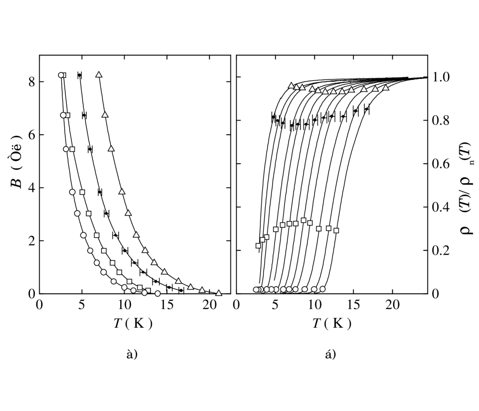
FIG. 2.: Characteristic points of the superconducting transition in sample 2a plotted in (a) $B$–$T$ and (b) $\rho$–$T$ planes (the resistivity is normalized to function $\rho_{n}(T)$ in Eq.(4), which was used in determination of the fluctuation conductivity): (open circles) ”irreversibility line”, $\rho=5$ $\mu\Omega$cm; (squares) peak of derivative $\partial\rho/\partial T$; (full circles) $B_{c2}(T)$; (triangles) ”transition onset” ${\partial\sigma_{fl}}/{\partial T}=10^{2}$ $\Omega^{-1}$cm${}^{-1}/$K.

In contrast to the case of optimal doping, the normal conductivity in our samples is low, of order of $e^{2}/\hbar d$ (Fig. 1), if $d$ is assumed to be of order of the lattice constant, 11.7 Å. Simple estimates based on the Aslamazov–Larkin formula (2) with a reasonable value of $d$ indicate that the contribution of fluctuations, $\sigma_{fl}$, should be several percent of $\sigma_{n}$ even at $\epsilon_{B}\gtrsim 0.5$. This makes determination of $\sigma_{n}(T)$ more difficult. The difficulties are exacerbated by the fact that the normal state resistivity has a minimum in the region of 30–40 K and increases at lower temperatures. Therefore, we decide to select a priori the function $\sigma_{n}(T)$ with several fitting parameters. The fitting to experimental data is performed by varying all parameters in both $\sigma_{fl}(T)$ and $\sigma_{n}(T)$.[29] This procedure could hardly produce sensible results if each curve $\rho(T)$ were described by a different set of parameters. Fortunately, the magnetoresistance of YBa₂Cu₃O_6+x crystals in the discussed region of fields and temperatures is negligible in the normal state, i.e., the shape of $\sigma_{n}(T)$ is constant with the magnetic field.

Our previous investigations of YBa₂Cu₃O_6+x single crystals near the boundary of the superconducting region of the phase diagram[32] revealed that the normal resistivity of such samples at $T<20$ K is well described by a logarithmic function. In a broader temperature range (0.5 K$<T<150$ K) the conductivity is very closely described by the empirical function

$$\sigma_{n}(T)=\rho_{n}^{-1}=[\alpha-\beta\log T+\gamma T]^{-1}$$ (4)

This function with three fitting parameters is used in processing our experimental data.

By approximating the conductivity in zero magnetic field by a sum of $\sigma_{n}(T)$ from Eq.(4) and $\sigma_{fl}(T)$ from Eq.(2), $T_{c}$ and $d$ being fitting parameters, along with $\alpha$, $\beta$ and $\gamma$, we obtain reasonable values $d=8$–15 Å, which are in fair agreement with the YBa₂Cu₃O_6+x lattice constant along the $c$-axis. This indicates that the Aslamazov–Larkin formula yields a correct estimate of the fluctuation conductivity in CuO₂ layers and its application is justified. The normal conductivity is fitted so as to obtain the best approximation of the fluctuation conductivity throughout the range of magnetic field. Nonetheless, the uncertainty in the normal resistivity was quite considerable. It turned out, however, that calculations of the transition temperature are little affected by admissible variations in $\sigma_{n}(T)$. The resulting uncertainties in the transition temperature are shown in Fig. 2.

This procedure enable us to derive $B_{c2}(T)$ in the mean–field approximation from our measurements. Since the resulting curve of $B_{c2}(T)$ is nonlinear and it casts doubt on the applicability of Eq.(3), we deem it necessary to demonstrate that, on the qualitative level, the shape of the $B_{c2}(T)$ curve is not affected by subtleties of the data processing, owing to the absence of considerable transition broadening. Figure 2a shows the curve of $B_{c2}(T)$ for sample 2a, along with its other characteristic fields, namely, the ”irreversibility line” determined at $\rho=5$ $\mu\Omega$cm, positions of the peak of derivative ${\partial\rho}/{\partial T}$, and the line of ”transition onset,” which was defined as a point were ${\partial\sigma_{fl}}/{\partial T}=10^{2}$ $\Omega^{-1}$cm${}^{-1}/$K. These lines are plotted in the $B$–$T$ diagram in Fig. 2a, and Fig. 2b shows positions of these points on the transition curves. (It is noteworthy that the values of $B_{c2}$ are fairly close to those which would be obtained by defining the transition point at a constant resistivity level $\rho/\rho{n}=0.8$.) Figure 2a clearly shows that all curves in the $B$–$T$ plane have positive curvature throughout the range of studied magnetic fields, including the region of low fields. This leads us to a conclusion that, even if the data processing procedure yields erroneous values of $B_{c2}$, the temperature dependence of this parameter is qualitatively correct. Our further analysis, however, will be based on the values derived from measurement data for the fluctuation conductivity.

C Universal temperature dependence of the upper critical field

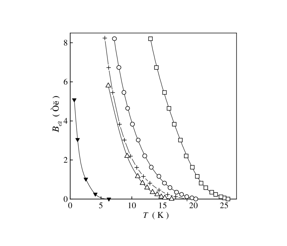
FIG. 3.: Temperature dependence $B_{c2}(T)$ in different states. Data for sample la in (empty triangles) quenched, (open circles) intermediate, and (squares) aged states; aged states of (crosses) sample 2a and (full inverted triangles) sample 3a.

Measurements of $B_{c2}(T)$ in three samples and five different states (all the states of samples la and 2a and the aged state of sample 3a) are given in Fig. 3. It turned out that the curves for all the states can be brought to coincidence by varying the scales of the magnetic field and temperature, i.e.,

$$B_{c2}=B_{sc}b_{sc}(t),\qquad t=\frac{T}{T_{c}},$$ (5)

where $B_{sc}$ is the parameter characterizing the state and $b_{sc}(t)$ is a universal function (Fig. 4). Function $b_{sc}(t)$ contains an arbitrary numerical factor. In Fig. 4 parameter $B_{sc}$ is defined as $B_{c2}$ at a specific reduced temperature equal for all samples, namely, $T_{c}/2$, i.e., the curves of $B_{c2}(T)$ were brought to coincidence at two points, namely, at $t=1$ and $t=0.5$. The values of $B_{sc}$ for different states are listed in Table I and plotted in the inset to Fig. 4 as a function of the zero-field transition temperature. These points lie on one smooth curve, even though they are derived from measurements of the three different samples. The characteristic scale of magnetic field decreases (accordingly, the coherence length increases) with decreasing doping level more rapidly than $T_{c}$, i.e., $B_{sc}$ is a superlinear function of $T_{c}$. This may be the main cause of the narrowing of the vortex-liquid region in the $B$–$T$ phase diagram. As a result, YBa₂Cu₃O_6+x crystals with a high degree of underdoping with $T_{c}\lesssim 30$ K do not display notable broadening of the resistive transition due to magnetic field.

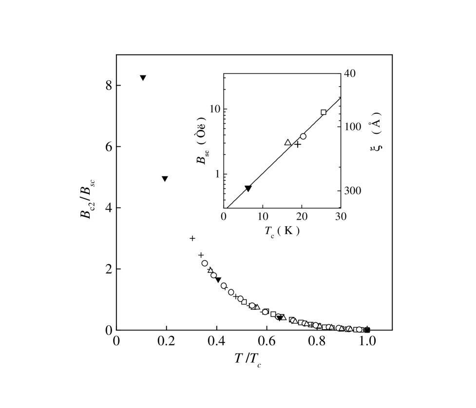
FIG. 4.: Dependencies $B_{c2}(T)$ for different samples reduced to the universal function $b_{sc}(t)$ using variables (5). The notation is the same as in Fig. 3. The inset plots the parameters $B_{sc}$ (left-hand axis) and correlation length $\xi_{0}$ calculated by Eq. 7 (right-hand axis).

The function $B_{c2}(T)$ was measured on sample 2b in a very narrow temperature range, $T/T_{c}\gtrsim 0.9$, owing to the limit on available magnetic fields. Its second derivative in this interval is also positive and all measurements of $B_{c2}(T)$ can be fitted to function (5). But, since no data for lower temperatures are available and the expected critical fields are very high, the measurements of sample 2b have not been analyzed in this context.

Function $b_{sc}(t)$ is much different from $b_{BCS}(t)$. First, it has no linear section near $t=1$. This statement relies on Eq. (5), since for each $B_{c2}(T)$ curve the limited precision allows one to draw a straight line of a small slope in the region within 1–2 K near $T_{c}$, but if we consider the samples with higher $T_{c}$, this linear region would be more narrow, and the slope of function $b_{sc}(t)$ at $t=$ is smaller, which leads us to a conclusion that the universal curve has no linear section near $t=1$.

Second, $b_{sc}$ continues to rise as $t\to 0$. Figure 4 shows this tendency in the region down to $t=0.1$. In order to test the range of lower $t$, we investigated sample 3b with $T\approx 3$ K at millikelvin temperatures. Its transition curve is too wide to determine quantitatively $T_{c}$ and $B_{c2}(T)$. Nonetheless, the measurements yield important qualitative information. Figure 5 shows the sample resistance versus magnetic field obtained at temperatures of 50 and 36 mK normalized to the resistance at a magnetic field of 14 T. It is clear that a drop in temperature shifts the magnetoresistance curve to lower fields, i.e., $B_{c2}(T)$ still grows with decreasing temperature even at $T/T_{c}\sim 0.01$. We can obtain the following estimate: on the level $\rho/\rho_{n}=0.8$, which approximately corresponds to $B_{c2}(T)$ according to Fig. 2b, the magnetic field increases by 0.6 T; this yields a derivative of 40 T/K. Unfortunately, we cannot plot these points in Fig. 4 for the lack of $T_{c}$ and $B_{sc}$.

FIG. 5.: Reduced resistivity of sample 3b in the aged state at temperatures of 50 and 36 mK as a function of magnetic field. The arrows indicate the difference between magnetic fields at which the curves cross the level $\rho/\rho_{14\,T}=0.8$.

This observation of $B_{c2}(T)$ increasing even at very low temperatures is in accord with measurements of other materials, e.g., Tl₂Ba₂CuO₆,[2] where the upper critical field continues to grow at temperatures down to $T/T_{c}=0.001$.

Our data indicate that function $B_{c2}(T)$ in underdoped YBa₂Cu₃O_6+x is nonlinear in the neighborhood of $T_{c}$, and $(\partial B/\partial T)|_{T_{c}}=0$. This conclusion contradicts most theoretical models based on the BCS model or the Ginzburg–Landau functional, which either predict a linear behavior of this curve near $T_{c}$ or assume its existence a priori. This issue was not discussed in previous publications of experimental investigations,[2, 3, 4, 5, 6, 7] but they all reported very low, if not zero, values of $(\partial B/\partial T)$ at $T_{c}$.

The increase in the critical field owing to weakening of the spin-flip scattering predicted by Ovchinnikov and Kresin[8] should occur in the range of low temperatures, so it leaves the linearity of $B_{c2}(T)$ near $T_{c}$. essentially unaffected. The mechanism suggested by Spivak and Zhou[9] is effective only in high magnetic fields, where Landau quantization is significant, i.e., it also should not affect $B_{c2}(T)$ near $T_{c}$. Abrikoso[11] derived $B_{c2}(T)$ from the Ginzburg–Landau functional based on his model, which leads, naturally, to a linear dependence of $B_{c2}$ in the first order in $1-t$.

The nonlinearity of $B_{c2}(T)$ near $T_{c}$ follows at present only from the model of bipolaron superconductivity[10, 33] which yields positive curvature of $B_{c2}(T)$ for a charged Bose-liquid in a localizing potential, this throughout the entire temperature range. At temperatures that are not overly low, the model predicts[33]

$$B_{c2}(T)=B_{d}^{*}\left(\frac{T_{c}}{T}\right)^{3/2}\left[1-\left(\frac{T}{T_{c}}\right)^{3/2}\right]^{3/2},$$ (6)

$$\quad B_{d}^{*}=\frac{\Phi_{0}}{2\pi\xi_{0}^{2}}\left(1-\frac{n_{L}}{2n}\right)^{1/2}$$ (7)

Here $\xi_{0}$ is the correlation length and $n_{L}/2n$ characterizes the random potential. Equation (7) defines a universal function in reduced variables without free parameters. The only normalization parameter $B^{*}_{d}$ corresponds to parameter $B_{sc}$ introduced in Eq. (5). It follows from Eq. (7) that $B^{*}_{d}=0.68B_{sc}$. Comparison between our data and calculations by Eq. (7) (Fig. 6a) shows excellent agreement in the region $T/T_{c}>0.3$. At lower reduced temperatures experimental points deviate from the theoretical curve, but note that in this range we have only measurements of one state (sample 3a aged).

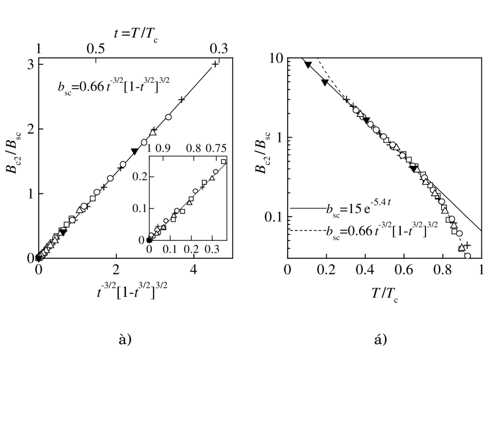
FIG. 6.: Function $b_{sc}(t)$ plotted in different coordinates: (a) the coordinates are selected in accordance with the boson model, Eq. (7); the inset shows the section close to $t=T/T_{c}=1$ on the extended scale; (b) semilogarilhmic coordinates; the dashed line follows Eq. (7).

The factor $(1-n_{L}/2n)^{1/2}$ in Eq. (7) is unknown, but, since neither in state 3a nor in state 3b have we detected a reentrant behavior of $B_{c2}(T)$ predicted by Alexandrov,[33] it should be rather close to unity. Assuming this, we can derive from Eq. (7) the correlation length $\xi_{0}$ (Fig. 4, right-hand axis in the inset). The length $\xi_{0}$ varies between 70 and 300 Å. The notable increase in the correlation length may be the main cause of the narrowing of the vortex liquid region on the $B$–$T$ diagram.

In the low-temperature region $0.1<t<0.6$ the function $b_{sc}(t)$ can be empirically described by the exponential

$$b_{sc}=b_{0}\exp(-t/t_{0})$$ (8)

with parameters $b_{0}=15$ and $t_{0}=5.4$ (Fig. 6b). Such an unusual temperature dependence in the region of low temperatures was detected previously[25, 34] in measurements of the irreversibility line $B^{*}(T)$. We suppose that the region of vortex liquid in phase diagrams of samples with low $T_{c}$ is a very narrow strip between $B^{*}$ and $B_{c2}$, hence $B^{*}$ closely follows $B_{c2}(T)$, especially at low temperatures.

V Conclusions

Our investigation has supplemented the list of materials displaying anomalous temperature dependence of the upper critical field $B_{c2}(T)$ with underdoped cuprate YBa₂Cu₃O_6+x. We have studied samples with different carrier concentrations and $T_{c}$ ranging between 6 and 30 K. Throughout the studied temperature range, the curve of $B_{c2}(T)$ for these samples have positive curvature and does not saturate at low temperatures. The curves for states with different $T_{c}$ can be brought to coincidence in reduced coordinates $T/T_{c}$ and $B/B_{sc}(T_{c})$. A fundamental feature of the universal function $b_{sc}(t)$ obtained in this manner is the tendency of its first derivative $\partial B_{c2}/\partial T$ to zero as $T\to T_{c}$. Such a behavior can be interpreted at present only in terms of the model[10, 33] treating the superconducting transition as Bose-condensation of preformed pairs. Other models designed to interpret the anomalous shape of the $B_{c2}(T)$ curve predict a linear temperature dependence of $B_{c2}$ near $T_{c}$.

In the low-temperature range $T/T_{c}<0.3$, experimental points deviate from function (7). On the other hand, measurements in the temperature interval between the lowest accessible values and $t\approx 0.6$ follow function (8). The combination of Eqs. (7) and (8) analytically describes function $b_{sc}(t)$.

However, the ”universality” of function $b_{sc}(t)$ is limited. We tested this function on our measurements of K_0.4Ba_0.6BiO₃,[5] and the experimental curve after renormalization of variables according to Eq. (5) was different from function $b_{sc}(t)$ plotted in Fig. 4.

We are indebted to V.T. Dolgopolov and A.A. Shashkin for the opportunity to conduct low-temperature measurements in the dilution refrigerator.

This work was supported by RFBR-PICS (Grant 98-02-22037), by RFBR-INTAS (Grant 95-02-302), and by the Statistical Physics Program sponsored by the Russian Ministry of Science and Technology.

REFERENCES

- [1] N.R. Werthamer, E. Helfand, and C. Hohenberg, Phys. Rev. 147, 295 (1966).
- [2] A.P. Mackenzie, S.R. Julian, G.G. Lonzarich et. al., Phys. Rev. Lett. 71, 1238 (1993).
- [3] M.S. Osofsky, R.J. Soulen, Jr., S.A. Wolf et. al., Phys. Rev. Lett. 71, 2315 (1993).
- [4] M. Affronte, J. Marcus, C. Escribe-Filippine et. al., Phys. Rev. B 49, 3502 (1994).
- [5] V. F. Gantmakher, L. A. Klinkova, N. V. Barkovskii et. al., Phys. Rev. B 54, 6133 (1996).
- [6] D. D. Lawrie, J. P. Franck, J. R. Beamish et. al.. J. Low Temp. Phys. 107, 491 (1997).
- [7] Y. Dalichaouch, B. W. Lee, C. L. Seaman, J. T. Markert, and M. B. Maple, Phys. Rev. Lett. 64, 599 (1990).
- [8] Yu. N. Ovchinnikov and V. Z. Kresin. Phys. Rev. B 54, 1251 (1996).
- [9] B. Spivak and Fei Zhou, Phys. Rev. Lett. 74, 2800 (1995).
- [10] A. S. Alexandrov and N. F. Mott, Rep. Prog. Phys. 57, 1197 (1994).
- [11] A. A. Abrikosov, Phys. Rev. B 56, 446, 5112 (1997).
- [12] A. S. Alexandrov, V. N. Zavaritsky, W. Y. Liang, and P. V. Nevsky, Phys. Rev. Lett. 76, 983 (1996).
- [13] A. V. Nikulov, Phys. Rev. Lett. 78, 981 (1997).
- [14] D. S. Fisher, M. P. A. Fisher, and D. A. Huse, Phys. Rev. 43, 130 (1991).
- [15] G. Blalter, M. V. Feigelman, V. B. Geshkenbein, A. I. Larkin, and V. M. Vinokur, Rev. Mod. Phys. 66, 1125 (1994).
- [16] S. Ullah and A. T. Dorsey, Phys. Rev. B 44, 262 (1991).
- [17] M. Tinkham, Phys. Rev. Lett. 61, 1658 (1988).
- [18] M. Suzuki and M. Hikita, Phys. Rev. B 44, 249 (1991).
- [19] A. Carrington. D. J. C. Walker, A. P. Mackenzie, and J. R. Cooper, Phys. Rev. B 48, 13051 (1993).
- [20] S. Fleshier, W. K. Kwok, U. Welp et. al.IEEE Trans. Appl. Supercond. 3, 1483 (1993).
- [21] G. W. Crabtree and D. R. Nelson, Phys. Today 4, 38 (1997).
- [22] A. Camngton, A. P. Mackenzie, and A. Tyier, Phys. Rev. B 54, R3788 (1996).
- [23] W. K. Kwok, S. Fleshier, U. Welp et. al., Phys. Rev. Lett. 69, 3370 (1992).
- [24] A. N. Lavrov and L. P. Kozeeva, Physica C 248, 365 (1995).
- [25] G. T. Seidler, T. F. Rosenbaum, D. L. Beinz et. al.. Physica C 183, 333 (1991).
- [26] A. N. Lavrov and L. P. Kozeeva, Physica C 253, 313 (1995).
- [27] S. I. Dorozhkin, G. V. Merzlyakov, and V. N. Zverev, Prib. Tekh. Eksp. No. 2. 165 (1996).
- [28] T. A. Friedmann, J. P. Rice, J. Giapintzakis, and D. M. Ginsberg, Physica C 39, 4258 (1989).
- [29] S. B. Han, C. C. Almasan, M. C. de Andrade et at., Phys. Rev. B 46, 14290 (1992).
- [30] M. A. Crusellas, J. Fontcuberta, and S. Pinol, Physica C 213, 403 (1993).
- [31] B. Iwasaki, S. Inaba, K. Sugioka et. al., Physica C 290, 113 (1997).
- [32] V. F. Gantmakher, L. P. Kozeeva, A. N. Lavrov et. al., JETP Lett. 65, 870 (1997).
- [33] A. S. Alexandrov, Phys. Rev. B 48, 10571 (1993).
- [34] K. E. Gray. D. B. Kim, B. W. Veal et. al.. Phys. Rev. B 45, 10071 (1992).