Domain-Wall Free-Energy of Spin Glass Models :
NumericalMethod and Boundary Conditions

Abstract

An efficient Monte Carlo method is extended to evaluate directly domain-wall free-energy for randomly frustrated spin systems. Using the method, critical phenomena of spin-glass phase transition is investigated in $4d\pm J$ Ising model under the replica boundary condition. Our values of the critical temperature and exponent, obtained by finite-size scaling, are in good agreement with those of the standard MC and the series expansion studies. In addition, two exponents, the stiffness exponent and the fractal dimension of the domain wall, which characterize the ordered phase, are obtained. The latter value is larger than $d-1$, indicating that the domain wall is really rough in the $4d$ Ising spin glass phase.

]

I Introduction

Numerical simulations, in particular Monte Carlo (MC) methods, have played a quite important role in spin glass (SG) studies[1]. For example, very large-scale MC simulations have strongly suggested the existence of a SG phase transition in three-dimensional Ising SG systems.[2, 3, 4] In these studies, a cumulant of SG overlap function $q$, so called the Binder parameter, has frequently used in order to extract critical temperature $T_{\rm c}$. However, the Binder parameter in $3d$ Edwards-Anderson (EA) Ising models[4, 5] merely depends on system sizes below $T_{\rm c}$ as compared to that above $T_{\rm c}$[6]. Moreover, unusual size dependence of the Binder parameter is observed in short-ranged Ising EA model under the magnetic field[7]. Consequently, the existence of the SG phase transition under the field has still remained unclear. In order to settle the issue and make a progress toward well-understanding of SG picture, we consider other numerical analyzes to be quite necessary.

In this direction, some promising ways have recently been proposed based on non-equilibrium dynamics[8, 9] and the idea of non-self-averaging[10], but here we pay attention to domain-wall renormalization group method (DWRG) originally proposed by McMillan[11]. The DWRG estimates a singular part of free energy by calculating the domain-wall free energy, $\Delta F$, which is defined as the free-energy difference between periodic- and anti-periodic boundary conditions (BC). In the scaling regime at low temperatures, $\Delta F$ follows a power law as a function of the system size $L$, $\Delta F\sim L^{\theta}$, where the stiffness exponent $\theta$ is related to the rigidity of the system. If the exponent $\theta$ takes a positive value at a temperature, then the system stays in an ordered phase. On the other hand, a negative exponent means a disordered phase. In this sense, the sign of the exponent $\theta$ is an indicator of the existence of long range ordering. This exponent $\theta$ also characterizes a low-energy excitation in the SG phase and is predicted to be smaller than $(d-1)/2$, $d$ being dimensionality, in the droplet scaling theory[12, 13].

The DWRG approach relies on an accurate way for estimating the free-energy difference between two BCs. It is a difficult task in general for MC method to estimate free energy or entropy. Except for the numerical transfer matrix method for Ising models, it is therefore usual to integrate over the free-energy derivative, measured by MC simulations, along a parameter path between a reference system and the one of interest. As for zero-temperature calculations, various optimization techniques have been demonstrated to be useful for Ising[14, 15] and vector spin systems[16]. These facts restrict so far to rather small sizes and/or at zero temperature. In this work we have developed a boundary-flip MC method proposed by Hasenbusch[17] which allows us to estimate free-energy difference at a finite temperature directly from MC simulation. In applying a naive boundary-flip MC method to large systems and/or at low temperatures, one may encounter a hardly relaxing problem even in simple models without many meta-stable states, namely the system is trapped into a local area in the phase space. The original work[17] has successfully overcome the relaxational problem by combining the method with the cluster MC dynamics.

In the present paper, we have proposed an alternative strategy, which is the boundary-flip method with exchange MC (EMC) method[18], in order to make the relaxation faster. This combined method is found to be quit efficient for randomly frustrated spin systems such as spin glasses, while the original method based on the cluster MC method is restricted to non-frustrated systems. The present method is applicable to a wide class of spin systems. Moreover, the direct measurements have an advantage over the thermodynamic integration method from a numerical standpoint, because statistical error is controlled within MC scheme in the former. Consequently, we have succeeded to estimate the free-energy difference in a SG model, accurately enough to observe systematic correction to finite-size scaling.

For applying DWRG to SG systems, we need to choose the relevant boundary conditions to the ordered phase. The standard approach has often used a randomly fixed spin boundary condition[19]. Instead, we employ the replica boundary condition proposed by Ozeki[25], in which two real replicas are coupled with each other through a boundary surface. The replica boundary condition provides that the domain-wall free energy becomes positive at any bond disorder, implying that it is conjugates to the SG ordering. This positivity is of benefit to us for estimating the domain-wall free energy accurately from a numerical point of view.

Here we study the $4d\pm J$ Ising SG model under the replica BC by the novel MC method. We obtain the critical temperature and the exponent by finite-size-scaling analysis of the domain-wall free energy, in agreement with the previous works. In addition, we estimate two exponents, the stiffness exponent $\theta$ and the fractal dimension $d_{s}$ of the domain wall. We find that $d_{s}$ is larger than $d-1$ in the SG phase.

This paper is organized as follows: In the next section, we explain the method for calculating the domain-wall free energy. Section III is mainly devoted to discussion about the replica boundary conditions. We give an interpretation of domain wall appearing in the replica boundary condition and propose a way to measure the morphology of the domain wall. We show results for application of the method to $4d\pm J$ Ising SG model in the section IV. In the last section, possible extensions of the method and nature of the low-temperature phase are discussed. Appendix A contains a way for setting temperature points which is needed before simulation in the exchange MC method.

II Boundary flip MC method with exchange process

In this section we describe a method that allows us to evaluate directly the domain-wall free-energy using MC simulations. For the sake of simplicity, we restrict ourselves to Ising spin systems and fixed spin boundary conditions. Let us consider a total model Hamiltonian defined by

$${\cal H}_{\rm tot}(\sigma,S_{1},S_{2})={\cal H}_{\rm model}(\sigma)+\alpha{\cal H}_{\rm BC}(\sigma,S_{1},S_{2}),$$ (1)

where $\sigma$ denotes Ising spin variable defined on a $d$-dimensional hyper-cubic lattice $V$ of $L^{d}$ and two additional spins $S_{1}$ and $S_{2}$ represent boundary spins. The second term gives a coupling between the model system and the boundary spins along one direction as

$${\cal H}_{\rm BC}(\sigma,S_{1},S_{2})=-\sum_{i\in\partial_{1}V}J_{i,1}\sigma_{i}S_{1}-\sum_{i\in\partial_{2}V}J_{i,2}\sigma_{i}S_{2},$$ (2)

where the summation runs over one surface $\partial_{1}V$ of the lattice $V$ and its opposite surface $\partial_{2}V$. A standard periodic boundary condition for $\sigma$ is used along the remaining directions. Then the total partition function $Z_{\rm tot}$ and the free energy $F_{\rm tot}$ of this whole system are defined by

$$Z_{\rm tot}(T) = {\rm Tr}_{\{\sigma,S_{1},S_{2}\}}\exp(-H_{\rm tot}(\sigma,S_{1},S_{2})/T)$$ (3)

$$= \exp(-F_{\rm tot}(T)/T),$$ (4)

where $T$ is temperature and we set the Boltzmann constant to unity. The phase space of the total Hamiltonian is enlarged by adding the degree of freedom of the boundary spins $S_{1}$ and $S_{2}$. When these spins are in parallel, the boundary condition is regarded as periodic and similarly the anti-periodic boundary condition corresponds to anti-parallel boundary spins. For a given temperature the probability for finding the periodic boundary condition is given by

$$P_{\rm P}(T) \equiv \frac{{\rm Tr}_{\{\sigma,S_{1},S_{2}\}}\delta_{S_{1},S_{2}}\exp(-{\cal H}_{\rm tot}(\sigma,S_{1},S_{2})/T)}{Z_{\rm tot}(T)},$$ (5)

$$= \frac{Z_{\rm P}(T)}{Z_{\rm tot}(T)},$$ (6)

where $\delta$ is the Kroneker delta function. This quantity is accessible from MC simulation, namely it is nothing but the probability for realizing the periodic BC during MC simulation in which the boundary spins as well as the bulk spins are updated according to a standard MC procedure. In terms of the probability and the corresponding one to the antiperiodic BC, domain-wall free-energy $\Delta F$ we want to investigate is given by

$$\exp(\beta\Delta F(T))=e^{-\beta(F_{\rm P}-F_{\rm AP})}=\frac{Z_{\rm P}}{Z_{\rm AP}}=\frac{P_{\rm P}(T)}{P_{\rm AP}(T)}.$$ (7)

This is the basic idea of the boundary flip MC method proposed by Hasenbusch[17]. When we adopt a naive local updating process for the boundary spins in the boundary-flip MC method, however, we are at once faced to a hardly relaxing problem. For example, once the anti-periodic boundary conditions and the domain-wall structure in the system are realized in the simulation at low temperatures, as shown in Fig. 1, the boundary spins are kept to be fixed in the sense that the probability for flipping these spins is vanishing in practice. This fact makes statistical error of $\Delta F$ significantly large. The original work[17] has overcome this difficulty by utilizing the modified cluster flip. We can also practically solve this so-called hardly relaxing problem using recently proposed extended ensemble methods such as the multicanonical MC method[20], the simulated tempering[21] and the exchange MC method[18]. In fact, a similar difficulty has been overcome using the multicanonical idea in the lattice-switch MC method[24], which has been proposed to estimate the free-energy difference between two different crystalline structure in a hard sphere system.

FIG. 1.: Typical example for metastable configuration in a ferromagnetic model.

In the present work, we employ the exchange MC method (EMC) in order to obtain an efficient path between two boundary-condition states. In the EMC method, we simulate a combined system which consists of non-interacting $M$ replicated system. The $m$-th replica is simulated independently with its own external variable such as temperature. We introduce exchange process between configurations of two of $M$ replicas with the whole combined system remaining in equilibrium. One possible way for obtaining the path is that we distribute various values of the coupling $\alpha$ in eq. (1) ranging from 0 to 1 to $M$ replicas. A target system we are physically interested in is the replica with $\alpha=1$. For a replica with null coupling of $\alpha$, which we call a source system, the boundary spins can be flipped freely. Therefore, the path between different boundary condition states in the target system would be recovered by the exchange process through the source system.

FIG. 2.: Schematic picture of the exchange line in parameter space.

In randomly frustrated spin systems such as SG models, there is another serious relaxation problem arising from bulk spins in the model system itself. This problem can be overcome also by the EMC method.[18] When we distribute $M$ temperature points widely including high enough temperature in a disordered phase, configurations at low temperatures are expected to be refreshed through the exchange process. The EMC method has turned out to work efficiently in the SG systems[18, 22]. Therefore, for the boundary-flip MC method on SG models, we need to construct the EMC method in two-dimensional parameter space of the coupling $\alpha$ and the temperature $T$. It is possible to introduce the exchange process in the two parameter space, but it is quite time consuming. In the present work, therefore, we choose an exchange line in the two dimensional space appropriately, namely we set a system at high temperature with $\alpha=0$ as one end of the exchange line and systems at lower temperature with $\alpha$ being unity, as shown in Fig. 2. It is noted that the parameter region of the our final interest lies on the line with $\alpha=1$ around $T_{\rm c}$ and below. An efficient choice of the exchange line would depend on systems we want to investigate. Actual implementation to the Ising spin glass model will be explained in detail in Section IV.

III Replica Boundary Conditions for SG systems

In this section, we discuss how to choose boundary condition for SG systems in the DWRG study. We concentrate ourselves on a way of choice of boundary condition along one direction while the remaining ones are considered to be given appropriately. In a conventional DWRG studies[11, 23] as well as the defect energy method, a boundary condition frequently used is a connected spin BC in which the corresponding boundary term in eq. (1) is described by

$${\cal H}_{\rm BC}=\sum_{i\in\partial_{1}V,j\in\partial_{2}V}J_{ij}\sigma_{i}\sigma_{j}.$$ (8)

The case with $\alpha/|\alpha|=1(-1)$ is regarded as the (anti-) periodic boundary condition. For the boundary condition defined by eq. (8), the boundary-flip MC method can be applied by treating the sign of the coupling $\alpha$ as a MC dynamical variable. In SG systems, the free-energy difference between these BCs cannot be assured positive so that the width of distribution of the free-energy difference is examined as an effective coupling of the SG ordering, $F_{\rm eff}=\sqrt{(F_{\rm AP}-F_{\rm P})^{2}}$. To evaluate the mean width is rather difficult as compared with the average in numerical calculations. Further, it is less clear how the domain wall is created in a random spin system under these BCs.

In order to avoid the difficulty and make clear an idea of the domain wall, Ozeki[25] has proposed a replica boundary condition (RBC), in which two real replicas are prepared with the same bond realization. Its essential point is to introduce a uniform coupling between these two replicas only for one surface $\partial_{0}V$ along a given direction. For the other directions periodic BC is employed as usual. We show explicitly an example expressed as the Ising Hamiltonian

$${\cal H}_{\rm model}(\sigma,\tau)=-\sum_{\langle ij\rangle}J_{ij}(\sigma_{i}\sigma_{j}+\tau_{i}\tau_{j})-J_{\rm int}\sum_{i\in\partial_{0}V}\sigma_{i}\tau_{i},$$ (9)

where both $\sigma$ and $\tau$ are Ising variables and the summation of the first term runs over nearest neighbor bonds. The second term corresponds to the replica interaction mentioned above. When $J_{\rm int}$ is set to (anti-) ferromagnetic, the boundary condition is called replica (anti-) periodic, R(A)PBC. Spins on the opposite side of $\partial_{0}V$ are kept randomly fixed with $\sigma_{i}=\tau_{i}$.

Ferromagnetic interactions between the replicas in the RPBC prefer a self-overlap state, even if the system has many local minima or pure states. Namely, one replica gives an effective conjugated field to the other replica through the inter-replica interaction. It is convenient to consider the domain wall in terms of the replica overlap $q_{i}=\sigma_{i}\tau_{i}$. The self-overlap state is characterized by positive values of $q_{i}$ at all the sites, meaning no domain wall in the system. At sites on the opposite surfaces of $\partial_{0}V$, $q_{i}$ take unity by definition, irrespective of R(A)PBCs. On the other hand, anti-ferromagnetic inter-couplings between the replicas in the RAPBC would induce negative overlap at sites near the coupling. Therefore, at least one domain wall, characterized by a region where the sign of $q_{i}$ changes, likely appears in the RAPBC, if the system has a rigid ordered state. From a mathematical point of view, non-negativity of the free-energy difference $\Delta F_{\rm R}=F_{\rm RAPBC}-F_{\rm RPBC}$ under the replica BC has been proven rigorously in any random Ising model at any finite temperature using the transfer matrix formalism[25]. This non-negativity holds true irrespectively of a choice of spins on the surface opposite to $\partial_{0}V$. As a result, only average of the domain-wall free energy is needed for estimating an relevant effective coupling of the SG ordering. This is advantageous for reducing statistical error of $\Delta F_{\rm R}$ from which a transition point from paramagnetic to SG phase is detected.

An additional merit of the replica boundary condition is that we can discuss the morphology of the domain wall at finite temperatures. In terms of the local overlap $q_{i}$, the area of the domain boundary mentioned above is expressed as $W=\sum_{\langle ij\rangle}\frac{1}{2}(1-q_{i}q_{j})$, where the summation is over nearest-neighboring pairs. . Then we can extract directly domain-wall properties such as its fractal dimension, from the difference $\Delta W(T)$ defined by

$$\Delta W(T)=\frac{1}{2}\sum_{\langle ij\rangle}(\langle\sigma_{i}\sigma_{j}\tau_{i}\tau_{j}\rangle_{\rm RPBC}-\langle\sigma_{i}\sigma_{j}\tau_{i}\tau_{j}\rangle_{\rm RAPBC}),$$ (10)

where $\langle\cdots\rangle_{\rm R(A)PBC}$ denotes the thermal average under the replica (anti-) periodic BC. This quantity is also regarded as a difference of link correlation[26] between two boundary conditions in $\pm J$ models. The correlation function as well as the replica overlap have been studied in a similar replicated system[26] which has a global coupling between the replicas. This coupled system is different from the present system under RBC. In particular, the correlation function (10) is related to domain-wall properties only in the RBC. The domain-wall area $\Delta W$ has not been directly studied so far in SG systems, except for the zero temperature calculation in two dimensional Ising SG model[33]. We will present new results for $\Delta W$ in the next section.

IV results

In this section, we present results of an application of the novel MC method explained in the previous sections to $4d\pm J$ Ising SG model. The interactions $\{J_{ij}\}$ in eq. (9) are random variables which take values $\pm J$ with equal probability. The boundary-flip MC method can be applied to the replica BC by regarding the sign of the interaction $J_{\rm int}$ in eq. (9) as a dynamical variable. Equivalently these boundary conditions are defined by relative direction of the boundary spins $S_{1}$ and $S_{2}$ added to eq. (9) whose $J_{\rm int}$ are fixed to be positive. Then, the boundary part in eq. (1) is given by

$${\cal H}_{\rm BC}(\sigma,\tau,S_{1},S_{2})=-\sum_{i\in\partial V}J_{i}(\sigma_{i}S_{1}+\tau_{i}S_{2}),$$ (11)

where the interactions $J_{i}$ are also distributed randomly. In the present work we adopt this method with the boundary spins.

The number of the replicas $M$ in the EMC method is fixed $32$ irrespectively of the system sizes to utilize the multi-spin coding technique. Each replica with the parameters $\alpha$ and $T$ tries to exchange configuration with the nearest replica in the parameter space. As we have explained in Section II, we choose in this two-parameter space, a line on which $M$ replicas are prepared. The line chosen is such that value of $\alpha$ is unity below a certain temperature $T_{m}$, but it decreases like a Gaussian formula as a function of $T-T_{m}$ above $T_{m}$. The onset $T_{m}$ is set to be about 2 times of the critical temperature. We distribute the set of the parameters to the 32 replicas such that the acceptance ratio for each exchange process becomes independent of the replicas. This can be succeeded by a simple iteration method using the energy function, which is estimated from a short preliminary run. Details of the iteration method is explained in Appendix.

As an equilibration check, we study time evolution of $\Delta F_{\rm R}$ starting from two initial conditions: periodic and anti-periodic boundary conditions imposed for the whole replicated systems in the EMC simulation. The initial conditions for the bulk spins are chosen at random. The free-energy difference $\Delta F_{\rm R}$ is estimated as a function of MC step $t$ by averaging over short MC steps around the time $t$. In the case of the whole anti-periodic BC, free-energy difference, starting from a large negative value at the initial time, evolves toward equilibrium. The other estimation with the periodic BC at the initial time reaches to the equilibrium value from the opposite direction to that of the anti-periodic BC. In equilibrium, two curves coincide with each other. As expected, we see in Fig. 3 that the equilibration of $\Delta F_{\rm R}$ is obtained after a certain time. It should be noted that the relaxational function approaching to the equilibrium value follows an exponential law rather than a power law observed in the standard SG simulations. This implies the existence of a typical time scale for equilibration in the present method. We thus expect that the system really reaches equilibrium after a few times of such time scale. We estimated the time scale for other sizes and determined the MC steps (MCS) for thermalization and measurements. For example, in simulations of $4d$ case with $L=8$, we take $9.6\times 10^{4}$ MCS for the initial step and $2.0\times 10^{5}$ MCS for measurement. We have also checked that the ergodic time[20, 18] is about $3\times 10^{2}$, $3.0\times 10^{4}$, $5.8\times 10^{4}$ and $1.7\times 10^{5}$ MCS on average for $L=4,6,8,$ and $10$, respectively.

FIG. 3.: The domain-wall free-energy of $4d\pm J$ Ising SG model with $L=8$ and $T=1.694$ well below the SG transition temperature as a function of MC steps. The upper data marked by open triangle are started from the periodic boundary condition for the whole system, while the lower one from the anti-periodic one. Each point at the time $t$ is obtained by averaging over 2,000 MCS around $t$ and error bars are estimated from statistical fluctuation over 10 samples.

We show temperature dependence of $\Delta F_{\rm R}$ for the $4d$ Ising SG model in Fig. 4. The lattice size studied are $L=4,6,8,$ and $10$ with samples 2197, 2060, 1332, and 892, respectively. According to the standard finite-size-scaling argument, the domain-wall free energy should be scaled as

$$\Delta F_{\rm R}(L,T)\sim F_{0}((T-T_{\rm c})L^{1/\nu}),$$ (12)

where the parameter $\nu$ denotes the critical exponent of the correlation length and $F_{0}$ is a scaling function. Therefore, the critical temperature can be located in the point where $\Delta F_{\rm R}$ for different sizes as a function of $T$ cross with each others. The crossing feature of $\Delta F_{\rm R}$ at $T_{\rm c}$ is common to the Binder parameter. In fact, as shown in Fig. 4, crossing of $\Delta F_{\rm R}$ of two different sizes is seen at a certain temperature. However the crossing temperature is found to shift systematically to low temperature side as the system size increases, implying that correction to the finite-size scaling is significant. We consider correction due to the leading irrelevant scaling variable whose scaling dimension is $\omega$;

$$\Delta F_{\rm R}(L,T)\sim F_{0}((T-T_{\rm c})L^{1/\nu})+L^{-\omega}F_{1}((T-T_{\rm c})L^{1/\nu}),$$ (13)

These exponent $\nu$ and $\omega$ and the critical temperature $T_{c}$ are determined by fitting the simulated data to the scaling formula (13), where the scaling functions $F_{0}$ and $F_{1}$ are assumed to be given by third order polynomial functions. From the fitting, we estimate $T_{\rm c}=2.00(4)$, $\nu=0.92(6)$, and $\omega=1.5(9)$. The finite size scaling of $F_{0}$ after subtraction of the leading correction is plotted in Fig 5, where all the data points are found to collapse almost into a universal function. The scaling plot including the smallest size $L=4$ is obtained only when the leading term of the correction is taken into account. The estimated critical temperature is consistent with the previous results obtained by the MC method[27] and the high temperature expansion[29, 30]. Our result for $\nu$ is also in agreement with these expansion studies, and not very different with that obtained by MC simulations for $\pm J$[27] and Gaussian distribution[28]. Since the system sizes used in the present work are larger than those in the previous MC simulations, we expect that our estimation is reliable. The irrelevant exponent $\omega$ is, to our knowledge, the first estimation for $4d$ Ising SG model by MC simulation, but its value is slightly lower than that obtained from the series expansion[30] that quoted about 3.

FIG. 4.: Temperature dependence of the domain-wall free-energy for $4d$ $\pm J$ Ising SG model near the critical temperature. These lines are for guide of eyes.

At low enough temperature, the domain-wall free energy is expected to be scaled as

$$\Delta F_{\rm R}(L,T)\sim L^{\theta},$$ (14)

where $\theta$ is an exponent which gives the characteristic energy scale $L^{\theta}$ of low energy excitations of typical size $L$. We cannot evaluate $\Delta F_{\rm R}$ at low temperatures enough to distinguish the low temperature properties from the critical behavior. Here we try to estimate the exponent $\theta$ from the scaling function of $\Delta F_{\rm R}$. We assume that the behavior of $\Delta F_{\rm R}$ at a large length scale is also described by the scaling form of eq. (13) near below $T_{\rm c}$. This assumption implies that the asymptotic behavior of the scaling function $F_{0}$ is predicted as

$$F_{0}(x)\sim|x|^{\theta\nu},$$ (15)

at $x\rightarrow-\infty$. We examine this scaling idea in the simple $3d$ Ising ferromagnetic model, where the stiffness exponent coincides with the surface dimensions $d-1$. We estimate the domain-wall free energy by the present MC method under the connected spin BC described in (8). In the $3d$ Ising model, we scale the data to the leading scaling formula (12) without the correction, because we have not observed a shift of the crossing temperature under our numerical accuracy. The finite-size scaling of the domain-wall free energy works well as observed in Fig. 6. The asymptotic behavior of the scaling function gives $\theta\nu\sim 1.27$, compatible with the well-known values of $\nu$ and $\theta=d-1$.

FIG. 5.: Finite-size scaling plot of the domain-wall free energy in $4d\pm J$ Ising SG model. The leading correction to the scaling is taken into account. The scaling plot after subtraction of the leading correction is shown. The estimated scaling parameters are $T_{c}=2.00(4)$, $\nu=0.92(6)$ and the irrelevant exponent $\omega=1.5(9)$. The slope of the scaling function is asymptotically close to $0.75(1)$, meaning that the stiffness exponent $\theta$ is $0.82(6)$.

Let us turn to the $4d$ Ising SG model. The stiffness exponent $\theta$ in SG systems is expected much smaller than that of the ferromagnetic model. The droplet theory predicted the upper bound of $\theta$ to be $(d-1)/2$[13]. We extract value of $\theta$ from the scaling function obtained in Fig. 5. We fit the scaled data with the scaling variable $x$ larger than 3 to a power law. The best fit is obtained with the exponent $\theta\nu=0.75(1)$, which yields the stiffness exponent of $\theta=0.82(6)$.

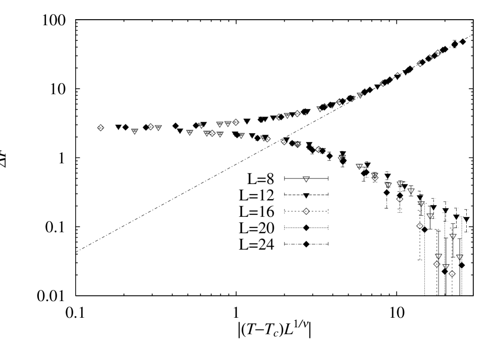
FIG. 6.: Finite size scaling plot of the domain-wall free energy in $3d$ ferromagnetic Ising model. The parameters of the scaling are estimated as follows: $T_{c}=4.5117(4)$, $\nu=0.624(7)$. The asymptotic behavior of the scaling function follows a power law as a function of the scaling parameter $(T-T_{c})L^{1/\nu}$ with slope $1.27(1)$. The value of the slope is compatible with the low temperature behavior, namely $\theta\nu$, being $\theta=d-1$.

We also investigate the domain-wall area $\Delta W$ defined by eq. (10) in this model, which is easily calculated in the present MC scheme. A scaling analysis similar to the one for $\Delta F_{\rm R}$ is performed for $\Delta W$, taking into account the leading correction to the scaling. It is noted that in contrast with the $\Delta F_{\rm R}$ scaling, $\Delta W$ is proportional to $L^{2/\nu}$ near $T_{\rm c}$ because it has essentially the same scaling dimension as the energy-energy correlation function. The finite-size-scaling plot for $\Delta W$ is shown in Fig. 7, where the critical temperature is used which is estimated by the $\Delta F_{\rm R}$ scaling. The scaling nicely works both above and below $T_{\rm c}$ and the estimated $\nu$ value is consistent with that from $\Delta F_{\rm R}$. We suppose that at low temperature the domain wall in the SG system is rather rough. Correspondingly the domain-wall area $\Delta W$ is expected to follow a power law on size with a non trivial fractal dimension $d_{s}$. We estimate $d_{s}$ by extracting the asymptotic behavior of the scaling function of $\Delta W$ in the same way as in the analysis of $\Delta F_{\rm R}$. The asymptotic slope of the scaling function is $d_{s}\nu-2$. The fractal dimension of this model is found to be 3.13(2). According to the Bray–Moore scaling law[33], the exponents $\theta$ and $d_{s}$ are related to the chaos exponent $\zeta$

$$\zeta=\frac{d_{s}}{2}-\theta.$$ (16)

By this combined with the values of $\theta$ and $d_{s}$ obtained here, our estimation of $\zeta$ is 0.75(6). This value is smaller than those of MC simulations for $4d$ Ising SG models[35, 36], but rather close to that by the Migdal-Kadanoff renormalization group analysis[37].

FIG. 7.: Finite-size scaling plot of the domain-wall area in $4d\pm J$ Ising SG model after subtraction of the leading correction to the scaling. The critical temperature is used the result of the scaling analysis for the domain-wall free energy. The exponent $\nu$ is found to be $0.94(2)$, consistent with the previous estimation. The estimated irrelevant exponent $\omega=1.86(77)$ agrees with that obtained from the $\Delta F_{\rm R}$ scaling. The slope is estimated $0.94(2)$, suggesting $d_{s}=3.13(2)$.

V Discussion and Summary

We have developed a numerical method which enable us to estimate free-energy difference directly from MC simulation. It is a boundary flip MC method, in which the replica boundary conditions and the exchange MC technique are incorporated. The proposed method works well in the short-range Ising SG model. This method presented here can be applied to various spin systems including vector spin models because our argument does not depend on model Hamiltonian. It should be noted that the EMC method, as well as other extended ensemble methods, is also applicable to randomly frustrated spin systems, while the cluster-flip based method is restricted in non-frustrated models. Another extension would be concerned with the choice of the boundary conditions. In this paper, we have described the case for the fixed spin BC, but it is straightforward to extend it to other type of BCs. It is only necessary for boundary conditions to be expressed by a countable variable, while the degree of freedom of the model system is not restricted.

We also discuss boundary condition for SG systems. Let us comment on related studies. A similar coupled replica system has been studied analytically by mean-field variational method[38], where two replicas are coupled with each other by fixing the value of overlap between surface spins of these replicas. The system studied roughly corresponds to the present replica boundary model by choosing appropriate parameters. It is predicted that an excess free energy due to the effective coupling is proportional to $L^{d-5/2}$, which accidentally coincides with the upper limit of the droplet scaling theory in the four dimensional case. Our estimation of the stiffness exponent is not compatible to that predicted from the variational calculation.

Recently a new boundary condition, called the naive boundary condition, has been proposed in 2D Ising[31] and XY[32] spin glass models, independently. In these studies, they minimize energy of a whole system under the free boundary condition. Using the obtained boundary spin configuration as a reference system, a twisted boundary condition is prepared by flipping the sign of spins on one surface. The ground state energy of such system is always higher than that of the reference system. They claimed that this non-negativity is an evidence of introducing correctly a domain wall into the system. It is doubtful whether such boundary conditions defined at zero temperature is also relevant to the ordering at finite temperatures. This is because many SG systems including both short range[33] and mean field models[34] are expected to exhibit chaotic nature; namely spin configurations at finite temperatures differ from those at $T=0$ in larger scale than the so-called overlap length. Further, the replica boundary condition takes an advantage from the naive one in a practical sense, because the former does not need the ground state calculations. This fact makes our investigations easier in three or high dimensional systems, where the ground states are hardly found for suitable large system due to NP hardness.

The present method has successfully been applied to the $4d\pm J$ Ising SG model under the replica boundary conditions. The average of the domain-wall free energy $\Delta F_{\rm R}$ over samples, not the variance as used in the standard DWRG study, exhibits very clear crossing at the critical temperature, implying that it is a good indicator of the SG transition. It is noted that the replica BC is crucial for providing the non negativity of $\Delta F_{\rm R}$. We expect that, when the system has a well defined rigidity in the ordered phase, the $\Delta F_{\rm R}$ analysis works well even in the case where the Binder parameter does not show a crossing at $T_{\rm c}$. In such systems, the short range SG models with the field are one of the most attractive problems in the SG study. As a byproduct of the RBC, we can argue the domain-wall area in the SG phase. We have estimated the stiffness exponent $\theta$ and the surface dimension $d_{s}$ of the domain wall in the $4d$ Ising SG phase independently. The latter value lies significantly above the trivial surface dimension $d-1$, meaning that the domain wall is rough, while both $\theta$ and $d_{s}$ coincide with $d-1$ in the ferromagnetic Ising models.

Finally we make a comment on distribution of $\Delta F_{\rm R}$ over samples $P(\Delta F_{\rm R})$, whose typical results are shown in Fig. 8. To our surprise, the distribution functions of different sizes, when scaled by their first moment, lie top on each others in the SG phase. Another remarkable observation is that the scaling function is approximated by a Gaussian function; namely it approaches to a nonzero value as its argument goes to zero. These results, similar to those observed in $2d$ and $3d$ Ising SG models at zero temperature[23, 39], are consistent with the droplet picture[12, 13].

The question of whether many equilibrium pure states exist or not in the SG phase has still remained controversial. For the system of present interest, some MC studies[40, 26] have supported the existence of the multiple pure states, namely the mean field picture, while the Migdal-Kadanoff approximation for the short range SG model[41] has claimed that the asymptotic size scale to detect the correct thermodynamic properties is far from those investigated in the MC simulations. As mentioned in Sec. III, the replica BC used in the present work prefers a self-overlap configuration in the two replicas. Correspondingly, under the replica antiperiodic BC, there likely appear such configurations with a domain wall which lies in one of the two replicas and separates one configuration from its time-reversal one. Therefore, our results mentioned above strongly suggest that nature of low-lying excitations within one pure state is as expected in the droplet theory. Our data along, however, cannot exclude the possibility that there are many pure states.

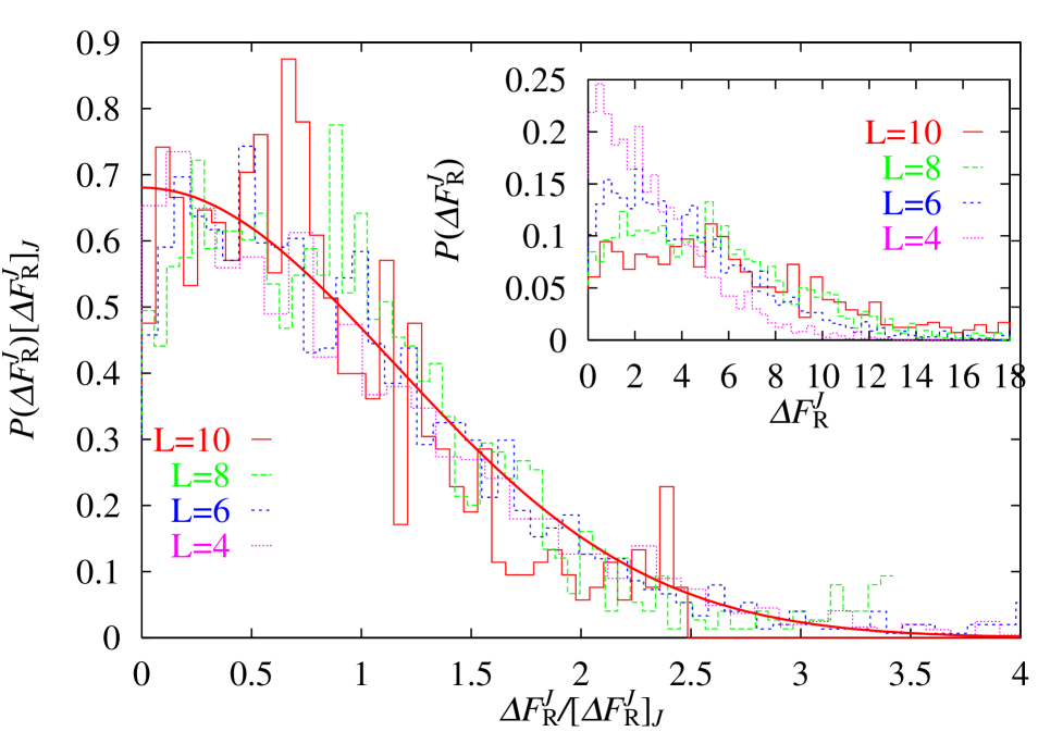
FIG. 8.: Scaling plot of the distribution function of the domain-wall free energy with $T\sim 1.6$. Both axes are scaled by the first moment of the distribution. The solid curve is obtained by fitting the scaling function to a Gaussian formula. The raw data is shown in the inset.

In conclusion, we have proposed a MC method which enable us to estimate the free-energy difference and have successfully applied it to $4d\pm J$ Ising SG model. Our value of $T_{\rm c}$ is in good agreement of the previous results obtained from the numerical simulations and the series expansions. We have presented estimates of two exponents, the stiffness exponent and the fractal dimension. We have also found that low-lying excitations as expected in the droplet theory are realized within one pure state in the SG phase, though we cannot rule out the possibility that there exist many pure states.

A Setting temperature points for the exchange MC method

In this appendix we propose a practical way to determine temperature set which is needed in the exchange MC method. For simplicity, we consider a procedure for setting a temperature point $\beta_{n}$ between two fixed ones, $\beta_{n-1}$ and $\beta_{n+1}$. Our criterion is that acceptance probabilities for the exchange trial with both neighboring temperatures become equal:

$$(\beta_{n-1}-\beta_{n})(E(\beta_{n-1})-E(\beta_{n})) = C,$$ (A1)

$$(\beta_{n}-\beta_{n+1})(E(\beta_{n})-E(\beta_{n+1})) = C,$$ (A2)

where $C$ and $\beta_{n}$ are unknown constants. A formal solution for $\beta_{n}$ is given by

$$\beta_{n}=g(\beta_{n})=\frac{1}{E(\beta_{n-1})-E(\beta_{n+1})}\times(\beta_{n-1}E(\beta_{n-1})$$ (A3)

$$\quad\quad-\beta_{n+1}E(\beta_{n+1})-E(\beta_{n})(\beta_{n-1}-\beta_{n+1})).$$ (A4)

Regarding $\beta^{\prime}=g(\beta)$ as a map of $\beta$ to $\beta^{\prime}$, we find an fixed point of period 2 with $\beta_{n+1}=g(\beta_{n-1})$ and $\beta_{n-1}=g(\beta_{n+1})$. Therefore, we expect a repulsive fixed point between $\beta_{n-1}$ and $\beta_{n+1}$. A new mapping to obtain the fixed point is given by

$$\beta_{n}(t+1)=\frac{1}{2}(\beta_{n}(t)+g(\beta_{n}(t))),$$ (A5)

where $t$ is the iteration step. This iteration scheme can be extended straightforwardly to the case for multiple temperature points. The whole set of temperature is divided into two groups with even-$n$ and odd-$n$. Using the iteration scheme, temperature points of the one group are updated with the other group fixed, alternatively. In actual iterations, the initial temperature points $\{\beta_{n}\}$ are set in a suitable way, for example, equidistant $\beta$. The energy $E(\beta)$ at the initial set of $\beta$ is roughly estimated by short MC simulation and the energy at any temperature between $\beta_{1}$ and $\beta_{M}$ is assumed to be obtained from the MC data, for example, by interpolation technique. The convergence of the iteration is rapidly achieved in many systems we have investigated.

From our experiences so far, efficiency of the EMC method is rather insensitive for the choice of temperature points, when it is applied to systems, such as spin glasses, with non-diverging specific heat at the phase transition. This fact that it is not necessary to specify any parameters before main simulation is, in fact, one of big advantages of the EMC method against the other extended ensemble methods such as the multicanonical MC method and simulated tempering method. Nevertheless we emphasize that a little effort on preparing the temperature points by pre-MC runs following the prescription described above ensures the acceptance ratio almost independent of temperature and so is quite useful.

REFERENCES

- [1] For reviews on spin glasses, K. Binder and A. P. Young, Rev. Mod. Phys. 58, (1986) 801; K. H. Fischer and J. A. Hertz, Spin Glasses Cambridge University Press (1991); A. P. Young, Spin Glasses and Random Fields, World Scientific, Singapore (1997).
- [2] A. T. Ogielski, Phys. Rev. B 32, 7384 (1985).
- [3] R. N. Bhatt and A. P. Young, Phys. Rev. B 37, 5606 (1988).
- [4] N. Kawashima and A. P. Young, Phys. Rev. B 53, R484 (1996).
- [5] E. Marinari, G. Parisi, and J. J. Ruiz-Lorenzo, cond-mat/9802211.
- [6] B. A. Berg and W. Janke, Phys. Rev. Lett. 80, 4771 (1998).
- [7] M. Picco and F. Ritort, cond-mat/9702041.
- [8] E. Marinari, G. Parisi, F. Ricci-Tersenghi and J. J. Ruiz-Lorenzo, J. Phys. A 31, 2611 (1998).
- [9] Y. Ozeki and N. Ito, J. Phys. A 31, 5451 (1998).
- [10] E. Marinari, C. Naitza, F. Zuliani, G. Parisi, M. Picco, and F. Ritort, Phys. Rev. Lett. 81, 1698 (1998).
- [11] W. L. McMillan, Phys. Rev. B 29, 4026 (1984).
- [12] D. S. Fisher and D. Huse, Phys. Rev. B 38, 373 (1998).
- [13] D. S. Fisher and D. Huse, Phys. Rev. B 38, 386 (1998).
- [14] H. Rieger, L. Santen, U. Blasum, M. Diehl, M. Jünger, and G. Rinaldi, J. Phys. A 29, 3939 (1996).
- [15] A. K. Hartmann, cond-mat/9806114.
- [16] J. Maucourt and D. R. Grempel, Phys. Rev. Lett 80, 770 (1998).
- [17] M. Hasenbusch, J. Phys. I France 3, 753 (1993).
- [18] K. Hukushima and K. Nemoto, J. Phys. Soc. Jpn 65, 1604 (1996).
- [19] W. L. McMillan, Phys. Rev. B 30, 476 (1984).
- [20] B. A. Berg and T. Neuhaus, Phys. Lett. B267, 249 (1991).
- [21] E. Marinari and G. Parisi, Europhys. Lett. 19, 451 (1992).
- [22] E. Marinari, G. Parisi and J. J. Ruiz-Lorenzo, Numerical Simulations of Spin Glass Systems, in “Spin Glasses and Random Fields”, edited by A. P. Young (World Scientific, Singapore, 1997), 59.
- [23] A. J. Bray and M. A. Moore, J. Phys. C 17, L463 (1984).
- [24] A. D. Bruce, N. B. Wilding and G. J. Ackland, Phys. Rev. Lett. 79, 3002 (1997).
- [25] Y. Ozeki, J. Phys. Soc. Jpn. 62, 2641 (1993).
- [26] J. C. Curia, G. Parisi and F. Ritort, J. Phys. A26, 6731 (1993).
- [27] D. Badoni, J. C. Ciria, G. Parisi, F. Ritort, J. Pech and J. J. Ruiz-Lorenzo, Europhys. Lett. 21, 495 (1993).
- [28] G. Parisi, F. R. Tersenghi and J. J. Ruiz-Lorenzo, J. Phys. A 29, 7943 (1996).
- [29] R. R. P. Singh and S. Chacravarty, Phys. Rev. Lett., 57, 245 (1986).
- [30] L. Klein, J. Adler, A. Aharony, A. B. Harris and Y. Meir, Phys. Rev. B 43, 11249 (1991).
- [31] F. Matsubara, T. Shirakura and M. Shiomi, Phys. Rev. B 58, R11821 (1998).
- [32] J. M. Kosterlitz and N. Akino, cond-mat/9806339.
- [33] A. J. Bray and M. A. Moore, Phys. Rev. Lett. 58, 57 (1987).
- [34] I. Kondor, J. Phys. A 22, L163 (1989).
- [35] M. Ney-Nifle, Phys. Rev. B 57, 492 (1998).
- [36] V. Azcoiti, E. Follane and F. Ritort, J. Phys. A 28, 3863 (1995).
- [37] M. Nifle and H. J. Hilhorst, Phys. Rev. Lett. 68, 2992 (1992).
- [38] S. Franz, G. Parisi, and M. A. Virasoro, J. Phys. I France 4, 1657 (1994).
- [39] A. J. Bray and M. A. Moore, in Heidelberg Collquium on Glassy Dynamics, Lecture Notes in Physics 275, edited by J. L. van Hemmen and I. Morgenstern (Springer, Berlin, 1986).
- [40] J. D. Reger, R. N. Bhatt and A. P. Young: Phys. Rev. Lett. 64, (1990) 1859.
- [41] M. A. Moore, H. Bokil and B. Drossel, Phys. Rev. Lett. 81, 4252 (1998).