Mesoscopic sensitivity of speckles in disordered nonlinear media
to changes of disordered potential
B.Spivak
Physics Department, University of Washington, Seattle, WA 98195,
USA
A.Zyuzin
A.F.Ioffe Institute, 194021 St.Petersburg, Russia
Abstract
We show that the sensitivity of wave speckle patterns in disordered
nonlinear
media to changes of scattering potential increases with sample size.
For large enough sample size this quantity diverges, which implies
that at given coherent wave incident on a sample there are multiple
solutions for the spatial distribution of
the wave’s density. The number of solutions increases exponentially
with the sample size.
pacs: Suggested PACS index category: 05.20-y, 82.20-w
If a coherent wave described by a field ϕ ( 𝒓 , ϵ ) italic-ϕ 𝒓 italic-ϵ \phi(\mathchoice{{\hbox{\boldmath$\displaystyle r$}}}{{\hbox{\boldmath$\textstyle r$}}}{{\hbox{\boldmath$\scriptstyle r$}}}{{\hbox{\boldmath$\scriptscriptstyle r$}}},\epsilon) n ( 𝒓 , ϵ ) = | ϕ ( 𝒓 , ϵ ) | 2 𝑛 𝒓 italic-ϵ superscript italic-ϕ 𝒓 italic-ϵ 2 n(\mathchoice{{\hbox{\boldmath$\displaystyle r$}}}{{\hbox{\boldmath$\textstyle r$}}}{{\hbox{\boldmath$\scriptstyle r$}}}{{\hbox{\boldmath$\scriptscriptstyle r$}}},\epsilon)=|\phi(\mathchoice{{\hbox{\boldmath$\displaystyle r$}}}{{\hbox{\boldmath$\textstyle r$}}}{{\hbox{\boldmath$\scriptstyle r$}}}{{\hbox{\boldmath$\scriptscriptstyle r$}}},\epsilon)|^{2} n ( 𝒓 , ϵ ) 𝑛 𝒓 italic-ϵ n(\mathchoice{{\hbox{\boldmath$\displaystyle r$}}}{{\hbox{\boldmath$\textstyle r$}}}{{\hbox{\boldmath$\scriptstyle r$}}}{{\hbox{\boldmath$\scriptscriptstyle r$}}},\epsilon) 𝒓 𝒓 \textstyle r ϵ italic-ϵ \epsilon [1-5]
In this article we consider the same question in the case where a wave
propagates in nonlinear media. For the sake of concreteness we consider
the situation where the propagation of the wave is described by a
nonlinear Schrodinger equation
( − 1 2 m ∂ 2 ∂ 𝒓 2 − ϵ + u ( 𝒓 ) + u ~ ( 𝒓 ) ) ϕ ( 𝒓 , ϵ ) = 0 1 2 𝑚 superscript 2 superscript 𝒓 2 italic-ϵ 𝑢 𝒓 ~ 𝑢 𝒓 italic-ϕ 𝒓 italic-ϵ 0 (-\frac{1}{2m}\frac{\partial^{2}}{\partial\mathchoice{{\hbox{\boldmath$\displaystyle r$}}}{{\hbox{\boldmath$\textstyle r$}}}{{\hbox{\boldmath$\scriptstyle r$}}}{{\hbox{\boldmath$\scriptscriptstyle r$}}}^{2}}-\epsilon+u(\mathchoice{{\hbox{\boldmath$\displaystyle r$}}}{{\hbox{\boldmath$\textstyle r$}}}{{\hbox{\boldmath$\scriptstyle r$}}}{{\hbox{\boldmath$\scriptscriptstyle r$}}})+\tilde{u}(\mathchoice{{\hbox{\boldmath$\displaystyle r$}}}{{\hbox{\boldmath$\textstyle r$}}}{{\hbox{\boldmath$\scriptstyle r$}}}{{\hbox{\boldmath$\scriptscriptstyle r$}}}))\phi(\mathchoice{{\hbox{\boldmath$\displaystyle r$}}}{{\hbox{\boldmath$\textstyle r$}}}{{\hbox{\boldmath$\scriptstyle r$}}}{{\hbox{\boldmath$\scriptscriptstyle r$}}},\epsilon)=0 (1)
Here m 𝑚 m u ~ ( 𝒓 ) = β n ( 𝒓 ) ~ 𝑢 𝒓 𝛽 𝑛 𝒓 \tilde{u}(\mathchoice{{\hbox{\boldmath$\displaystyle r$}}}{{\hbox{\boldmath$\textstyle r$}}}{{\hbox{\boldmath$\scriptstyle r$}}}{{\hbox{\boldmath$\scriptscriptstyle r$}}})=\beta n(\mathchoice{{\hbox{\boldmath$\displaystyle r$}}}{{\hbox{\boldmath$\textstyle r$}}}{{\hbox{\boldmath$\scriptstyle r$}}}{{\hbox{\boldmath$\scriptscriptstyle r$}}}) u ( 𝒓 ) 𝑢 𝒓 u(\mathchoice{{\hbox{\boldmath$\displaystyle r$}}}{{\hbox{\boldmath$\textstyle r$}}}{{\hbox{\boldmath$\scriptstyle r$}}}{{\hbox{\boldmath$\scriptscriptstyle r$}}}) [6] [7] [8] u ( 𝒓 ) 𝑢 𝒓 u(\mathchoice{{\hbox{\boldmath$\displaystyle r$}}}{{\hbox{\boldmath$\textstyle r$}}}{{\hbox{\boldmath$\scriptstyle r$}}}{{\hbox{\boldmath$\scriptscriptstyle r$}}}) ⟨ u ( 𝒓 ) ⟩ = 0 delimited-⟨⟩ 𝑢 𝒓 0 \langle u(\mathchoice{{\hbox{\boldmath$\displaystyle r$}}}{{\hbox{\boldmath$\textstyle r$}}}{{\hbox{\boldmath$\scriptstyle r$}}}{{\hbox{\boldmath$\scriptscriptstyle r$}}})\rangle=0 ⟨ u ( 𝒓 ) u ( 𝒓 𝟏 ) ⟩ = π l m 2 δ ( 𝒓 − 𝒓 𝟏 ) delimited-⟨⟩ 𝑢 𝒓 𝑢 subscript 𝒓 1 𝜋 𝑙 superscript 𝑚 2 𝛿 𝒓 subscript 𝒓 1 \langle u(\mathchoice{{\hbox{\boldmath$\displaystyle r$}}}{{\hbox{\boldmath$\textstyle r$}}}{{\hbox{\boldmath$\scriptstyle r$}}}{{\hbox{\boldmath$\scriptscriptstyle r$}}})u(\mathchoice{{\hbox{\boldmath$\displaystyle r_{1}$}}}{{\hbox{\boldmath$\textstyle r_{1}$}}}{{\hbox{\boldmath$\scriptstyle r_{1}$}}}{{\hbox{\boldmath$\scriptscriptstyle r_{1}$}}})\rangle=\frac{\pi}{lm^{2}}\delta(\mathchoice{{\hbox{\boldmath$\displaystyle r$}}}{{\hbox{\boldmath$\textstyle r$}}}{{\hbox{\boldmath$\scriptstyle r$}}}{{\hbox{\boldmath$\scriptscriptstyle r$}}}-\mathchoice{{\hbox{\boldmath$\displaystyle r_{1}$}}}{{\hbox{\boldmath$\textstyle r_{1}$}}}{{\hbox{\boldmath$\scriptstyle r_{1}$}}}{{\hbox{\boldmath$\scriptscriptstyle r_{1}$}}}) ⟨ ⟩
\langle\rangle u ( 𝒓 ) 𝑢 𝒓 u(\mathchoice{{\hbox{\boldmath$\displaystyle r$}}}{{\hbox{\boldmath$\textstyle r$}}}{{\hbox{\boldmath$\scriptstyle r$}}}{{\hbox{\boldmath$\scriptscriptstyle r$}}}) l 𝑙 l l ≫ k − 1 = ( 2 ϵ m ) − 1 2 ) l\gg k^{-1}=(2\epsilon m)^{-\frac{1}{2}}) ϕ 0 ( 𝒓 ) = n 0 exp ( i 𝒌 𝒓 ) subscript italic-ϕ 0 𝒓 subscript 𝑛 0 𝑖 𝒌 𝒓 \phi_{0}(\mathchoice{{\hbox{\boldmath$\displaystyle r$}}}{{\hbox{\boldmath$\textstyle r$}}}{{\hbox{\boldmath$\scriptstyle r$}}}{{\hbox{\boldmath$\scriptscriptstyle r$}}})=\sqrt{n_{0}}\exp(i\mathchoice{{\hbox{\boldmath$\displaystyle k$}}}{{\hbox{\boldmath$\textstyle k$}}}{{\hbox{\boldmath$\scriptstyle k$}}}{{\hbox{\boldmath$\scriptscriptstyle k$}}}\mathchoice{{\hbox{\boldmath$\displaystyle r$}}}{{\hbox{\boldmath$\textstyle r$}}}{{\hbox{\boldmath$\scriptstyle r$}}}{{\hbox{\boldmath$\scriptscriptstyle r$}}}) 𝒌 𝒌 \textstyle k L ≫ l much-greater-than 𝐿 𝑙 L\gg l n ( 𝒓 ) 𝑛 𝒓 n(\mathchoice{{\hbox{\boldmath$\displaystyle r$}}}{{\hbox{\boldmath$\textstyle r$}}}{{\hbox{\boldmath$\scriptstyle r$}}}{{\hbox{\boldmath$\scriptscriptstyle r$}}}) u ( 𝒓 ) 𝑢 𝒓 u(\mathchoice{{\hbox{\boldmath$\displaystyle r$}}}{{\hbox{\boldmath$\textstyle r$}}}{{\hbox{\boldmath$\scriptstyle r$}}}{{\hbox{\boldmath$\scriptscriptstyle r$}}}) L 𝐿 L n 0 subscript 𝑛 0 n_{0} β 𝛽 \beta L 𝐿 L β 𝛽 \beta [6]
The 𝒓 𝒓 \textstyle r ⟨ n ( 𝒓 , ϵ ) ⟩ delimited-⟨⟩ 𝑛 𝒓 italic-ϵ \langle n(\mathchoice{{\hbox{\boldmath$\displaystyle r$}}}{{\hbox{\boldmath$\textstyle r$}}}{{\hbox{\boldmath$\scriptstyle r$}}}{{\hbox{\boldmath$\scriptscriptstyle r$}}},\epsilon)\rangle [9] | β n 0 | ≪ ϵ k l m much-less-than 𝛽 subscript 𝑛 0 italic-ϵ 𝑘 𝑙 𝑚 |\beta n_{0}|\ll\sqrt{\frac{\epsilon k}{lm}} D = l k 3 m 𝐷 𝑙 𝑘 3 𝑚 D=\frac{lk}{3m} β n ( 𝒓 ) 𝛽 𝑛 𝒓 \beta n(\mathchoice{{\hbox{\boldmath$\displaystyle r$}}}{{\hbox{\boldmath$\textstyle r$}}}{{\hbox{\boldmath$\scriptstyle r$}}}{{\hbox{\boldmath$\scriptscriptstyle r$}}}) [11,4] [10] ⟨ n ( 𝒓 ) ⟩ = n 0 delimited-⟨⟩ 𝑛 𝒓 subscript 𝑛 0 \langle n(\mathchoice{{\hbox{\boldmath$\displaystyle r$}}}{{\hbox{\boldmath$\textstyle r$}}}{{\hbox{\boldmath$\scriptstyle r$}}}{{\hbox{\boldmath$\scriptscriptstyle r$}}})\rangle=n_{0}
We can characterize the speckle pattern n ( 𝒓 ) 𝑛 𝒓 n(\mathchoice{{\hbox{\boldmath$\displaystyle r$}}}{{\hbox{\boldmath$\textstyle r$}}}{{\hbox{\boldmath$\scriptstyle r$}}}{{\hbox{\boldmath$\scriptscriptstyle r$}}}) Δ u ( 𝒓 ) = u ′ ( 𝒓 ) − u ( 𝒓 ) Δ 𝑢 𝒓 superscript 𝑢 ′ 𝒓 𝑢 𝒓 \Delta u(\mathchoice{{\hbox{\boldmath$\displaystyle r$}}}{{\hbox{\boldmath$\textstyle r$}}}{{\hbox{\boldmath$\scriptstyle r$}}}{{\hbox{\boldmath$\scriptscriptstyle r$}}})=u^{\prime}(\mathchoice{{\hbox{\boldmath$\displaystyle r$}}}{{\hbox{\boldmath$\textstyle r$}}}{{\hbox{\boldmath$\scriptstyle r$}}}{{\hbox{\boldmath$\scriptscriptstyle r$}}})-u(\mathchoice{{\hbox{\boldmath$\displaystyle r$}}}{{\hbox{\boldmath$\textstyle r$}}}{{\hbox{\boldmath$\scriptstyle r$}}}{{\hbox{\boldmath$\scriptscriptstyle r$}}}) ⟨ δ n ( 𝒓 ) δ n ( 𝒓 1 ) ⟩ delimited-⟨⟩ 𝛿 𝑛 𝒓 𝛿 𝑛 subscript 𝒓 1 \langle\delta n(\mathchoice{{\hbox{\boldmath$\displaystyle r$}}}{{\hbox{\boldmath$\textstyle r$}}}{{\hbox{\boldmath$\scriptstyle r$}}}{{\hbox{\boldmath$\scriptscriptstyle r$}}})\delta n(\mathchoice{{\hbox{\boldmath$\displaystyle r$}}}{{\hbox{\boldmath$\textstyle r$}}}{{\hbox{\boldmath$\scriptstyle r$}}}{{\hbox{\boldmath$\scriptscriptstyle r$}}}_{1})\rangle K ( 𝒓 , 𝒓 1 ) = ⟨ ⟨ Δ n ( 𝒓 ) Δ n ( 𝒓 𝟏 ) ⟩ ⟩ 𝐾 𝒓 subscript 𝒓 1 delimited-⟨⟩ delimited-⟨⟩ Δ 𝑛 𝒓 Δ 𝑛 subscript 𝒓 1 K(\mathchoice{{\hbox{\boldmath$\displaystyle r$}}}{{\hbox{\boldmath$\textstyle r$}}}{{\hbox{\boldmath$\scriptstyle r$}}}{{\hbox{\boldmath$\scriptscriptstyle r$}}},\mathchoice{{\hbox{\boldmath$\displaystyle r$}}}{{\hbox{\boldmath$\textstyle r$}}}{{\hbox{\boldmath$\scriptstyle r$}}}{{\hbox{\boldmath$\scriptscriptstyle r$}}}_{1})=\langle\langle\Delta n(\mathchoice{{\hbox{\boldmath$\displaystyle r$}}}{{\hbox{\boldmath$\textstyle r$}}}{{\hbox{\boldmath$\scriptstyle r$}}}{{\hbox{\boldmath$\scriptscriptstyle r$}}})\Delta n(\mathchoice{{\hbox{\boldmath$\displaystyle r_{1}$}}}{{\hbox{\boldmath$\textstyle r_{1}$}}}{{\hbox{\boldmath$\scriptstyle r_{1}$}}}{{\hbox{\boldmath$\scriptscriptstyle r_{1}$}}})\rangle\rangle δ n ( 𝒓 ) = n ( 𝒓 ) − ⟨ n ( 𝒓 ) ⟩ 𝛿 𝑛 𝒓 𝑛 𝒓 delimited-⟨⟩ 𝑛 𝒓 \delta n(\mathchoice{{\hbox{\boldmath$\displaystyle r$}}}{{\hbox{\boldmath$\textstyle r$}}}{{\hbox{\boldmath$\scriptstyle r$}}}{{\hbox{\boldmath$\scriptscriptstyle r$}}})=n(\mathchoice{{\hbox{\boldmath$\displaystyle r$}}}{{\hbox{\boldmath$\textstyle r$}}}{{\hbox{\boldmath$\scriptstyle r$}}}{{\hbox{\boldmath$\scriptscriptstyle r$}}})-\langle n(\mathchoice{{\hbox{\boldmath$\displaystyle r$}}}{{\hbox{\boldmath$\textstyle r$}}}{{\hbox{\boldmath$\scriptstyle r$}}}{{\hbox{\boldmath$\scriptscriptstyle r$}}})\rangle Δ n ( 𝒓 ) = n ′ ( 𝒓 , { u ′ ( 𝒓 ) } ) − n ( 𝒓 , { u ( 𝒓 ) } ) Δ 𝑛 𝒓 superscript 𝑛 ′ 𝒓 superscript 𝑢 ′ 𝒓 𝑛 𝒓 𝑢 𝒓 \Delta n(\mathchoice{{\hbox{\boldmath$\displaystyle r$}}}{{\hbox{\boldmath$\textstyle r$}}}{{\hbox{\boldmath$\scriptstyle r$}}}{{\hbox{\boldmath$\scriptscriptstyle r$}}})=n^{\prime}(\mathchoice{{\hbox{\boldmath$\displaystyle r$}}}{{\hbox{\boldmath$\textstyle r$}}}{{\hbox{\boldmath$\scriptstyle r$}}}{{\hbox{\boldmath$\scriptscriptstyle r$}}},\{u^{\prime}(\mathchoice{{\hbox{\boldmath$\displaystyle r$}}}{{\hbox{\boldmath$\textstyle r$}}}{{\hbox{\boldmath$\scriptstyle r$}}}{{\hbox{\boldmath$\scriptscriptstyle r$}}})\})-n(\mathchoice{{\hbox{\boldmath$\displaystyle r$}}}{{\hbox{\boldmath$\textstyle r$}}}{{\hbox{\boldmath$\scriptstyle r$}}}{{\hbox{\boldmath$\scriptscriptstyle r$}}},\{u(\mathchoice{{\hbox{\boldmath$\displaystyle r$}}}{{\hbox{\boldmath$\textstyle r$}}}{{\hbox{\boldmath$\scriptstyle r$}}}{{\hbox{\boldmath$\scriptscriptstyle r$}}})\}) n ( ϵ , 𝒓 , { u ( 𝒓 ) } ) 𝑛 italic-ϵ 𝒓 𝑢 𝒓 n(\epsilon,\mathchoice{{\hbox{\boldmath$\displaystyle r$}}}{{\hbox{\boldmath$\textstyle r$}}}{{\hbox{\boldmath$\scriptstyle r$}}}{{\hbox{\boldmath$\scriptscriptstyle r$}}},\{u(\mathchoice{{\hbox{\boldmath$\displaystyle r$}}}{{\hbox{\boldmath$\textstyle r$}}}{{\hbox{\boldmath$\scriptstyle r$}}}{{\hbox{\boldmath$\scriptscriptstyle r$}}})\}) n ′ ( ϵ , 𝒓 , { u ′ ( 𝒓 ) } ) superscript 𝑛 ′ italic-ϵ 𝒓 superscript 𝑢 ′ 𝒓 n^{\prime}(\epsilon,\mathchoice{{\hbox{\boldmath$\displaystyle r$}}}{{\hbox{\boldmath$\textstyle r$}}}{{\hbox{\boldmath$\scriptstyle r$}}}{{\hbox{\boldmath$\scriptscriptstyle r$}}},\{u^{\prime}(\mathchoice{{\hbox{\boldmath$\displaystyle r$}}}{{\hbox{\boldmath$\textstyle r$}}}{{\hbox{\boldmath$\scriptstyle r$}}}{{\hbox{\boldmath$\scriptscriptstyle r$}}})\}) u ( 𝒓 ) 𝑢 𝒓 u(\mathchoice{{\hbox{\boldmath$\displaystyle r$}}}{{\hbox{\boldmath$\textstyle r$}}}{{\hbox{\boldmath$\scriptstyle r$}}}{{\hbox{\boldmath$\scriptscriptstyle r$}}}) u ′ ( 𝒓 ) superscript 𝑢 ′ 𝒓 u^{\prime}(\mathchoice{{\hbox{\boldmath$\displaystyle r$}}}{{\hbox{\boldmath$\textstyle r$}}}{{\hbox{\boldmath$\scriptstyle r$}}}{{\hbox{\boldmath$\scriptscriptstyle r$}}}) ⟨ ⟨ ⟩ ⟩ delimited-⟨⟩
\langle\langle\rangle\rangle u ( 𝒓 ) 𝑢 𝒓 u(\mathchoice{{\hbox{\boldmath$\displaystyle r$}}}{{\hbox{\boldmath$\textstyle r$}}}{{\hbox{\boldmath$\scriptstyle r$}}}{{\hbox{\boldmath$\scriptscriptstyle r$}}}) Δ u ( 𝒓 ) Δ 𝑢 𝒓 \Delta u(\mathchoice{{\hbox{\boldmath$\displaystyle r$}}}{{\hbox{\boldmath$\textstyle r$}}}{{\hbox{\boldmath$\scriptstyle r$}}}{{\hbox{\boldmath$\scriptscriptstyle r$}}}) ⟨ ⟨ u ( 𝒓 ) u ′ ( 𝒓 𝟏 ) ⟩ ⟩ = U 2 exp ( | 𝒓 − 𝒓 1 | r 0 ) delimited-⟨⟩ delimited-⟨⟩ 𝑢 𝒓 superscript 𝑢 ′ subscript 𝒓 1 superscript 𝑈 2 𝒓 subscript 𝒓 1 subscript 𝑟 0 \langle\langle u(\mathchoice{{\hbox{\boldmath$\displaystyle r$}}}{{\hbox{\boldmath$\textstyle r$}}}{{\hbox{\boldmath$\scriptstyle r$}}}{{\hbox{\boldmath$\scriptscriptstyle r$}}})u^{\prime}(\mathchoice{{\hbox{\boldmath$\displaystyle r_{1}$}}}{{\hbox{\boldmath$\textstyle r_{1}$}}}{{\hbox{\boldmath$\scriptstyle r_{1}$}}}{{\hbox{\boldmath$\scriptscriptstyle r_{1}$}}})\rangle\rangle=U^{2}\exp(\frac{|\mathchoice{{\hbox{\boldmath$\displaystyle r$}}}{{\hbox{\boldmath$\textstyle r$}}}{{\hbox{\boldmath$\scriptstyle r$}}}{{\hbox{\boldmath$\scriptscriptstyle r$}}}-\mathchoice{{\hbox{\boldmath$\displaystyle r$}}}{{\hbox{\boldmath$\textstyle r$}}}{{\hbox{\boldmath$\scriptstyle r$}}}{{\hbox{\boldmath$\scriptscriptstyle r$}}}_{1}|}{r_{0}}) K ( 𝒓 , 𝒓 1 ) 𝐾 𝒓 subscript 𝒓 1 K(\mathchoice{{\hbox{\boldmath$\displaystyle r$}}}{{\hbox{\boldmath$\textstyle r$}}}{{\hbox{\boldmath$\scriptstyle r$}}}{{\hbox{\boldmath$\scriptscriptstyle r$}}},\mathchoice{{\hbox{\boldmath$\displaystyle r$}}}{{\hbox{\boldmath$\textstyle r$}}}{{\hbox{\boldmath$\scriptstyle r$}}}{{\hbox{\boldmath$\scriptscriptstyle r$}}}_{1}) | 𝒓 − 𝒓 1 | ≫ l much-greater-than 𝒓 subscript 𝒓 1 𝑙 |\mathchoice{{\hbox{\boldmath$\displaystyle r$}}}{{\hbox{\boldmath$\textstyle r$}}}{{\hbox{\boldmath$\scriptstyle r$}}}{{\hbox{\boldmath$\scriptscriptstyle r$}}}-\mathchoice{{\hbox{\boldmath$\displaystyle r$}}}{{\hbox{\boldmath$\textstyle r$}}}{{\hbox{\boldmath$\scriptstyle r$}}}{{\hbox{\boldmath$\scriptscriptstyle r$}}}_{1}|\gg l Δ u ( 𝒓 ) Δ 𝑢 𝒓 \Delta u(\mathchoice{{\hbox{\boldmath$\displaystyle r$}}}{{\hbox{\boldmath$\textstyle r$}}}{{\hbox{\boldmath$\scriptstyle r$}}}{{\hbox{\boldmath$\scriptscriptstyle r$}}}) [4,11]
d d 𝒓 δ 𝑱 ( 𝒓 ) = 0 ; δ 𝑱 ( 𝒓 ) = − D d d 𝒓 δ n ( 𝒓 ) + 𝑱 e x t ( 𝒓 ) ; formulae-sequence 𝑑 𝑑 𝒓 𝛿 𝑱 𝒓 0 𝛿 𝑱 𝒓 𝐷 𝑑 𝑑 𝒓 𝛿 𝑛 𝒓 subscript 𝑱 𝑒 𝑥 𝑡 𝒓 \frac{d}{d\mathchoice{{\hbox{\boldmath$\displaystyle r$}}}{{\hbox{\boldmath$\textstyle r$}}}{{\hbox{\boldmath$\scriptstyle r$}}}{{\hbox{\boldmath$\scriptscriptstyle r$}}}}\delta\mathchoice{{\hbox{\boldmath$\displaystyle J$}}}{{\hbox{\boldmath$\textstyle J$}}}{{\hbox{\boldmath$\scriptstyle J$}}}{{\hbox{\boldmath$\scriptscriptstyle J$}}}(\mathchoice{{\hbox{\boldmath$\displaystyle r$}}}{{\hbox{\boldmath$\textstyle r$}}}{{\hbox{\boldmath$\scriptstyle r$}}}{{\hbox{\boldmath$\scriptscriptstyle r$}}})=0;\quad\delta\mathchoice{{\hbox{\boldmath$\displaystyle J$}}}{{\hbox{\boldmath$\textstyle J$}}}{{\hbox{\boldmath$\scriptstyle J$}}}{{\hbox{\boldmath$\scriptscriptstyle J$}}}(\mathchoice{{\hbox{\boldmath$\displaystyle r$}}}{{\hbox{\boldmath$\textstyle r$}}}{{\hbox{\boldmath$\scriptstyle r$}}}{{\hbox{\boldmath$\scriptscriptstyle r$}}})=-D\frac{d}{d\mathchoice{{\hbox{\boldmath$\displaystyle r$}}}{{\hbox{\boldmath$\textstyle r$}}}{{\hbox{\boldmath$\scriptstyle r$}}}{{\hbox{\boldmath$\scriptscriptstyle r$}}}}\delta n(\mathchoice{{\hbox{\boldmath$\displaystyle r$}}}{{\hbox{\boldmath$\textstyle r$}}}{{\hbox{\boldmath$\scriptstyle r$}}}{{\hbox{\boldmath$\scriptscriptstyle r$}}})+\mathchoice{{\hbox{\boldmath$\displaystyle J$}}}{{\hbox{\boldmath$\textstyle J$}}}{{\hbox{\boldmath$\scriptstyle J$}}}{{\hbox{\boldmath$\scriptscriptstyle J$}}}_{ext}(\mathchoice{{\hbox{\boldmath$\displaystyle r$}}}{{\hbox{\boldmath$\textstyle r$}}}{{\hbox{\boldmath$\scriptstyle r$}}}{{\hbox{\boldmath$\scriptscriptstyle r$}}}); (2)
𝑱 e x t ( 𝒓 , { u ′ ( 𝒓 ) } ) = 𝑱 e x t ( 𝒓 , { u ( 𝒓 ) } ) + ∫ 𝑑 𝒓 ′ δ 𝑱 e x t ( 𝒓 ) δ u ( 𝒓 ′ ) ( Δ u ( 𝒓 ′ ) + Δ u ~ ( 𝒓 ′ ) ) subscript 𝑱 𝑒 𝑥 𝑡 𝒓 superscript 𝑢 ′ 𝒓 subscript 𝑱 𝑒 𝑥 𝑡 𝒓 𝑢 𝒓 differential-d superscript 𝒓 ′ 𝛿 subscript 𝑱 𝑒 𝑥 𝑡 𝒓 𝛿 𝑢 superscript 𝒓 ′ Δ 𝑢 superscript 𝒓 ′ Δ ~ 𝑢 superscript 𝒓 ′ \mathchoice{{\hbox{\boldmath$\displaystyle J$}}}{{\hbox{\boldmath$\textstyle J$}}}{{\hbox{\boldmath$\scriptstyle J$}}}{{\hbox{\boldmath$\scriptscriptstyle J$}}}_{ext}(\mathchoice{{\hbox{\boldmath$\displaystyle r$}}}{{\hbox{\boldmath$\textstyle r$}}}{{\hbox{\boldmath$\scriptstyle r$}}}{{\hbox{\boldmath$\scriptscriptstyle r$}}},\{u^{\prime}(\mathchoice{{\hbox{\boldmath$\displaystyle r$}}}{{\hbox{\boldmath$\textstyle r$}}}{{\hbox{\boldmath$\scriptstyle r$}}}{{\hbox{\boldmath$\scriptscriptstyle r$}}})\})=\mathchoice{{\hbox{\boldmath$\displaystyle J$}}}{{\hbox{\boldmath$\textstyle J$}}}{{\hbox{\boldmath$\scriptstyle J$}}}{{\hbox{\boldmath$\scriptscriptstyle J$}}}_{ext}(\mathchoice{{\hbox{\boldmath$\displaystyle r$}}}{{\hbox{\boldmath$\textstyle r$}}}{{\hbox{\boldmath$\scriptstyle r$}}}{{\hbox{\boldmath$\scriptscriptstyle r$}}},\{u(\mathchoice{{\hbox{\boldmath$\displaystyle r$}}}{{\hbox{\boldmath$\textstyle r$}}}{{\hbox{\boldmath$\scriptstyle r$}}}{{\hbox{\boldmath$\scriptscriptstyle r$}}})\})+\int d\mathchoice{{\hbox{\boldmath$\displaystyle r$}}}{{\hbox{\boldmath$\textstyle r$}}}{{\hbox{\boldmath$\scriptstyle r$}}}{{\hbox{\boldmath$\scriptscriptstyle r$}}}^{\prime}\frac{\delta\mathchoice{{\hbox{\boldmath$\displaystyle J$}}}{{\hbox{\boldmath$\textstyle J$}}}{{\hbox{\boldmath$\scriptstyle J$}}}{{\hbox{\boldmath$\scriptscriptstyle J$}}}_{ext}(\mathchoice{{\hbox{\boldmath$\displaystyle r$}}}{{\hbox{\boldmath$\textstyle r$}}}{{\hbox{\boldmath$\scriptstyle r$}}}{{\hbox{\boldmath$\scriptscriptstyle r$}}})}{\delta u(\mathchoice{{\hbox{\boldmath$\displaystyle r$}}}{{\hbox{\boldmath$\textstyle r$}}}{{\hbox{\boldmath$\scriptstyle r$}}}{{\hbox{\boldmath$\scriptscriptstyle r$}}}^{\prime})}(\Delta u(\mathchoice{{\hbox{\boldmath$\displaystyle r$}}}{{\hbox{\boldmath$\textstyle r$}}}{{\hbox{\boldmath$\scriptstyle r$}}}{{\hbox{\boldmath$\scriptscriptstyle r$}}}^{\prime})+\Delta\tilde{u}(\mathchoice{{\hbox{\boldmath$\displaystyle r$}}}{{\hbox{\boldmath$\textstyle r$}}}{{\hbox{\boldmath$\scriptstyle r$}}}{{\hbox{\boldmath$\scriptscriptstyle r$}}}^{\prime})) (3)
⟨ J e x t i ( 𝒓 ) J e x t j ( 𝒓 1 ) ⟩ = 2 π l 3 m 2 ⟨ n ( 𝒓 ) ⟩ 2 δ ( 𝒓 − 𝒓 𝟏 ) δ i j delimited-⟨⟩ subscript superscript 𝐽 𝑖 𝑒 𝑥 𝑡 𝒓 subscript superscript 𝐽 𝑗 𝑒 𝑥 𝑡 subscript 𝒓 1 2 𝜋 𝑙 3 superscript 𝑚 2 superscript delimited-⟨⟩ 𝑛 𝒓 2 𝛿 𝒓 subscript 𝒓 1 subscript 𝛿 𝑖 𝑗 \langle J^{i}_{ext}(\mathchoice{{\hbox{\boldmath$\displaystyle r$}}}{{\hbox{\boldmath$\textstyle r$}}}{{\hbox{\boldmath$\scriptstyle r$}}}{{\hbox{\boldmath$\scriptscriptstyle r$}}})J^{j}_{ext}(\mathchoice{{\hbox{\boldmath$\displaystyle r$}}}{{\hbox{\boldmath$\textstyle r$}}}{{\hbox{\boldmath$\scriptstyle r$}}}{{\hbox{\boldmath$\scriptscriptstyle r$}}}_{1})\rangle=\frac{2\pi l}{3m^{2}}\langle n(\mathchoice{{\hbox{\boldmath$\displaystyle r$}}}{{\hbox{\boldmath$\textstyle r$}}}{{\hbox{\boldmath$\scriptstyle r$}}}{{\hbox{\boldmath$\scriptscriptstyle r$}}})\rangle^{2}\delta(\mathchoice{{\hbox{\boldmath$\displaystyle r$}}}{{\hbox{\boldmath$\textstyle r$}}}{{\hbox{\boldmath$\scriptstyle r$}}}{{\hbox{\boldmath$\scriptscriptstyle r$}}}-\mathchoice{{\hbox{\boldmath$\displaystyle r_{1}$}}}{{\hbox{\boldmath$\textstyle r_{1}$}}}{{\hbox{\boldmath$\scriptstyle r_{1}$}}}{{\hbox{\boldmath$\scriptscriptstyle r_{1}$}}})\delta_{ij} (4)
⟨ δ J e x t i ( 𝒓 ) δ u ( 𝒓 ′ ) δ J e x t j ( 𝒓 1 ) δ u ( 𝒓 1 ′ ) ⟩ = 6 π l k 2 δ i j δ ( 𝒓 − 𝒓 1 ) { G ( 𝒓 ′ , 𝒓 1 ′ ) ⟨ n ( 𝒓 ) ⟩ × \displaystyle\langle\frac{\delta J^{i}_{ext}(\mathchoice{{\hbox{\boldmath$\displaystyle r$}}}{{\hbox{\boldmath$\textstyle r$}}}{{\hbox{\boldmath$\scriptstyle r$}}}{{\hbox{\boldmath$\scriptscriptstyle r$}}})}{\delta u(\mathchoice{{\hbox{\boldmath$\displaystyle r$}}}{{\hbox{\boldmath$\textstyle r$}}}{{\hbox{\boldmath$\scriptstyle r$}}}{{\hbox{\boldmath$\scriptscriptstyle r$}}}^{\prime})}\frac{\delta J^{j}_{ext}(\mathchoice{{\hbox{\boldmath$\displaystyle r$}}}{{\hbox{\boldmath$\textstyle r$}}}{{\hbox{\boldmath$\scriptstyle r$}}}{{\hbox{\boldmath$\scriptscriptstyle r$}}}_{1})}{\delta u(\mathchoice{{\hbox{\boldmath$\displaystyle r$}}}{{\hbox{\boldmath$\textstyle r$}}}{{\hbox{\boldmath$\scriptstyle r$}}}{{\hbox{\boldmath$\scriptscriptstyle r$}}}^{\prime}_{1})}\rangle=\frac{6\pi}{lk^{2}}\delta_{ij}\delta(\mathchoice{{\hbox{\boldmath$\displaystyle r$}}}{{\hbox{\boldmath$\textstyle r$}}}{{\hbox{\boldmath$\scriptstyle r$}}}{{\hbox{\boldmath$\scriptscriptstyle r$}}}-\mathchoice{{\hbox{\boldmath$\displaystyle r$}}}{{\hbox{\boldmath$\textstyle r$}}}{{\hbox{\boldmath$\scriptstyle r$}}}{{\hbox{\boldmath$\scriptscriptstyle r$}}}_{1})\{G(\mathchoice{{\hbox{\boldmath$\displaystyle r$}}}{{\hbox{\boldmath$\textstyle r$}}}{{\hbox{\boldmath$\scriptstyle r$}}}{{\hbox{\boldmath$\scriptscriptstyle r$}}}^{\prime},\mathchoice{{\hbox{\boldmath$\displaystyle r$}}}{{\hbox{\boldmath$\textstyle r$}}}{{\hbox{\boldmath$\scriptstyle r$}}}{{\hbox{\boldmath$\scriptscriptstyle r$}}}^{\prime}_{1})\langle n(\mathchoice{{\hbox{\boldmath$\displaystyle r$}}}{{\hbox{\boldmath$\textstyle r$}}}{{\hbox{\boldmath$\scriptstyle r$}}}{{\hbox{\boldmath$\scriptscriptstyle r$}}})\rangle\times (5)
( ⟨ n ( 𝒓 1 ′ ) ⟩ G ( 𝒓 ′ , 𝒓 ) + ⟨ n ( 𝒓 ′ ) ⟩ G ( 𝒓 1 ′ , 𝒓 ) ) − ⟨ n ( 𝒓 ′ ) ⟩ ⟨ n ( 𝒓 1 ′ ) ⟩ G ( 𝒓 ′ , 𝒓 ) ) G ( 𝒓 1 ′ , 𝒓 ) } \displaystyle(\langle n(\mathchoice{{\hbox{\boldmath$\displaystyle r$}}}{{\hbox{\boldmath$\textstyle r$}}}{{\hbox{\boldmath$\scriptstyle r$}}}{{\hbox{\boldmath$\scriptscriptstyle r$}}}^{\prime}_{1})\rangle G(\mathchoice{{\hbox{\boldmath$\displaystyle r$}}}{{\hbox{\boldmath$\textstyle r$}}}{{\hbox{\boldmath$\scriptstyle r$}}}{{\hbox{\boldmath$\scriptscriptstyle r$}}}^{\prime},\mathchoice{{\hbox{\boldmath$\displaystyle r$}}}{{\hbox{\boldmath$\textstyle r$}}}{{\hbox{\boldmath$\scriptstyle r$}}}{{\hbox{\boldmath$\scriptscriptstyle r$}}})+\langle n(\mathchoice{{\hbox{\boldmath$\displaystyle r$}}}{{\hbox{\boldmath$\textstyle r$}}}{{\hbox{\boldmath$\scriptstyle r$}}}{{\hbox{\boldmath$\scriptscriptstyle r$}}}^{\prime})\rangle G(\mathchoice{{\hbox{\boldmath$\displaystyle r$}}}{{\hbox{\boldmath$\textstyle r$}}}{{\hbox{\boldmath$\scriptstyle r$}}}{{\hbox{\boldmath$\scriptscriptstyle r$}}}^{\prime}_{1},\mathchoice{{\hbox{\boldmath$\displaystyle r$}}}{{\hbox{\boldmath$\textstyle r$}}}{{\hbox{\boldmath$\scriptstyle r$}}}{{\hbox{\boldmath$\scriptscriptstyle r$}}}))-\langle n(\mathchoice{{\hbox{\boldmath$\displaystyle r$}}}{{\hbox{\boldmath$\textstyle r$}}}{{\hbox{\boldmath$\scriptstyle r$}}}{{\hbox{\boldmath$\scriptscriptstyle r$}}}^{\prime})\rangle\langle n(\mathchoice{{\hbox{\boldmath$\displaystyle r$}}}{{\hbox{\boldmath$\textstyle r$}}}{{\hbox{\boldmath$\scriptstyle r$}}}{{\hbox{\boldmath$\scriptscriptstyle r$}}}^{\prime}_{1})\rangle G(\mathchoice{{\hbox{\boldmath$\displaystyle r$}}}{{\hbox{\boldmath$\textstyle r$}}}{{\hbox{\boldmath$\scriptstyle r$}}}{{\hbox{\boldmath$\scriptscriptstyle r$}}}^{\prime},\mathchoice{{\hbox{\boldmath$\displaystyle r$}}}{{\hbox{\boldmath$\textstyle r$}}}{{\hbox{\boldmath$\scriptstyle r$}}}{{\hbox{\boldmath$\scriptscriptstyle r$}}}))G(\mathchoice{{\hbox{\boldmath$\displaystyle r$}}}{{\hbox{\boldmath$\textstyle r$}}}{{\hbox{\boldmath$\scriptstyle r$}}}{{\hbox{\boldmath$\scriptscriptstyle r$}}}^{\prime}_{1},\mathchoice{{\hbox{\boldmath$\displaystyle r$}}}{{\hbox{\boldmath$\textstyle r$}}}{{\hbox{\boldmath$\scriptstyle r$}}}{{\hbox{\boldmath$\scriptscriptstyle r$}}})\} (6)
Δ u ~ ( 𝒓 ) = u ′ ~ ( 𝒓 ) − u ~ ( 𝒓 ) = β Δ n ( 𝒓 ) Δ ~ 𝑢 𝒓 ~ superscript 𝑢 ′ 𝒓 ~ 𝑢 𝒓 𝛽 Δ 𝑛 𝒓 \Delta\tilde{u}(\mathchoice{{\hbox{\boldmath$\displaystyle r$}}}{{\hbox{\boldmath$\textstyle r$}}}{{\hbox{\boldmath$\scriptstyle r$}}}{{\hbox{\boldmath$\scriptscriptstyle r$}}})=\tilde{u^{\prime}}(\mathchoice{{\hbox{\boldmath$\displaystyle r$}}}{{\hbox{\boldmath$\textstyle r$}}}{{\hbox{\boldmath$\scriptstyle r$}}}{{\hbox{\boldmath$\scriptscriptstyle r$}}})-\tilde{u}(\mathchoice{{\hbox{\boldmath$\displaystyle r$}}}{{\hbox{\boldmath$\textstyle r$}}}{{\hbox{\boldmath$\scriptstyle r$}}}{{\hbox{\boldmath$\scriptscriptstyle r$}}})=\beta\Delta n(\mathchoice{{\hbox{\boldmath$\displaystyle r$}}}{{\hbox{\boldmath$\textstyle r$}}}{{\hbox{\boldmath$\scriptstyle r$}}}{{\hbox{\boldmath$\scriptscriptstyle r$}}}) (7)
where G ( 𝒓 , 𝒓 𝟏 ) 𝐺 𝒓 subscript 𝒓 1 G(\mathchoice{{\hbox{\boldmath$\displaystyle r$}}}{{\hbox{\boldmath$\textstyle r$}}}{{\hbox{\boldmath$\scriptstyle r$}}}{{\hbox{\boldmath$\scriptscriptstyle r$}}},\mathchoice{{\hbox{\boldmath$\displaystyle r_{1}$}}}{{\hbox{\boldmath$\textstyle r_{1}$}}}{{\hbox{\boldmath$\scriptstyle r_{1}$}}}{{\hbox{\boldmath$\scriptscriptstyle r_{1}$}}})
− d 2 d 2 𝒓 G ( 𝒓 , 𝒓 1 ) = δ ( 𝒓 − 𝒓 1 ) ; superscript 𝑑 2 superscript 𝑑 2 𝒓 𝐺 𝒓 subscript 𝒓 1 𝛿 𝒓 subscript 𝒓 1 -\frac{d^{2}}{d^{2}\mathchoice{{\hbox{\boldmath$\displaystyle r$}}}{{\hbox{\boldmath$\textstyle r$}}}{{\hbox{\boldmath$\scriptstyle r$}}}{{\hbox{\boldmath$\scriptscriptstyle r$}}}}G(\mathchoice{{\hbox{\boldmath$\displaystyle r$}}}{{\hbox{\boldmath$\textstyle r$}}}{{\hbox{\boldmath$\scriptstyle r$}}}{{\hbox{\boldmath$\scriptscriptstyle r$}}},\mathchoice{{\hbox{\boldmath$\displaystyle r$}}}{{\hbox{\boldmath$\textstyle r$}}}{{\hbox{\boldmath$\scriptstyle r$}}}{{\hbox{\boldmath$\scriptscriptstyle r$}}}_{1})=\delta(\mathchoice{{\hbox{\boldmath$\displaystyle r$}}}{{\hbox{\boldmath$\textstyle r$}}}{{\hbox{\boldmath$\scriptstyle r$}}}{{\hbox{\boldmath$\scriptscriptstyle r$}}}-\mathchoice{{\hbox{\boldmath$\displaystyle r$}}}{{\hbox{\boldmath$\textstyle r$}}}{{\hbox{\boldmath$\scriptstyle r$}}}{{\hbox{\boldmath$\scriptscriptstyle r$}}}_{1}); (8)
𝑱 ( 𝒓 ) = 1 2 m I m ϕ ∗ ( 𝒓 ) d d 𝒓 ϕ ( 𝒓 ) 𝑱 𝒓 1 2 𝑚 𝐼 𝑚 superscript italic-ϕ 𝒓 𝑑 𝑑 𝒓 italic-ϕ 𝒓 \mathchoice{{\hbox{\boldmath$\displaystyle J$}}}{{\hbox{\boldmath$\textstyle J$}}}{{\hbox{\boldmath$\scriptstyle J$}}}{{\hbox{\boldmath$\scriptscriptstyle J$}}}(\mathchoice{{\hbox{\boldmath$\displaystyle r$}}}{{\hbox{\boldmath$\textstyle r$}}}{{\hbox{\boldmath$\scriptstyle r$}}}{{\hbox{\boldmath$\scriptscriptstyle r$}}})=\frac{1}{2m}Im\phi^{*}(\mathchoice{{\hbox{\boldmath$\displaystyle r$}}}{{\hbox{\boldmath$\textstyle r$}}}{{\hbox{\boldmath$\scriptstyle r$}}}{{\hbox{\boldmath$\scriptscriptstyle r$}}})\frac{d}{d\mathchoice{{\hbox{\boldmath$\displaystyle r$}}}{{\hbox{\boldmath$\textstyle r$}}}{{\hbox{\boldmath$\scriptstyle r$}}}{{\hbox{\boldmath$\scriptscriptstyle r$}}}}\phi(\mathchoice{{\hbox{\boldmath$\displaystyle r$}}}{{\hbox{\boldmath$\textstyle r$}}}{{\hbox{\boldmath$\scriptstyle r$}}}{{\hbox{\boldmath$\scriptscriptstyle r$}}}) δ 𝑱 ( 𝒓 ) = 𝑱 ( 𝒓 ) − ⟨ 𝑱 ( 𝒓 ) ⟩ 𝛿 𝑱 𝒓 𝑱 𝒓 delimited-⟨⟩ 𝑱 𝒓 \delta\mathchoice{{\hbox{\boldmath$\displaystyle J$}}}{{\hbox{\boldmath$\textstyle J$}}}{{\hbox{\boldmath$\scriptstyle J$}}}{{\hbox{\boldmath$\scriptscriptstyle J$}}}(\mathchoice{{\hbox{\boldmath$\displaystyle r$}}}{{\hbox{\boldmath$\textstyle r$}}}{{\hbox{\boldmath$\scriptstyle r$}}}{{\hbox{\boldmath$\scriptscriptstyle r$}}})=\mathchoice{{\hbox{\boldmath$\displaystyle J$}}}{{\hbox{\boldmath$\textstyle J$}}}{{\hbox{\boldmath$\scriptstyle J$}}}{{\hbox{\boldmath$\scriptscriptstyle J$}}}(\mathchoice{{\hbox{\boldmath$\displaystyle r$}}}{{\hbox{\boldmath$\textstyle r$}}}{{\hbox{\boldmath$\scriptstyle r$}}}{{\hbox{\boldmath$\scriptscriptstyle r$}}})-\langle\mathchoice{{\hbox{\boldmath$\displaystyle J$}}}{{\hbox{\boldmath$\textstyle J$}}}{{\hbox{\boldmath$\scriptstyle J$}}}{{\hbox{\boldmath$\scriptscriptstyle J$}}}(\mathchoice{{\hbox{\boldmath$\displaystyle r$}}}{{\hbox{\boldmath$\textstyle r$}}}{{\hbox{\boldmath$\scriptstyle r$}}}{{\hbox{\boldmath$\scriptscriptstyle r$}}})\rangle 𝑱 e x t ( 𝒓 , { u ( 𝒓 ) } ) subscript 𝑱 𝑒 𝑥 𝑡 𝒓 𝑢 𝒓 \mathchoice{{\hbox{\boldmath$\displaystyle J$}}}{{\hbox{\boldmath$\textstyle J$}}}{{\hbox{\boldmath$\scriptstyle J$}}}{{\hbox{\boldmath$\scriptscriptstyle J$}}}_{ext}(\mathchoice{{\hbox{\boldmath$\displaystyle r$}}}{{\hbox{\boldmath$\textstyle r$}}}{{\hbox{\boldmath$\scriptstyle r$}}}{{\hbox{\boldmath$\scriptscriptstyle r$}}},\{u(\mathchoice{{\hbox{\boldmath$\displaystyle r$}}}{{\hbox{\boldmath$\textstyle r$}}}{{\hbox{\boldmath$\scriptstyle r$}}}{{\hbox{\boldmath$\scriptscriptstyle r$}}})\}) ⟨ 𝑱 e x t ( 𝒓 ) ⟩ = ⟨ δ 𝑱 e x t ( 𝒓 ) δ u ( 𝒓 ′ ) ⟩ = ⟨ J e x t i ( 𝒓 ) δ J e x t j ( 𝒓 ′ ) δ u ( 𝒓 1 ) ⟩ = 0 delimited-⟨⟩ subscript 𝑱 𝑒 𝑥 𝑡 𝒓 delimited-⟨⟩ 𝛿 subscript 𝑱 𝑒 𝑥 𝑡 𝒓 𝛿 𝑢 superscript 𝒓 ′ delimited-⟨⟩ subscript superscript 𝐽 𝑖 𝑒 𝑥 𝑡 𝒓 𝛿 subscript superscript 𝐽 𝑗 𝑒 𝑥 𝑡 superscript 𝒓 ′ 𝛿 𝑢 subscript 𝒓 1 0 \langle\mathchoice{{\hbox{\boldmath$\displaystyle J$}}}{{\hbox{\boldmath$\textstyle J$}}}{{\hbox{\boldmath$\scriptstyle J$}}}{{\hbox{\boldmath$\scriptscriptstyle J$}}}_{ext}(\mathchoice{{\hbox{\boldmath$\displaystyle r$}}}{{\hbox{\boldmath$\textstyle r$}}}{{\hbox{\boldmath$\scriptstyle r$}}}{{\hbox{\boldmath$\scriptscriptstyle r$}}})\rangle=\langle\frac{\delta\mathchoice{{\hbox{\boldmath$\displaystyle J$}}}{{\hbox{\boldmath$\textstyle J$}}}{{\hbox{\boldmath$\scriptstyle J$}}}{{\hbox{\boldmath$\scriptscriptstyle J$}}}_{ext}(\mathchoice{{\hbox{\boldmath$\displaystyle r$}}}{{\hbox{\boldmath$\textstyle r$}}}{{\hbox{\boldmath$\scriptstyle r$}}}{{\hbox{\boldmath$\scriptscriptstyle r$}}})}{\delta u(\mathchoice{{\hbox{\boldmath$\displaystyle r$}}}{{\hbox{\boldmath$\textstyle r$}}}{{\hbox{\boldmath$\scriptstyle r$}}}{{\hbox{\boldmath$\scriptscriptstyle r$}}}^{\prime})}\rangle=\langle J^{i}_{ext}(\mathchoice{{\hbox{\boldmath$\displaystyle r$}}}{{\hbox{\boldmath$\textstyle r$}}}{{\hbox{\boldmath$\scriptstyle r$}}}{{\hbox{\boldmath$\scriptscriptstyle r$}}})\frac{\delta J^{j}_{ext}(\mathchoice{{\hbox{\boldmath$\displaystyle r$}}}{{\hbox{\boldmath$\textstyle r$}}}{{\hbox{\boldmath$\scriptstyle r$}}}{{\hbox{\boldmath$\scriptscriptstyle r$}}}^{\prime})}{\delta u(\mathchoice{{\hbox{\boldmath$\displaystyle r$}}}{{\hbox{\boldmath$\textstyle r$}}}{{\hbox{\boldmath$\scriptstyle r$}}}{{\hbox{\boldmath$\scriptscriptstyle r$}}}_{1})}\rangle=0 i , j 𝑖 𝑗
i,j G ( 𝒓 , 𝒓 ′ ) = 0 𝐺 𝒓 superscript 𝒓 ′ 0 G(\mathchoice{{\hbox{\boldmath$\displaystyle r$}}}{{\hbox{\boldmath$\textstyle r$}}}{{\hbox{\boldmath$\scriptstyle r$}}}{{\hbox{\boldmath$\scriptscriptstyle r$}}},\mathchoice{{\hbox{\boldmath$\displaystyle r$}}}{{\hbox{\boldmath$\textstyle r$}}}{{\hbox{\boldmath$\scriptstyle r$}}}{{\hbox{\boldmath$\scriptscriptstyle r$}}}^{\prime})=0 < n ( 𝒓 ) > = n 0 expectation 𝑛 𝒓 subscript 𝑛 0 <n(\mathchoice{{\hbox{\boldmath$\displaystyle r$}}}{{\hbox{\boldmath$\textstyle r$}}}{{\hbox{\boldmath$\scriptstyle r$}}}{{\hbox{\boldmath$\scriptscriptstyle r$}}})>=n_{0} x = 0 𝑥 0 x=0 𝒏 ⋅ ∂ ∂ 𝒓 G ( 𝒓 , 𝒓 ′ ) = 𝒏 ⋅ d ∂ 𝒓 ⟨ n ( 𝒓 ) ⟩ = 𝒏 ⋅ 𝑱 e x t ( 𝒓 ) = 0 ⋅ 𝒏 𝒓 𝐺 𝒓 superscript 𝒓 ′ ⋅ 𝒏 𝑑 𝒓 delimited-⟨⟩ 𝑛 𝒓 ⋅ 𝒏 subscript 𝑱 𝑒 𝑥 𝑡 𝒓 0 \mathchoice{{\hbox{\boldmath$\displaystyle n$}}}{{\hbox{\boldmath$\textstyle n$}}}{{\hbox{\boldmath$\scriptstyle n$}}}{{\hbox{\boldmath$\scriptscriptstyle n$}}}\cdot\frac{\partial}{\partial\mathchoice{{\hbox{\boldmath$\displaystyle r$}}}{{\hbox{\boldmath$\textstyle r$}}}{{\hbox{\boldmath$\scriptstyle r$}}}{{\hbox{\boldmath$\scriptscriptstyle r$}}}}G(\mathchoice{{\hbox{\boldmath$\displaystyle r$}}}{{\hbox{\boldmath$\textstyle r$}}}{{\hbox{\boldmath$\scriptstyle r$}}}{{\hbox{\boldmath$\scriptscriptstyle r$}}},\mathchoice{{\hbox{\boldmath$\displaystyle r$}}}{{\hbox{\boldmath$\textstyle r$}}}{{\hbox{\boldmath$\scriptstyle r$}}}{{\hbox{\boldmath$\scriptscriptstyle r$}}}^{\prime})=\mathchoice{{\hbox{\boldmath$\displaystyle n$}}}{{\hbox{\boldmath$\textstyle n$}}}{{\hbox{\boldmath$\scriptstyle n$}}}{{\hbox{\boldmath$\scriptscriptstyle n$}}}\cdot\frac{d}{\partial\mathchoice{{\hbox{\boldmath$\displaystyle r$}}}{{\hbox{\boldmath$\textstyle r$}}}{{\hbox{\boldmath$\scriptstyle r$}}}{{\hbox{\boldmath$\scriptscriptstyle r$}}}}\langle n(\mathchoice{{\hbox{\boldmath$\displaystyle r$}}}{{\hbox{\boldmath$\textstyle r$}}}{{\hbox{\boldmath$\scriptstyle r$}}}{{\hbox{\boldmath$\scriptscriptstyle r$}}})\rangle=\mathchoice{{\hbox{\boldmath$\displaystyle n$}}}{{\hbox{\boldmath$\textstyle n$}}}{{\hbox{\boldmath$\scriptstyle n$}}}{{\hbox{\boldmath$\scriptscriptstyle n$}}}\cdot\mathchoice{{\hbox{\boldmath$\displaystyle J$}}}{{\hbox{\boldmath$\textstyle J$}}}{{\hbox{\boldmath$\scriptstyle J$}}}{{\hbox{\boldmath$\scriptscriptstyle J$}}}_{ext}(\mathchoice{{\hbox{\boldmath$\displaystyle r$}}}{{\hbox{\boldmath$\textstyle r$}}}{{\hbox{\boldmath$\scriptstyle r$}}}{{\hbox{\boldmath$\scriptscriptstyle r$}}})=0 𝒏 𝒏 \textstyle n
Eqs.2-7 are a closed system
which differ from [4,11] β 𝛽 \beta δ 𝑱 e x t ( 𝒓 ) δ u ( 𝒓 ′ ) 𝛿 subscript 𝑱 𝑒 𝑥 𝑡 𝒓 𝛿 𝑢 superscript 𝒓 ′ \frac{\delta\mathchoice{{\hbox{\boldmath$\displaystyle J$}}}{{\hbox{\boldmath$\textstyle J$}}}{{\hbox{\boldmath$\scriptstyle J$}}}{{\hbox{\boldmath$\scriptscriptstyle J$}}}_{ext}(\mathchoice{{\hbox{\boldmath$\displaystyle r$}}}{{\hbox{\boldmath$\textstyle r$}}}{{\hbox{\boldmath$\scriptstyle r$}}}{{\hbox{\boldmath$\scriptscriptstyle r$}}})}{\delta u(\mathchoice{{\hbox{\boldmath$\displaystyle r$}}}{{\hbox{\boldmath$\textstyle r$}}}{{\hbox{\boldmath$\scriptstyle r$}}}{{\hbox{\boldmath$\scriptscriptstyle r$}}}^{\prime})} 1 k 2 l L ≪ 1 much-less-than 1 superscript 𝑘 2 𝑙 𝐿 1 \frac{1}{k^{2}lL}\ll 1
Let us first consider the linear case β = 0 𝛽 0 \beta=0 u ~ ( 𝒓 ) = 0 ~ 𝑢 𝒓 0 \tilde{u}(\mathchoice{{\hbox{\boldmath$\displaystyle r$}}}{{\hbox{\boldmath$\textstyle r$}}}{{\hbox{\boldmath$\scriptstyle r$}}}{{\hbox{\boldmath$\scriptscriptstyle r$}}})=0 ( 0 ) 0 (0) β = 0 𝛽 0 \beta=0 | 𝒓 − 𝒓 1 | > l 𝒓 subscript 𝒓 1 𝑙 |\mathchoice{{\hbox{\boldmath$\displaystyle r$}}}{{\hbox{\boldmath$\textstyle r$}}}{{\hbox{\boldmath$\scriptstyle r$}}}{{\hbox{\boldmath$\scriptscriptstyle r$}}}-\mathchoice{{\hbox{\boldmath$\displaystyle r$}}}{{\hbox{\boldmath$\textstyle r$}}}{{\hbox{\boldmath$\scriptstyle r$}}}{{\hbox{\boldmath$\scriptscriptstyle r$}}}_{1}|>l d = 3 𝑑 3 d=3 [4]
K ( 0 ) ( 𝒓 , 𝒓 𝟏 ) = ⟨ ⟨ Δ n ( 0 ) ( 𝒓 ) Δ n ( 0 ) ( 𝒓 1 ) ⟩ ⟩ ∼ ( τ D τ f ) 2 < δ n ( 𝒓 ) δ n ( 𝒓 1 ) > ∼ n 0 2 k 2 l | 𝒓 − 𝒓 1 | ( τ D τ f ) 2 superscript 𝐾 0 𝒓 subscript 𝒓 1 delimited-⟨⟩ delimited-⟨⟩ Δ superscript 𝑛 0 𝒓 Δ superscript 𝑛 0 subscript 𝒓 1 similar-to superscript subscript 𝜏 𝐷 subscript 𝜏 𝑓 2 expectation 𝛿 𝑛 𝒓 𝛿 𝑛 subscript 𝒓 1 similar-to superscript subscript 𝑛 0 2 superscript 𝑘 2 𝑙 𝒓 subscript 𝒓 1 superscript subscript 𝜏 𝐷 subscript 𝜏 𝑓 2 K^{(0)}(\mathchoice{{\hbox{\boldmath$\displaystyle r$}}}{{\hbox{\boldmath$\textstyle r$}}}{{\hbox{\boldmath$\scriptstyle r$}}}{{\hbox{\boldmath$\scriptscriptstyle r$}}},\mathchoice{{\hbox{\boldmath$\displaystyle r_{1}$}}}{{\hbox{\boldmath$\textstyle r_{1}$}}}{{\hbox{\boldmath$\scriptstyle r_{1}$}}}{{\hbox{\boldmath$\scriptscriptstyle r_{1}$}}})=\langle\langle\Delta n^{(0)}(\mathchoice{{\hbox{\boldmath$\displaystyle r$}}}{{\hbox{\boldmath$\textstyle r$}}}{{\hbox{\boldmath$\scriptstyle r$}}}{{\hbox{\boldmath$\scriptscriptstyle r$}}})\Delta n^{(0)}(\mathchoice{{\hbox{\boldmath$\displaystyle r$}}}{{\hbox{\boldmath$\textstyle r$}}}{{\hbox{\boldmath$\scriptstyle r$}}}{{\hbox{\boldmath$\scriptscriptstyle r$}}}_{1})\rangle\rangle\sim(\frac{\tau_{D}}{\tau_{f}})^{2}<\delta n(\mathchoice{{\hbox{\boldmath$\displaystyle r$}}}{{\hbox{\boldmath$\textstyle r$}}}{{\hbox{\boldmath$\scriptstyle r$}}}{{\hbox{\boldmath$\scriptscriptstyle r$}}})\delta n(\mathchoice{{\hbox{\boldmath$\displaystyle r$}}}{{\hbox{\boldmath$\textstyle r$}}}{{\hbox{\boldmath$\scriptstyle r$}}}{{\hbox{\boldmath$\scriptscriptstyle r$}}}_{1})>\sim\frac{n_{0}^{2}}{k^{2}l|\mathchoice{{\hbox{\boldmath$\displaystyle r$}}}{{\hbox{\boldmath$\textstyle r$}}}{{\hbox{\boldmath$\scriptstyle r$}}}{{\hbox{\boldmath$\scriptscriptstyle r$}}}-\mathchoice{{\hbox{\boldmath$\displaystyle r$}}}{{\hbox{\boldmath$\textstyle r$}}}{{\hbox{\boldmath$\scriptstyle r$}}}{{\hbox{\boldmath$\scriptscriptstyle r$}}}_{1}|}(\frac{\tau_{D}}{\tau_{f}})^{2} (9)
where τ D = L 2 D subscript 𝜏 𝐷 superscript 𝐿 2 𝐷 \tau_{D}=\frac{L^{2}}{D} 1 τ f = r 0 U L 1 subscript 𝜏 𝑓 subscript 𝑟 0 𝑈 𝐿 \frac{1}{\tau_{f}}=\frac{r_{0}U}{L} τ f ∗ ( 0 ) ∼ L 2 D similar-to superscript subscript 𝜏 𝑓 absent 0 superscript 𝐿 2 𝐷 \tau_{f}^{*(0)}\sim\frac{L^{2}}{D} Δ u ( 𝒓 ) Δ 𝑢 𝒓 \Delta u(\mathchoice{{\hbox{\boldmath$\displaystyle r$}}}{{\hbox{\boldmath$\textstyle r$}}}{{\hbox{\boldmath$\scriptstyle r$}}}{{\hbox{\boldmath$\scriptscriptstyle r$}}}) χ ( 0 ) ∼ L 2 D τ f ∗ ( 0 ) similar-to superscript 𝜒 0 superscript 𝐿 2 𝐷 superscript subscript 𝜏 𝑓 absent 0 \chi^{(0)}\sim\sqrt{\frac{L^{2}}{D\tau_{f}^{*(0)}}} Δ u ( 𝒓 ) Δ 𝑢 𝒓 \Delta u(\mathchoice{{\hbox{\boldmath$\displaystyle r$}}}{{\hbox{\boldmath$\textstyle r$}}}{{\hbox{\boldmath$\scriptstyle r$}}}{{\hbox{\boldmath$\scriptscriptstyle r$}}}) π 𝜋 \pi 1 k 2 1 superscript 𝑘 2 \frac{1}{k^{2}} 1 k 1 𝑘 \frac{1}{k} d = 3 𝑑 3 d=3 N ( 0 ) = L l k 2 superscript 𝑁 0 𝐿 𝑙 superscript 𝑘 2 N^{(0)}=Llk^{2} [2] Δ ϵ ( 0 ) ∗ = D L 2 Δ superscript italic-ϵ 0
𝐷 superscript 𝐿 2 \Delta\epsilon^{(0)*}=\frac{D}{L^{2}} Δ θ ( 0 ) ∗ = 1 k L Δ superscript 𝜃 0
1 𝑘 𝐿 \Delta\theta^{(0)*}=\frac{1}{kL} [1,4]
Let us now turn to the case β ≠ 0 𝛽 0 \beta\neq 0 β 𝛽 \beta u ( 𝒓 ) 𝑢 𝒓 u(\mathchoice{{\hbox{\boldmath$\displaystyle r$}}}{{\hbox{\boldmath$\textstyle r$}}}{{\hbox{\boldmath$\scriptstyle r$}}}{{\hbox{\boldmath$\scriptscriptstyle r$}}}) Δ u ( 𝒓 ) Δ 𝑢 𝒓 \Delta u(\mathchoice{{\hbox{\boldmath$\displaystyle r$}}}{{\hbox{\boldmath$\textstyle r$}}}{{\hbox{\boldmath$\scriptstyle r$}}}{{\hbox{\boldmath$\scriptscriptstyle r$}}}) K ( 0 ) ( 𝒓 , 𝒓 𝟏 ) superscript 𝐾 0 𝒓 subscript 𝒓 1 K^{(0)}(\mathchoice{{\hbox{\boldmath$\displaystyle r$}}}{{\hbox{\boldmath$\textstyle r$}}}{{\hbox{\boldmath$\scriptstyle r$}}}{{\hbox{\boldmath$\scriptscriptstyle r$}}},\mathchoice{{\hbox{\boldmath$\displaystyle r_{1}$}}}{{\hbox{\boldmath$\textstyle r_{1}$}}}{{\hbox{\boldmath$\scriptstyle r_{1}$}}}{{\hbox{\boldmath$\scriptscriptstyle r_{1}$}}})
K ( 1 ) ( 𝒓 , 𝒓 𝟏 ) ∼ γ K ( 0 ) ( 𝒓 , 𝒓 𝟏 ) similar-to superscript 𝐾 1 𝒓 subscript 𝒓 1 𝛾 superscript 𝐾 0 𝒓 subscript 𝒓 1 K^{(1)}(\mathchoice{{\hbox{\boldmath$\displaystyle r$}}}{{\hbox{\boldmath$\textstyle r$}}}{{\hbox{\boldmath$\scriptstyle r$}}}{{\hbox{\boldmath$\scriptscriptstyle r$}}},\mathchoice{{\hbox{\boldmath$\displaystyle r_{1}$}}}{{\hbox{\boldmath$\textstyle r_{1}$}}}{{\hbox{\boldmath$\scriptstyle r_{1}$}}}{{\hbox{\boldmath$\scriptscriptstyle r_{1}$}}})\sim\gamma K^{(0)}(\mathchoice{{\hbox{\boldmath$\displaystyle r$}}}{{\hbox{\boldmath$\textstyle r$}}}{{\hbox{\boldmath$\scriptstyle r$}}}{{\hbox{\boldmath$\scriptscriptstyle r$}}},\mathchoice{{\hbox{\boldmath$\displaystyle r_{1}$}}}{{\hbox{\boldmath$\textstyle r_{1}$}}}{{\hbox{\boldmath$\scriptstyle r_{1}$}}}{{\hbox{\boldmath$\scriptscriptstyle r_{1}$}}}) (10)
where
γ = ( 3 2 n 0 β ϵ ) 2 ( L l ) 3 𝛾 superscript 3 2 subscript 𝑛 0 𝛽 italic-ϵ 2 superscript 𝐿 𝑙 3 \gamma=(\frac{3}{2}\frac{n_{0}\beta}{\epsilon})^{2}(\frac{L}{l})^{3} (11)
The index ( 1 ) 1 (1) β 2 superscript 𝛽 2 \beta^{2} Δ u ~ ( 1 ) ( 𝒓 ) = β Δ n ( 0 ) ( 𝒓 ) Δ superscript ~ 𝑢 1 𝒓 𝛽 Δ superscript 𝑛 0 𝒓 \Delta\tilde{u}^{(1)}(\mathchoice{{\hbox{\boldmath$\displaystyle r$}}}{{\hbox{\boldmath$\textstyle r$}}}{{\hbox{\boldmath$\scriptstyle r$}}}{{\hbox{\boldmath$\scriptscriptstyle r$}}})=\beta\Delta n^{(0)}(\mathchoice{{\hbox{\boldmath$\displaystyle r$}}}{{\hbox{\boldmath$\textstyle r$}}}{{\hbox{\boldmath$\scriptstyle r$}}}{{\hbox{\boldmath$\scriptscriptstyle r$}}})
⟨ ⟨ ( Δ χ ( 1 ) ) 2 ⟩ ⟩ = ( k β 2 ϵ ) 2 ⟨ ⟨ ∫ 𝑑 s 𝑑 s 1 Δ n ( 0 ) ( 𝒓 ( s ) ) Δ n ( 0 ) ( 𝒓 ( s 1 ) ) ⟩ ⟩ ∼ γ ⟨ ⟨ ( χ ( 0 ) ) 2 ⟩ ⟩ delimited-⟨⟩ delimited-⟨⟩ superscript Δ superscript 𝜒 1 2 superscript 𝑘 𝛽 2 italic-ϵ 2 delimited-⟨⟩ delimited-⟨⟩ differential-d 𝑠 differential-d subscript 𝑠 1 Δ superscript 𝑛 0 𝒓 𝑠 Δ superscript 𝑛 0 𝒓 subscript 𝑠 1 similar-to 𝛾 delimited-⟨⟩ delimited-⟨⟩ superscript superscript 𝜒 0 2 \langle\langle(\Delta\chi^{(1)})^{2}\rangle\rangle=(\frac{k\beta}{2\epsilon})^{2}\langle\langle\int dsds_{1}\Delta n^{(0)}(\mathchoice{{\hbox{\boldmath$\displaystyle r$}}}{{\hbox{\boldmath$\textstyle r$}}}{{\hbox{\boldmath$\scriptstyle r$}}}{{\hbox{\boldmath$\scriptscriptstyle r$}}}(s))\Delta n^{(0)}(\mathchoice{{\hbox{\boldmath$\displaystyle r$}}}{{\hbox{\boldmath$\textstyle r$}}}{{\hbox{\boldmath$\scriptstyle r$}}}{{\hbox{\boldmath$\scriptscriptstyle r$}}}(s_{1}))\rangle\rangle\sim\gamma\langle\langle(\chi^{(0)})^{2}\rangle\rangle (12)
Here integration is taken along typical diffusion paths of length
L 2 l superscript 𝐿 2 𝑙 \frac{L^{2}}{l}
Eqs.9,11 imply that ⟨ ⟨ ( χ ( 1 ) ) 2 ⟩ ⟩ ≫ ⟨ ⟨ ( χ ( 0 ) ) 2 ⟩ ⟩ much-greater-than delimited-⟨⟩ delimited-⟨⟩ superscript superscript 𝜒 1 2 delimited-⟨⟩ delimited-⟨⟩ superscript superscript 𝜒 0 2 \langle\langle(\chi^{(1)})^{2}\rangle\rangle\gg\langle\langle(\chi^{(0)})^{2}\rangle\rangle
u ~ ( 𝒓 ) = D L ∑ m m 1 3 u ¯ m n m ( 𝒓 ) ~ 𝑢 𝒓 𝐷 𝐿 subscript 𝑚 superscript 𝑚 1 3 subscript ¯ 𝑢 𝑚 subscript 𝑛 𝑚 𝒓 \tilde{u}(\mathchoice{{\hbox{\boldmath$\displaystyle r$}}}{{\hbox{\boldmath$\textstyle r$}}}{{\hbox{\boldmath$\scriptstyle r$}}}{{\hbox{\boldmath$\scriptscriptstyle r$}}})=\frac{D}{\sqrt{L}}\sum_{m}m^{\frac{1}{3}}\bar{u}_{m}n_{m}(\mathchoice{{\hbox{\boldmath$\displaystyle r$}}}{{\hbox{\boldmath$\textstyle r$}}}{{\hbox{\boldmath$\scriptstyle r$}}}{{\hbox{\boldmath$\scriptscriptstyle r$}}}) (13)
over a complete set
of eigenstates n m ( 𝒓 ) subscript 𝑛 𝑚 𝒓 n_{m}(\mathchoice{{\hbox{\boldmath$\displaystyle r$}}}{{\hbox{\boldmath$\textstyle r$}}}{{\hbox{\boldmath$\scriptstyle r$}}}{{\hbox{\boldmath$\scriptscriptstyle r$}}})
− D d 2 d 2 𝒓 n m ( 𝒓 ) = E m n m ( 𝒓 ) 𝐷 superscript 𝑑 2 superscript 𝑑 2 𝒓 subscript 𝑛 𝑚 𝒓 subscript 𝐸 𝑚 subscript 𝑛 𝑚 𝒓 -D\frac{d^{2}}{d^{2}\mathchoice{{\hbox{\boldmath$\displaystyle r$}}}{{\hbox{\boldmath$\textstyle r$}}}{{\hbox{\boldmath$\scriptstyle r$}}}{{\hbox{\boldmath$\scriptscriptstyle r$}}}}n_{m}(\mathchoice{{\hbox{\boldmath$\displaystyle r$}}}{{\hbox{\boldmath$\textstyle r$}}}{{\hbox{\boldmath$\scriptstyle r$}}}{{\hbox{\boldmath$\scriptscriptstyle r$}}})=E_{m}n_{m}(\mathchoice{{\hbox{\boldmath$\displaystyle r$}}}{{\hbox{\boldmath$\textstyle r$}}}{{\hbox{\boldmath$\scriptstyle r$}}}{{\hbox{\boldmath$\scriptscriptstyle r$}}}) (14)
where E m ∼ τ D − 1 m 2 3 similar-to subscript 𝐸 𝑚 superscript subscript 𝜏 𝐷 1 superscript 𝑚 2 3 E_{m}\sim\tau_{D}^{-1}m^{\frac{2}{3}} m = 1 , 2 … 𝑚 1 2 …
m=1,2... u ¯ m subscript ¯ 𝑢 𝑚 \bar{u}_{m} n ( 𝒓 ) = n ( 𝒓 , u ¯ 1 , . . u ¯ k … ) n(\mathchoice{{\hbox{\boldmath$\displaystyle r$}}}{{\hbox{\boldmath$\textstyle r$}}}{{\hbox{\boldmath$\scriptstyle r$}}}{{\hbox{\boldmath$\scriptscriptstyle r$}}})=n(\mathchoice{{\hbox{\boldmath$\displaystyle r$}}}{{\hbox{\boldmath$\textstyle r$}}}{{\hbox{\boldmath$\scriptstyle r$}}}{{\hbox{\boldmath$\scriptscriptstyle r$}}},\bar{u}_{1},..\bar{u}_{k}...) u ~ = β n ~ 𝑢 𝛽 𝑛 \tilde{u}=\beta n
γ − 1 2 m 2 3 u ¯ m = F m ( u ¯ 1 , . . u ¯ k … ) \gamma^{-\frac{1}{2}}m^{\frac{2}{3}}\bar{u}_{m}=F_{m}(\bar{u}_{1},..\bar{u}_{k}...) (15)
where
F m ( u ¯ 1 , … ) = k L − 1 n 0 − 1 m 1 3 l 1 2 ∫ 𝑑 𝒓 n ( 𝒓 , u ¯ 1 … ) n m ( 𝒓 ) subscript 𝐹 𝑚 subscript ¯ 𝑢 1 … 𝑘 superscript 𝐿 1 superscript subscript 𝑛 0 1 superscript 𝑚 1 3 superscript 𝑙 1 2 differential-d 𝒓 𝑛 𝒓 subscript ¯ 𝑢 1 … subscript 𝑛 𝑚 𝒓 F_{m}(\bar{u}_{1},...)=kL^{-1}n_{0}^{-1}m^{\frac{1}{3}}l^{\frac{1}{2}}\int d\mathchoice{{\hbox{\boldmath$\displaystyle r$}}}{{\hbox{\boldmath$\textstyle r$}}}{{\hbox{\boldmath$\scriptstyle r$}}}{{\hbox{\boldmath$\scriptscriptstyle r$}}}n(\mathchoice{{\hbox{\boldmath$\displaystyle r$}}}{{\hbox{\boldmath$\textstyle r$}}}{{\hbox{\boldmath$\scriptstyle r$}}}{{\hbox{\boldmath$\scriptscriptstyle r$}}},\bar{u}_{1}...)n_{m}(\mathchoice{{\hbox{\boldmath$\displaystyle r$}}}{{\hbox{\boldmath$\textstyle r$}}}{{\hbox{\boldmath$\scriptstyle r$}}}{{\hbox{\boldmath$\scriptscriptstyle r$}}})
The problem of the investigation of properties of F m ( u ¯ 1 , … ) subscript 𝐹 𝑚 subscript ¯ 𝑢 1 … F_{m}(\bar{u}_{1},...) u ¯ n subscript ¯ 𝑢 𝑛 \bar{u}_{n} [1-5] F m subscript 𝐹 𝑚 F_{m} m ≠ n 𝑚 𝑛 m\neq n ⟨ δ F m δ F n ⟩ = 0 delimited-⟨⟩ 𝛿 subscript 𝐹 𝑚 𝛿 subscript 𝐹 𝑛 0 \langle\delta F_{m}\delta F_{n}\rangle=0 δ F m = F m − ⟨ F m ⟩ 𝛿 subscript 𝐹 𝑚 subscript 𝐹 𝑚 delimited-⟨⟩ subscript 𝐹 𝑚 \delta F_{m}=F_{m}-\langle F_{m}\rangle ⟨ ( δ F m ) 2 ⟩ ∼ 1 similar-to delimited-⟨⟩ superscript 𝛿 subscript 𝐹 𝑚 2 1 \langle(\delta F_{m})^{2}\rangle\sim 1
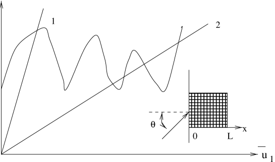
⟨ [ F m ( u ¯ 1 , . . u ¯ n + Δ u ¯ n , . . ) − F m ( u ¯ 1 . . u ¯ n , . . ) ] 2 ⟩ ⟨ ( δ F m ) 2 ⟩ ∼ ( Δ u ¯ n ) 2 . \frac{\langle[F_{m}(\bar{u}_{1},..\bar{u}_{n}+\Delta\bar{u}_{n},..)-F_{m}(\bar{u}_{1}..\bar{u}_{n},..)]^{2}\rangle}{\langle(\delta F_{m})^{2}\rangle}\sim(\Delta\bar{u}_{n})^{2}. (16)
Eq.15 means that the characteristic period
of
random
oscillations of F m subscript 𝐹 𝑚 F_{m} u ¯ n subscript ¯ 𝑢 𝑛 \bar{u}_{n} Δ u ¯ n ∼ 1 similar-to Δ subscript ¯ 𝑢 𝑛 1 \Delta\bar{u}_{n}\sim 1 m 1 3 superscript 𝑚 1 3 m^{\frac{1}{3}}
It is important that Eqs.14 with large enough m > M = γ 3 4 𝑚 𝑀 superscript 𝛾 3 4 m>M=\gamma^{\frac{3}{4}} u ¯ m ∼ m − 2 3 ≪ 1 similar-to subscript ¯ 𝑢 𝑚 superscript 𝑚 2 3 much-less-than 1 \bar{u}_{m}\sim m^{-\frac{2}{3}}\ll 1 u ¯ m < M subscript ¯ 𝑢 𝑚 𝑀 \bar{u}_{m<M} M 𝑀 M γ − 1 2 m 2 3 ≪ 1 much-less-than superscript 𝛾 1 2 superscript 𝑚 2 3 1 \gamma^{-\frac{1}{2}}m^{\frac{2}{3}}\ll 1 γ ∼ 1 similar-to 𝛾 1 \gamma\sim 1 m ≃ 1 similar-to-or-equals 𝑚 1 m\simeq 1 𝒓 − 𝒓 1 𝒓 subscript 𝒓 1 \mathchoice{{\hbox{\boldmath$\displaystyle r$}}}{{\hbox{\boldmath$\textstyle r$}}}{{\hbox{\boldmath$\scriptstyle r$}}}{{\hbox{\boldmath$\scriptscriptstyle r$}}}-\mathchoice{{\hbox{\boldmath$\displaystyle r$}}}{{\hbox{\boldmath$\textstyle r$}}}{{\hbox{\boldmath$\scriptstyle r$}}}{{\hbox{\boldmath$\scriptscriptstyle r$}}}_{1} K 0 ( 𝒓 , 𝒓 1 ) superscript 𝐾 0 𝒓 subscript 𝒓 1 K^{0}(\mathchoice{{\hbox{\boldmath$\displaystyle r$}}}{{\hbox{\boldmath$\textstyle r$}}}{{\hbox{\boldmath$\scriptstyle r$}}}{{\hbox{\boldmath$\scriptscriptstyle r$}}},\mathchoice{{\hbox{\boldmath$\displaystyle r$}}}{{\hbox{\boldmath$\textstyle r$}}}{{\hbox{\boldmath$\scriptstyle r$}}}{{\hbox{\boldmath$\scriptscriptstyle r$}}}_{1}) | 𝒓 − 𝒓 ′ | ∼ L similar-to 𝒓 superscript 𝒓 bold-′ 𝐿 |\mathchoice{{\hbox{\boldmath$\displaystyle r$}}}{{\hbox{\boldmath$\textstyle r$}}}{{\hbox{\boldmath$\scriptstyle r$}}}{{\hbox{\boldmath$\scriptscriptstyle r$}}}-\mathchoice{{\hbox{\boldmath$\displaystyle r^{\prime}$}}}{{\hbox{\boldmath$\textstyle r^{\prime}$}}}{{\hbox{\boldmath$\scriptstyle r^{\prime}$}}}{{\hbox{\boldmath$\scriptscriptstyle r^{\prime}$}}}|\sim L γ ∼ 1 similar-to 𝛾 1 \gamma\sim 1 u ¯ m > 1 = 0 subscript ¯ 𝑢 𝑚 1 0 \bar{u}_{m>1}=0 m = 1 𝑚 1 m=1
γ − 1 2 u ¯ 1 = F 1 ( u ¯ 1 , 0 , 0 , . . ) \gamma^{-\frac{1}{2}}\bar{u}_{1}=F_{1}(\bar{u}_{1},0,0,..) (17)
It is equivalent to substitution in Eq.1
u ~ ( 𝒓 ) → D L u ¯ 1 n 1 ( 𝒓 ) → ~ 𝑢 𝒓 𝐷 𝐿 subscript ¯ 𝑢 1 subscript 𝑛 1 𝒓 \tilde{u}(\mathchoice{{\hbox{\boldmath$\displaystyle r$}}}{{\hbox{\boldmath$\textstyle r$}}}{{\hbox{\boldmath$\scriptstyle r$}}}{{\hbox{\boldmath$\scriptscriptstyle r$}}})\rightarrow\frac{D}{\sqrt{L}}\bar{u}_{1}n_{1}(\mathchoice{{\hbox{\boldmath$\displaystyle r$}}}{{\hbox{\boldmath$\textstyle r$}}}{{\hbox{\boldmath$\scriptstyle r$}}}{{\hbox{\boldmath$\scriptscriptstyle r$}}}) β 𝛽 \beta F 1 ( u ¯ 1 , 0 , 0 . . ) F_{1}(\bar{u}_{1},0,0..) γ − 1 2 u ¯ 1 superscript 𝛾 1 2 subscript ¯ 𝑢 1 \gamma^{-\frac{1}{2}}\bar{u}_{1} γ > 1 𝛾 1 \gamma>1 u ( 𝒓 ) 𝑢 𝒓 u(\mathchoice{{\hbox{\boldmath$\displaystyle r$}}}{{\hbox{\boldmath$\textstyle r$}}}{{\hbox{\boldmath$\scriptstyle r$}}}{{\hbox{\boldmath$\scriptscriptstyle r$}}}) ( τ f τ D ) 2 K ( 𝒓 , 𝒓 ′ ) superscript 𝜏 𝑓 subscript 𝜏 𝐷 2 𝐾 𝒓 superscript 𝒓 ′ (\frac{\tau{f}}{\tau_{D}})^{2}K(\mathchoice{{\hbox{\boldmath$\displaystyle r$}}}{{\hbox{\boldmath$\textstyle r$}}}{{\hbox{\boldmath$\scriptstyle r$}}}{{\hbox{\boldmath$\scriptscriptstyle r$}}},\mathchoice{{\hbox{\boldmath$\displaystyle r$}}}{{\hbox{\boldmath$\textstyle r$}}}{{\hbox{\boldmath$\scriptstyle r$}}}{{\hbox{\boldmath$\scriptscriptstyle r$}}}^{\prime}) u ( 𝒓 ) 𝑢 𝒓 u(\mathchoice{{\hbox{\boldmath$\displaystyle r$}}}{{\hbox{\boldmath$\textstyle r$}}}{{\hbox{\boldmath$\scriptstyle r$}}}{{\hbox{\boldmath$\scriptscriptstyle r$}}}) F 1 ( u ¯ 1 , 0 , 0 . . ) F_{1}(\bar{u}_{1},0,0..) γ − 1 2 u ¯ 1 superscript 𝛾 1 2 subscript ¯ 𝑢 1 \gamma^{-\frac{1}{2}}\bar{u}_{1} γ > 1 𝛾 1 \gamma>1 ⟨ ( β L 3 d d ϵ ∫ n ( 𝒓 ) 𝑑 𝒓 ) 2 ⟩ > 1 delimited-⟨⟩ superscript 𝛽 superscript 𝐿 3 𝑑 𝑑 italic-ϵ 𝑛 𝒓 differential-d 𝒓 2 1 \langle(\frac{\beta}{L^{3}}\frac{d}{d\epsilon}\int n(\mathchoice{{\hbox{\boldmath$\displaystyle r$}}}{{\hbox{\boldmath$\textstyle r$}}}{{\hbox{\boldmath$\scriptstyle r$}}}{{\hbox{\boldmath$\scriptscriptstyle r$}}})d\mathchoice{{\hbox{\boldmath$\displaystyle r$}}}{{\hbox{\boldmath$\textstyle r$}}}{{\hbox{\boldmath$\scriptstyle r$}}}{{\hbox{\boldmath$\scriptscriptstyle r$}}})^{2}\rangle>1 [13]
We would like to mention that even at γ < 1 𝛾 1 \gamma<1 u ( 𝒓 ) 𝑢 𝒓 u(\mathchoice{{\hbox{\boldmath$\displaystyle r$}}}{{\hbox{\boldmath$\textstyle r$}}}{{\hbox{\boldmath$\scriptstyle r$}}}{{\hbox{\boldmath$\scriptscriptstyle r$}}}) γ 𝛾 \gamma
At γ ≫ 1 much-greater-than 𝛾 1 \gamma\gg 1 γ 1 2 superscript 𝛾 1 2 \gamma^{\frac{1}{2}} γ ≫ 1 much-greater-than 𝛾 1 \gamma\gg 1 u ¯ 1 subscript ¯ 𝑢 1 \bar{u}_{1} 1 < m < M 1 𝑚 𝑀 1<m<M | u ¯ m | < γ 1 2 m − 2 3 subscript ¯ 𝑢 𝑚 superscript 𝛾 1 2 superscript 𝑚 2 3 |\bar{u}_{m}|<\gamma^{\frac{1}{2}}m^{-\frac{2}{3}} m − t h 𝑚 𝑡 ℎ m-th F m ( u ¯ 1 … ) subscript 𝐹 𝑚 subscript ¯ 𝑢 1 … F_{m}(\bar{u}_{1}...) N of Eqs.14,1 is
proportional to the volume of the
manifold | u ¯ m | < γ 1 2 m − 2 3 subscript ¯ 𝑢 𝑚 superscript 𝛾 1 2 superscript 𝑚 2 3 |\bar{u}_{m}|<\gamma^{\frac{1}{2}}m^{-\frac{2}{3}} m < M 𝑚 𝑀 m<M
N ∼ γ M 2 ∏ 1 M m − 2 3 = exp ( a γ 3 4 ) similar-to 𝑁 superscript 𝛾 𝑀 2 superscript subscript product 1 𝑀 superscript 𝑚 2 3 𝑎 superscript 𝛾 3 4 N\sim\gamma^{\frac{M}{2}}\prod_{1}^{M}m^{-\frac{2}{3}}=\exp(a\gamma^{\frac{3}{4}}) (18)
where a ∼ 1 similar-to 𝑎 1 a\sim 1
Similar phenomenon may occur in
disordered metals with interacting
electrons. The system can be unstable with respect to creation of random
magnetic
moments. In this case n ( 𝒓 ) 𝑛 𝒓 n(\mathchoice{{\hbox{\boldmath$\displaystyle r$}}}{{\hbox{\boldmath$\textstyle r$}}}{{\hbox{\boldmath$\scriptstyle r$}}}{{\hbox{\boldmath$\scriptscriptstyle r$}}}) [12] n ( 𝒓 ) 𝑛 𝒓 n(\mathchoice{{\hbox{\boldmath$\displaystyle r$}}}{{\hbox{\boldmath$\textstyle r$}}}{{\hbox{\boldmath$\scriptstyle r$}}}{{\hbox{\boldmath$\scriptscriptstyle r$}}}) n ( 𝒓 ) 𝑛 𝒓 n(\mathchoice{{\hbox{\boldmath$\displaystyle r$}}}{{\hbox{\boldmath$\textstyle r$}}}{{\hbox{\boldmath$\scriptstyle r$}}}{{\hbox{\boldmath$\scriptscriptstyle r$}}}) 𝒓 𝒓 \textstyle r
Above we considered the case when
ϕ ( 𝒓 , t ) = ϕ ( 𝒓 , ϵ ) exp ( i ϵ t ) italic-ϕ 𝒓 𝑡 italic-ϕ 𝒓 italic-ϵ 𝑖 italic-ϵ 𝑡 \phi(\mathchoice{{\hbox{\boldmath$\displaystyle r$}}}{{\hbox{\boldmath$\textstyle r$}}}{{\hbox{\boldmath$\scriptstyle r$}}}{{\hbox{\boldmath$\scriptscriptstyle r$}}},t)=\phi(\mathchoice{{\hbox{\boldmath$\displaystyle r$}}}{{\hbox{\boldmath$\textstyle r$}}}{{\hbox{\boldmath$\scriptstyle r$}}}{{\hbox{\boldmath$\scriptscriptstyle r$}}},\epsilon)\exp(i\epsilon t) n ( 𝒓 ) = | ϕ ( 𝒓 , t ) | 2 𝑛 𝒓 superscript italic-ϕ 𝒓 𝑡 2 n(\mathchoice{{\hbox{\boldmath$\displaystyle r$}}}{{\hbox{\boldmath$\textstyle r$}}}{{\hbox{\boldmath$\scriptstyle r$}}}{{\hbox{\boldmath$\scriptscriptstyle r$}}})=|\phi(\mathchoice{{\hbox{\boldmath$\displaystyle r$}}}{{\hbox{\boldmath$\textstyle r$}}}{{\hbox{\boldmath$\scriptstyle r$}}}{{\hbox{\boldmath$\scriptscriptstyle r$}}},t)|^{2} exp ( 3 i ϵ t ) 3 𝑖 italic-ϵ 𝑡 \exp(3i\epsilon t) ϕ ( 𝒓 ) italic-ϕ 𝒓 \phi(\mathchoice{{\hbox{\boldmath$\displaystyle r$}}}{{\hbox{\boldmath$\textstyle r$}}}{{\hbox{\boldmath$\scriptstyle r$}}}{{\hbox{\boldmath$\scriptscriptstyle r$}}}) k l 2 γ L ≪ 1 much-less-than 𝑘 superscript 𝑙 2 𝛾 𝐿 1 \frac{kl^{2}\gamma}{L}\ll 1 γ ≫ 1 much-greater-than 𝛾 1 \gamma\gg 1
Finally, we would like to mention that the problem considered above
is similar
to the problem of classical chaos, where the the sensitivity of
trajectories of motion to changes in boundary conditions exponentially
increases with the sample size (See for example [14]
Work of B.S. was supported by Division of Material Sciences, U.S.National
Science Foundation under Contract No.DMR-9625370. Work of A.Z. was
supported by Russian Fund of Fundamental Investigations under grant
97-02-18078.
REFERENCES
[1]
P.A.Lee, A.D.Stone, Phys.Rev.Lett.55, 1622, 1985.
[2]
B.Altshuler, B.Spivak, JETP Lett.42, 447, 1986.
[3]
S.Feng, P.Lee, A.D.Stone, Phys.Rev.Lett.56,1560,1986.
[4]
B.Spivak, A.Zyuzin, ”Mesoscopic Fluctuations of Current Density
in Disordered Conductors” In ”Mesoscopic Phenomena in Solids” Ed.
B.Altshuler, P.Lee, R.Webb, Modern Problems in Condensed Matter Sciences
vol.30, 1991.
[5]
B.Simons, B.Altshuler, Phys.Rev.Lett.70, 4063,1993.
[6]
L.Landau, E.Lifshitz, ”Electrodynamics of continuous media”, 1968.
[7]
V.E.Zakharov, V.S.Lvov, G.Falkovich, ”Kolmogorov spectra of
turbulence” Springer-Verlag, 1992.
[8]
B.B.Kadomzev, ”Collective phenomena in plasma”, Nauka, Moskow,
1976.
[9]
A.Abrikosov, L.Gorkov, I.Dzyialoshinski, ”Methods of quantum
field theory in statistical physics” NY,1963.
[10]
In the case β > 0 𝛽 0 \beta>0 l 𝑙 l [6]
[11]
A.Zyuzin, B.Spivak, Sov.Phys.JETP.66,560,1987.
[12]
A.M.Finkelshtein, Sov.Sci.Rev.A, Phys. 14, 1, 1990.
[13]
A.A.Abrikosov ”Fundamentals of the theory of metals”, North
Holland, 1988.
[14]
A.J. Lichtenberg, M.A Lieberman, ”Regular and stochastic motion”,
New York, Springer-Verlag, 1992.
FIG. 1.: Graphical solution of Eq.16. The wavy line corresponds to
F 1 ( u ¯ 1 ) subscript 𝐹 1 subscript ¯ 𝑢 1 F_{1}(\bar{u}_{1}) γ − 1 2 u ¯ 1 superscript 𝛾 1 2 subscript ¯ 𝑢 1 \gamma^{-\frac{1}{2}}\bar{u}_{1} γ ∼ 1 similar-to 𝛾 1 \gamma\sim 1 γ ≫ 1 much-greater-than 𝛾 1 \gamma\gg 1
FIG. 2.: Solid lines correspond to Green functions of Eq.1 with
β = 0 𝛽 0 \beta=0 π l m 2 δ ( 𝒓 − 𝒓 1 ) 𝜋 𝑙 superscript 𝑚 2 𝛿 𝒓 subscript 𝒓 1 \frac{\pi}{lm^{2}}\delta(\mathchoice{{\hbox{\boldmath$\displaystyle r$}}}{{\hbox{\boldmath$\textstyle r$}}}{{\hbox{\boldmath$\scriptstyle r$}}}{{\hbox{\boldmath$\scriptscriptstyle r$}}}-\mathchoice{{\hbox{\boldmath$\displaystyle r$}}}{{\hbox{\boldmath$\textstyle r$}}}{{\hbox{\boldmath$\scriptstyle r$}}}{{\hbox{\boldmath$\scriptscriptstyle r$}}}_{1}) β 𝛽 \beta Δ u ( 𝒓 ) Δ 𝑢 𝒓 \Delta u(\mathchoice{{\hbox{\boldmath$\displaystyle r$}}}{{\hbox{\boldmath$\textstyle r$}}}{{\hbox{\boldmath$\scriptstyle r$}}}{{\hbox{\boldmath$\scriptscriptstyle r$}}})