Integrability of the critical point of the Kagomé three-state Potts model

Abstract

The vicinity of the critical point of the three-state Potts model on a Kagomé lattice is studied by mean of Random Matrix Theory. Strong evidence that the critical point is integrable is given.

I Introduction

The $q$-state Potts model [1], being one of the simplest generalization of the Ising model, is a challenging model of classical lattice statistical mechanics. Despite its apparent simplicity it has not yet been analytically solved for a number of states $q>2$ even in two dimensions (for a review see [2]). The square, the triangular and the hexagonal lattice have been shown to be integrable at the critical point. The free energy the correlation function have been calculated. Out of the critical point the free energy has not been calculated, moreover strong indications that the model is not integrable have been given [3]. On another hand the two dimensional Kagomé lattice is of great interest both from the statistical point of view and from solid state point of view. The anti ferromagnetic Kagomé lattice provides an example of geometrically frustrated spin system [4]. Several experiments on the so-called SCGO compounds family suggest the existence of a ”spin-liquid” phase transition [5]. It has also been seen as topological spin glass [6].

The critical point of the Potts model on the Kagomé lattice is known in the Ising ($q=2$) case only. However, an algebraic variety has been conjectured to be critical for the checkerboard square lattice with multi spin interaction in  [7]. From this conjecture the critical point of the Potts Kagomé lattice has been deduced [7]. This value has recently been confirmed with high precision by extensive Monte-Carlo simulation [8], so that the actual critical point is at least extremely closed from the conjectured point. The aim of this letter is not give another numerical confirmation of this conjecture, but to address the question of a possible integrability of the critical point. Indeed it is possible that the critical point of the Kagomé $q=3$ Potts model is of the same nature as the critical point of the square, hexagonal or triangular lattice, ie an integrable point. It is however also possible that this point is not integrable, as is, for example, the the critical point of the three dimensional Ising cubic lattice [3]. This letter is intended to give an answer to this question. It is organized as follows: in a first paragraph we sketch briefly the basics of Random Matrix Theory (RMT) applied to classical lattice statistical mechanics, and recall how it acts as an ‘integrability detector’. In the next paragraph we give a more convenient formulation of the Kagomé lattice as a checkerboard Interaction-Round-a-Face (IRF) model, and we discuss the symmetries of the corresponding transfer matrix. In the final paragraph the results are presented and discussed.

II The RMT methodology

The RMT lattice statistical mechanics has first been introduced for Quantum one dimensional system [9, 10], it has then been extended to classical two dimensional lattices [11]. Roughly speaking the main idea is to compare the given Hamiltonian to an ‘average Hamiltonian’. Among all Hamiltonians, integrable Hamiltonians are extremely peculiar and show significant difference with ‘average Hamiltonian’. To be more specific one is interested in the statistical properties of the discrete spectrum viewed as an infinite set of real numbers. One compares the statistical properties of the spectrum of the system under consideration with the one of random matrices from a suitable statistical ensemble. For an integrable system it is found that the spectrum as many properties of a set of independent numbers, ie the suitable matrix statistical ensemble is the set of the diagonal matrices with independent normal centered entries. By contrast, for a non-integrable time reversal symmetric system the spectrum is well described by spectrum of matrices from the so-called Gaussian Orthogonal Ensemble (GOE) of symmetric matrices with independent normal centered entries. The eigenvalue spacing distribution $P(s)$ discriminates well between these two limiting cases: $P(s)\,ds$ is the probability that the difference between two consecutive eigenvalues belongs to the interval $[s,s+ds]$. It is simple to show that for independent eigenvalues one has $P(s)=e^{-s}$. For GOE matrices $P(s)$ is extremely close (actually strictly equal for $2\times 2$ matrices) to the Wigner surmise $W(s)={\pi\over 2}s\exp(-\pi s^{2}/4)$. Provided that the proper normalization explained below has been performed, and if the system size is large enough, then the distribution $P(s)$ of the system under consideration is close to one of the exponential or Wigner distribution. To quantify this “proximity” one introduces the parametrized distribution

$$P_{\beta}(s)=c(1+\beta)s^{\beta}\exp\left(-cs^{\beta+1}\right)\;,$$ (1)

with $c=\left[\Gamma\left({\beta+2\over\beta+1}\right)\right]^{1+\beta}$, which is one of the infinitely many possible interpolations between the exponential and Wigner distribution. For $\beta=0$ one recovers the exponential law and for $\beta=1$ one recovers the Wigner law. The full lines on Fig. 2 represents these two distributions. Parameter $\beta$ is interpreted as the repulsion between eigenvalues. $P(s)$ is a quantity involving only pairs of eigenvalues; a quantity involving more than two eigenvalues is the spectral rigidity

$$\Delta_{3}(\lambda)=\left\langle{1\over\lambda}\min_{a,b}\int_{\alpha-l/2}^{\alpha+\lambda/2}(N_{u}(\epsilon)-a\epsilon-b)^{2}d\epsilon\right\rangle_{\alpha}\;,$$ (2)

where $N_{u}(\epsilon)\equiv\sum_{i}\Theta(\epsilon-\epsilon_{i})$ is the integrated density of unfolded eigenvalues and $\langle\dots\rangle_{\alpha}$ denotes an average over $\alpha$. It provides a finer test of the closeness of a spectrum with a GOE spectrum or with independent numbers. These two limiting cases are shown of Fig. 3 as full lines. For the classical lattice system, like spin models or vertex models, the transfer matrix [13] is considered instead of the Hamiltonian which generally has a trivial spectrum.

The operational procedure has been explained in details in [12, 13]. It consists in two main steps. One first sort the states according to their symmetries: states of different symmetries have to be considered separately. Then, since universal properties cannot be found on the row spectrum, a procedure of “normalization”, known as the unfolding, is performed: it consists in imposing a local density of eigenvalues of the order of unity. Then the statistical properties of the sorted and unfolded spectrum are analyzed. Note that this analysis requires real eigenvalues. This is generally insured by the of the Hamiltonian.

III Transfer matrix of the Potts model on the Kagomé lattice

The Kagomé lattice is a two dimensional lattice depicted on Figure 1. The black circles represent the sites, and the lines are the coupling bonds. The partition function reads

$$Z_{\rm kag}=\prod_{<i,j>}{K_{i\,j}^{\delta(\sigma_{i},\sigma_{j})}}$$ (3)

$<i,j>$ denotes the neighboring sites on the Kagomé lattice, $\delta$ is the Kronecker symbol, $K_{i\,j}=K_{1},K_{2}$ or $K_{3}$ for each of the three types of bonds, and $\sigma_{i}$ can take one of the three values 0, 1, 2. The Kagomé lattice can be regarded as a lattice of basic “cells” (1,2,3,4) as shown on Fig. 1. Each cell consists in a up pointing triangle sharing a site (site labelled 0 on the figure) with a down pointing triangle. These cells are disposed on every other (say black) plaquettes of checkerboard. To see the correspondence with an IRF model on a checkerboard lattice, one perform a partial summation on the central site (site 0), seeking coupling constants such that

$$W_{\rm IRF}(\sigma_{1},\sigma_{2},\sigma_{3},\sigma_{4})=\sum_{\sigma_{0}}W_{\rm kag}(\sigma_{1},\sigma_{2},\sigma_{3},\sigma_{4};\sigma_{0})$$ (4)

This is possible if one introduces multi spin interaction. The general correspondence is given in Appendix A. For the isotropic $K_{1}=K_{2}=K_{3}=K$ case the Boltzmann weights of the plaquettes are given by

$$W_{\rm kag}(\sigma_{1},\sigma_{2},\sigma_{3},\sigma_{4};\sigma_{0})=K^{\delta_{0,1}+\delta_{0,2}+\delta_{0,3}+\delta_{0,4}+\delta_{1,2}+\delta_{3,4}}$$ (5)

and

$$W_{\rm IRF}(\sigma_{1},\sigma_{2},\sigma_{3},\sigma_{4})=L_{h}^{\delta_{1,2}+\delta_{3,4}}\,L_{v}^{\delta_{1,3}+\delta_{2,4}}\,L_{d}^{\delta_{1,4}+\delta_{2,3}}\,T^{\delta_{1,2,3}+\delta_{1,2,4}+\delta_{1,3,4}+\delta_{2,3,4}}\,F^{\delta_{1,2,3,4}}$$ (6)

where $\delta_{i,j}=\delta(\sigma_{i},\sigma_{j})$ and $\delta_{i,j,k}=\delta(\sigma_{i},\sigma_{j},\sigma_{k})$ ($\sigma_{i}=1,2,3,4$). The parameters of the IRF model are given as a function of the parameters of the Kagomé by:

$$L_{h} = KL_{v}=KL_{d}=\frac{2K^{2}+1}{K+2}$$ (7)

$$T = \frac{(K+2)(K^{3}+K+1)K}{(2K^{2}+1)^{2}}$$ (8)

$$F = \frac{(K^{4}+2)(2K^{2}+K+1)^{3}}{(K^{3}+K+1)^{4}}$$ (9)

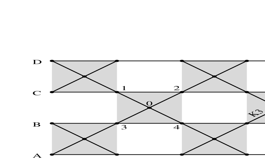
FIG. 1.: Correspondence between the Kagomé lattice and the checkerboard IRF model.

From a computational point of view it is more convenient to use the IRF representation, this is the form chosen in the calculations presented here. A first difficulty in constructing the transfer matrix comes from the fact the actual transfer matrix which brings from row A to row C on Fig. 1 is the product of the two transfer matrices bringing respectively from row A to row B and from row B to row C. As a result the calculation of a single entry of the transfer matrix involves a combination of sums and products over $N$ terms, $N=3^{L}$ being the size of the matrix ($L$ is the linear size of the rows, $L=6$ on Fig. 1). This greatly slows down the calculations. Another difficulty comes with the fact that, unlike simpler lattice, there is no way to make symmetric the transfer matrix $T$, so that the eigenvalues are complex. It is still possible to deal with complex eigenvalues. In this case integrability also leads to independent eigenvalues, and non integrability leads to repulsion. However, in practice, it is much more difficult to make the distinction, since in two dimensions repulsion is less effective. Therefore we have chosen to analyze the statistical properties of the operator ${\cal T}=(T+\tilde{T})/2$.

In the actual computation, the transfer matrix calculated is the diagonal-to-diagonal transfer matrix. As explained in the previous paragraph one needs to find the symmetries of the operator ${\cal T}$. Let us define the translation operator $t$, the reflection $r$, and the color operator $c$

$$t\;|\sigma_{0},\sigma_{1},\cdots,\sigma_{L-1}> = |\sigma_{1},\sigma_{2},\cdots\sigma_{0}>$$ (10)

$$r\;|\sigma_{0},\sigma_{1},\cdots,\sigma_{L-1}> = |\sigma_{L-1},\sigma_{L-2},\cdots,\sigma_{0}>$$ (11)

$$c\;|\sigma_{0},\sigma_{1},\cdots,\sigma_{L-1}> = |\sigma_{0}+1,\sigma_{1}+1,\cdots,\sigma_{L-1}+1>$$ (12)

where the sum are taken modulo 3. It is easy to see the three operators $t$, $r$ and $c$ commute with ${\cal T}$, and that $c$ commutes with both $t$ and $r$. Thus the symmetry group is the direct product ${\cal D}_{L}\otimes{\cal D}_{3}$ where ${\cal D}_{L}$ is the dihedral group of index $L$. The irreducible representations of this group are simply the matrix product of elements of ${\cal D}_{L}$ and ${\cal D}_{3}$ (see details in [14]). The sizes of the blocks corresponding to the different representations are given in Tab. I. In the statistical analysis the blocks of size smaller than 100 have been discarded to minimize small size effects.

IV Results and Conclusion

Using the IRF representation of the Kagomé lattice we have calculated for different values of the exponential of the coupling constant $K$ the symmetrized diagonal-to-diagonal transfer matrix ${\cal T}(K)$ for $L=8$. The size of the matrix ${\cal T}$ is $3^{8}=6561$. For sizes smaller than $L=8$, the blocks are quite small, giving poor statistics. On another hand the size $L=9$ is out of reach of your computing possibility, especially due to the facts that ${\cal T}$ is a matrix product with all entries non zero (in contrast with most quantum Hamiltonian) as explained in the previous paragraph. So we stick to the case $L=8$ and perform the analysis for different values of $K$. The matrix is projected in the different invariant subspaces, yielding matrix blocks of smaller sizes (see Tab. I). Within blocks there is no degeneracy left, proving that the symmetry group used is the largest symmetry group for this model, as it should. The spectrum of the 13 larger blocks is then unfolded, leading to 2187 eigenvalues distributed in 13 sub-sets. The eigenvalues spacing distribution $P(s)$ as well as the rigidity $\Delta_{3}$ are calculated. We present on Fig. 2 and Fig. 3 the results for two values of $K$. Firstly for $K=K_{c}$ where $K_{c}$ is the value predicted by the Wu’s conjecture, which is known to be at least extremely close the the actual critical value. And secondly for $K=2$ which is sufficiently far from the critical value, and neither too small nor too big: extremal values leads to accuracy problems. The results are unambiguous: close to the transition point the distribution of eigenvalues is very close to an exponential, whereas out of this point it is close to a Wigner distribution. This is clearly seen on Fig. 2 where the numerical data are presented for both cases together with the exponential law and the Wigner distribution. The best fit values of $\beta$ (see Eq. 1) are $\beta(K_{c})=0.01$ and $\beta(2)=1.02$. This is a strong indication that the critical point is integrable. To further support this result, the rigidity Eq. 2 has also been calculated for the same value of $K$. The results are shown on Fig. 3, where the numerical data and the two limiting cases of a GOE spectrum and of independent numbers are presented. The agreement between the expected behavior and the observed behavior is very good, at least up to an “energy scale” of the order of 15, (ie 15 eigenvalues since the mean density of eigenvalues is one). The number variance $\Sigma^{2}(l)=\left\langle\left[N_{u}(\epsilon+l/2)-N_{u}(\epsilon-l/2)-l\right]^{2}\right\rangle_{\epsilon}$ where the brackets denote an averaging over $\epsilon$ has also been calculated, giving results not presented here, in perfect agreement with the results for the spectral rigidity $\Delta_{3}$.

In conclusion a RMT analysis performed on the symmetrized transfer matrix of the Kagomé lattice seen as an IRF checkerboard model shows that the critical point, very close or equal to the Wu’s conjecture, is an integrable point. This is in agreement the conformal theories of the two dimensional lattice statistical mechanics. The only example of a critical point where the transfer matrix eigenvalues spacing distribution is of Wigner type is the 3-dimensional Ising case.

0	1	2	3	4	5	6	7	8	9	10	11	12	13	14	15	16	17	18	19	20
1	1	2	1	1	2	1	1	2	1	1	2	2	2	4	2	2	4	2	2	4
100	66	166	46	66	112	72	53	125	72	80	152	130	140	270	142	134	276	130	140	270

TABLE I.: Sizes and degeneracies of the different blocks for $L=8$. The first row is the label of the representation, the second is the dimension of the representation (ie degeneracy of the corresponding eigenvalues) and the third row is the size of the block to be diagonalized.

FIG. 2.: Distribution of eigenvalue spacings for $K\simeq K_{c}$. The linear size of the lattice is $L=8$, leading to Hilbert space of size 6561. 1910 eigenvalues are included in the statistic. The diamonds corresponds to the critical point $K=K_{c}$, and the square corresponds to the the value $K=2$.

FIG. 3.: Rigidity $\Delta_{3}$ as a function of $\lambda$ for the same data as in Fig. 2.

A Kagomé lattice and checkerboard IRF model

For a non-isotropic Kagomé lattice the Boltzmann weight of a basic cell (see Fig 1) is

$$W_{\rm kag}(\sigma_{1},\sigma_{2},\sigma_{3},\sigma_{4};\sigma_{0})=K_{1}^{\delta_{1,2}+\delta_{3,4}}K_{2}^{\delta_{0,1}+\delta_{0,4}}K_{3}^{\delta_{0,2}+\delta_{0,3}}$$ (A1)

and for IRF checkerboard it is

$$W_{\rm IRF}(\sigma_{1},\sigma_{2},\sigma_{3},\sigma_{4})=L_{12}^{\delta_{1,2}}L_{34}^{\delta_{3,4}}L_{13}^{\delta_{1,3}}L_{24}^{\delta_{2,4}}L_{14}^{\delta_{1,4}}L_{23}^{\delta_{2,3}}L_{123}^{\delta_{1,2,3}}L_{124}^{\delta_{1,2,4}}L_{134}^{\delta_{1,3,4}}L_{234}^{\delta_{2,3,4}}L_{1234}^{\delta_{1,2,3,4}}\left(L_{12}^{34}\right)^{\delta_{12}\delta_{34}}\left(L_{13}^{24}\right)^{\delta_{13}\delta_{24}}$$ (A2)

The notation are the same as in the text Eq. 6. The parameters of the IRF model are given as a function of the parameters of the Kagomé by:

$$L_{12}(K_{1},K_{2},K_{3}) = L_{34}(K_{1},K_{2},K_{3})=K_{1}L_{13}(K_{2},K_{3})=K_{1}L_{24}(K_{2},K_{3})$$ (A3)

$$= K_{1}\frac{(K_{2}K_{3}+K_{2}+K_{3})(1+K_{2}^{2}+K_{3}^{2})}{2K_{2}^{3}+K_{2}^{2}K_{3}^{2}+4K_{2}K_{3}+2K_{3}^{3}}$$ (A4)

$$L_{14}(K_{2},K_{3}) = L_{23}(K_{3},K_{2})$$ (A5)

$$= \frac{K_{2}^{2}+K_{3}^{2}+1}{2K_{2}+2K_{3}^{2}}$$ (A6)

$$L_{234}(K_{2},K_{3}) = L_{134}(K_{3},K_{2})=L_{124}(K_{3},K_{2})=L_{123}(K_{2},K_{3})$$ (A7)

$$= \frac{(K_{3}^{2}+2K_{2})(K_{2}K_{3}^{2}+K_{2}+1)(K_{2}^{2}+2K_{3})^{2}}{((K_{2}K_{3}+K_{2}+K_{3})(K_{2}^{2}+K_{3}^{2}+1))^{2}}$$ (A8)

$$L_{12}^{34}(K_{2},K_{3}) = L_{13}^{24}(K_{2},K_{3})$$ (A9)

$$= \frac{(2K_{2}K_{3}+1)(2K_{2}^{3}+K_{2}^{2}K_{3}^{2}+4K_{2}K_{3}+2K_{3}^{3})}{(K_{2}^{2}+K_{3}^{2}+1)(K_{2}K_{3}+K_{2}+K_{3})^{2}}$$ (A10)

$$L_{1234}(K2,K3) = \frac{(K_{2}^{2}K_{3}^{2}+2)(K_{2}^{2}+K_{3}^{2}+1)^{4}}{((K_{2}+2K_{3})(K_{3}+2K_{2}))^{2}}$$ (A12)

$$\times\frac{(K_{2}K_{3}+K_{3}+K_{2})^{4}}{((K_{2}^{2}K_{3}+K_{3}+1)(K_{2}K_{3}^{2}+K_{2}+1))^{2}}$$

REFERENCES

-
[1]
R.B. Potts
Proc. Camb. Phil. Soc. 48,106 (1952) -
[2]
F.Y. Wu
Rev. Mod. Phy. 54,235 (1982) -
[3]
H. Meyer.
Ph.D. dissertation, Grenoble (1996). -
[4]
Y.J. Uemera et al.
Phys. Rev. Lett.73, 3306 (1994). -
[5]
P. Schiffer and I. Daruka,
Phys. Rev. b56, 13712 (1997). -
[6]
P. Chandra, P. Coleman and I. Ritchey
J. Phys. I France 3 591 (1991). -
[7]
F.Y. Wu.
J. Phys. C12, L645 (1979). -
[8]
J.A. Chen, C.K. Hu and F.Y. Wu.
J. Phys. A, (1998). -
[9]
G. Montambaux, D. Poilblanc, J Bellissard and C. Sire.
Phys. Rev. Lett. 70 497, (1993). -
[10]
T. Hsu, J.C. Anglès d’Auriac.
Phys. Rev. B47 21 14291 (1993). -
[11]
H. Meyer and J. C. Anglès d’Auriac.
J. Phys. A: Math. Gen. 29 L483 (1996). -
[12]
H. Meyer, J. C. Anglès d’Auriac and J.M. Maillard.
Phys. Rev. E55, 5380 (1997). -
[13]
H. Meyer, J. C. Anglès d’Auriac and H. Bruus
Phys. Rev. E55, 6608 (1997). -
[14]
H. Bruus and J. C. Anglès d’Auriac.
Phys. Rev. B55, 9142 (1997).